55.2 Graphical analysis of discrete dynamical systems

Function: chaosgame ([[x1, y1]…[xm, ym]], [x0, y0], b, n, options, …); ¶

Implements the so-called chaos game: the initial point (x0, y0) is plotted and then one of the m points [x1, y1]…xm, ym] will be selected at random. The next point plotted will be on the segment from the previous point plotted to the point chosen randomly, at a distance from the random point which will be b times that segment’s length. The procedure is repeated n times. The options are the same as for plot2d.

Example. A plot of Sierpinsky’s triangle:

(%i1) chaosgame([[0, 0], [1, 0], [0.5, sqrt(3)/2]], [0.1, 0.1], 1/2,
                 30000, [style, dots]);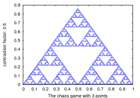

Categories: Package dynamics · Plotting ·

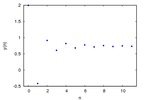
Function: evolution (F, y0, n, …, options, …); ¶

Draws n+1 points in a two-dimensional graph, where the horizontal coordinates of the points are the integers 0, 1, 2, ..., n, and the vertical coordinates are the corresponding values y(n) of the sequence defined by the recurrence relation

        y(n+1) = F(y(n))

With initial value y(0) equal to y0. F must be an expression that depends only on one variable (in the example, it depend on y, but any other variable can be used), y0 must be a real number and n must be a positive integer. This function accepts the same options as plot2d.

Example.

(%i1) evolution(cos(y), 2, 11);

Categories: Package dynamics · Plotting ·

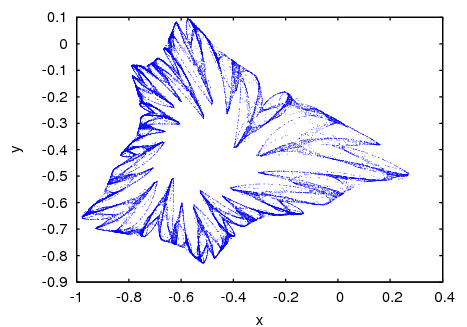
Function: evolution2d ([F, G], [u, v], [u0, y0], n, options, …); ¶

Shows, in a two-dimensional plot, the first n+1 points in the sequence of points defined by the two-dimensional discrete dynamical system with recurrence relations

        u(n+1) = F(u(n), v(n))    v(n+1) = G(u(n), v(n))

With initial values u0 and v0. F and G must be two expressions that depend only on two variables, u and v, which must be named explicitly in a list. The options are the same as for plot2d.

Example. Evolution of a two-dimensional discrete dynamical system:

(%i1) f: 0.6*x*(1+2*x)+0.8*y*(x-1)-y^2-0.9$
(%i2) g: 0.1*x*(1-6*x+4*y)+0.1*y*(1+9*y)-0.4$
(%i3) evolution2d([f,g], [x,y], [-0.5,0], 50000, [style,dots]);

And an enlargement of a small region in that fractal:

(%i9) evolution2d([f,g], [x,y], [-0.5,0], 300000, [x,-0.8,-0.6],
                  [y,-0.4,-0.2], [style, dots]);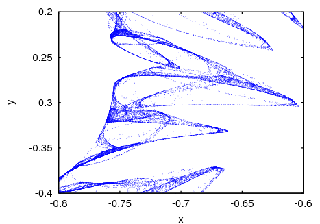

Categories: Package dynamics · Plotting ·

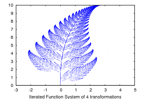
Function: ifs ([r1, …, rm], [A1,…, Am], [[x1, y1], …, [xm, ym]], [x0, y0], n, options, …); ¶

Implements the Iterated Function System method. This method is similar to the method described in the function chaosgame. but instead of shrinking the segment from the current point to the randomly chosen point, the 2 components of that segment will be multiplied by the 2 by 2 matrix Ai that corresponds to the point chosen randomly.

The random choice of one of the m attractive points can be made with a non-uniform probability distribution defined by the weights r1,...,rm. Those weights are given in cumulative form; for instance if there are 3 points with probabilities 0.2, 0.5 and 0.3, the weights r1, r2 and r3 could be 2, 7 and 10. The options are the same as for plot2d.

Example. Barnsley’s fern, obtained with 4 matrices and 4 points:

(%i1) a1: matrix([0.85,0.04],[-0.04,0.85])$
(%i2) a2: matrix([0.2,-0.26],[0.23,0.22])$
(%i3) a3: matrix([-0.15,0.28],[0.26,0.24])$
(%i4) a4: matrix([0,0],[0,0.16])$
(%i5) p1: [0,1.6]$
(%i6) p2: [0,1.6]$
(%i7) p3: [0,0.44]$
(%i8) p4: [0,0]$
(%i9) w: [85,92,99,100]$
(%i10) ifs(w, [a1,a2,a3,a4], [p1,p2,p3,p4], [5,0], 50000, [style,dots]);

Categories: Package dynamics · Plotting ·

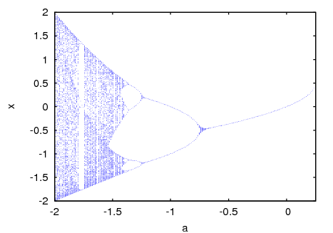
Function: orbits (F, y0, n1, n2, [x, x0, xf, xstep], options, …); ¶

Draws the orbits diagram for a family of one-dimensional discrete dynamical systems, with one parameter x; that kind of diagram is used to study the bifurcations of an one-dimensional discrete system.

The function F(y) defines a sequence with a starting value of y0, as in the case of the function evolution, but in this case that function will also depend on a parameter x that will take values in the interval from x0 to xf with increments of xstep. Each value used for the parameter x is shown on the horizontal axis. The vertical axis will show the n2 values of the sequence y(n1+1),..., y(n1+n2+1) obtained after letting the sequence evolve n1 iterations. In addition to the options accepted by plot2d, it accepts an option pixels that sets up the maximum number of different points that will be represented in the vertical direction.

Example. Orbits diagram of the quadratic map, with a parameter a:

(%i1) orbits(x^2+a, 0, 50, 200, [a, -2, 0.25], [style, dots]);

To enlarge the region around the lower bifurcation near x = -1.25 use:

(%i2) orbits(x^2+a, 0, 100, 400, [a,-1,-1.53], [x,-1.6,-0.8],
             [nticks, 400], [style,dots]);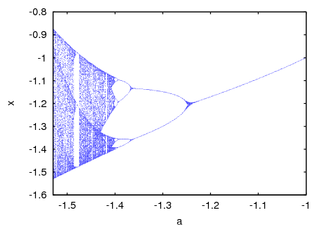

Categories: Package dynamics · Plotting ·

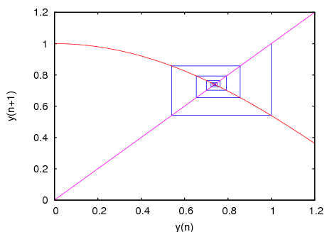
Function: staircase (F, y0, n,options,…); ¶

Draws a staircase diagram for the sequence defined by the recurrence relation

        y(n+1) = F(y(n))

The interpretation and allowed values of the input parameters is the same as for the function evolution. A staircase diagram consists of a plot of the function F(y), together with the line G(y) = y. A vertical segment is drawn from the point (y0, y0) on that line until the point where it intersects the function F. From that point a horizontal segment is drawn until it reaches the point (y1, y1) on the line, and the procedure is repeated n times until the point (yn, yn) is reached. The options are the same as for plot2d.

Example.

(%i1) staircase(cos(y), 1, 11, [y, 0, 1.2]);

Categories: Package dynamics · Plotting ·