80.1.1 Getting Started with orthopoly

load ("orthopoly") loads the orthopoly package.

To find the third-order Legendre polynomial,

(%i1) legendre_p (3, x);
                      3             2
             5 (1 - x)    15 (1 - x)
(%o1)      - ---------- + ----------- - 6 (1 - x) + 1
                 2             2

To express this as a sum of powers of x, apply ratsimp or rat to the result.

(%i2) [ratsimp (%), rat (%)];
                        3           3
                     5 x  - 3 x  5 x  - 3 x
(%o2)/R/            [----------, ----------]
                         2           2

Alternatively, make the second argument to legendre_p (its “main” variable) a canonical rational expression (CRE).

(%i1) legendre_p (3, rat (x));
                              3
                           5 x  - 3 x
(%o1)/R/                   ----------
                               2

For floating point evaluation, orthopoly uses a running error analysis to estimate an upper bound for the error. For example,

(%i1) jacobi_p (150, 2, 3, 0.2);
(%o1) interval(- 0.062017037936715, 1.533267919277521E-11)

Intervals have the form interval (c, r), where c is the center and r is the radius of the interval. Since Maxima does not support arithmetic on intervals, in some situations, such as graphics, you want to suppress the error and output only the center of the interval. To do this, set the option variable orthopoly_returns_intervals to false.

(%i1) orthopoly_returns_intervals : false;
(%o1)                         false
(%i2) jacobi_p (150, 2, 3, 0.2);
(%o2)                  - 0.062017037936715

Refer to the section see Floating point Evaluation for more information.

Most functions in orthopoly have a gradef property; thus

(%i1) diff (hermite (n, x), x);
(%o1)                     2 n H     (x)
                               n - 1
(%i2) diff (gen_laguerre (n, a, x), x);
              (a)               (a)
           n L   (x) - (n + a) L     (x) unit_step(n)
              n                 n - 1
(%o2)      ------------------------------------------
                               x

The unit step function in the second example prevents an error that would otherwise arise by evaluating with n equal to 0.

(%i3) ev (%, n = 0);
(%o3)                           0

The gradef property only applies to the “main” variable; derivatives with respect other arguments usually result in an error message; for example

(%i1) diff (hermite (n, x), x);
(%o1)                     2 n H     (x)
                               n - 1
(%i2) diff (hermite (n, x), n);

Maxima doesn't know the derivative of hermite with respect the first
argument
 -- an error.  Quitting.  To debug this try debugmode(true);

Generally, functions in orthopoly map over lists and matrices. For the mapping to fully evaluate, the option variables doallmxops and listarith must both be true (the defaults). To illustrate the mapping over matrices, consider

(%i1) hermite (2, x);
                                     2
(%o1)                    - 2 (1 - 2 x )
(%i2) m : matrix ([0, x], [y, 0]);
                            [ 0  x ]
(%o2)                       [      ]
                            [ y  0 ]
(%i3) hermite (2, m);
               [                             2  ]
               [      - 2        - 2 (1 - 2 x ) ]
(%o3)          [                                ]
               [             2                  ]
               [ - 2 (1 - 2 y )       - 2       ]

In the second example, the i, j element of the value is hermite (2, m[i,j]); this is not the same as computing -2 + 4 m . m, as seen in the next example.

(%i4) -2 * matrix ([1, 0], [0, 1]) + 4 * m . m;
                    [ 4 x y - 2      0     ]
(%o4)               [                      ]
                    [     0      4 x y - 2 ]

If you evaluate a function at a point outside its domain, generally orthopoly returns the function unevaluated. For example,

(%i1) legendre_p (2/3, x);
(%o1)                        P   (x)
                              2/3

orthopoly supports translation into TeX; it also does two-dimensional output on a terminal.

(%i1) spherical_harmonic (l, m, theta, phi);
                          m
(%o1)                    Y (theta, phi)
                          l
(%i2) tex (%);
$$Y_{l}^{m}\left(\vartheta,\varphi\right)$$
(%o2)                         false
(%i3) jacobi_p (n, a, a - b, x/2);
                          (a, a - b) x
(%o3)                    P          (-)
                          n          2
(%i4) tex (%);
$$P_{n}^{\left(a,a-b\right)}\left({{x}\over{2}}\right)$$
(%o4)                         false

80.1.2 Limitations

When an expression involves several orthogonal polynomials with symbolic orders, it’s possible that the expression actually vanishes, yet Maxima is unable to simplify it to zero. If you divide by such a quantity, you’ll be in trouble. For example, the following expression vanishes for integers n greater than 1, yet Maxima is unable to simplify it to zero.

(%i1) (2*n - 1) * legendre_p (n - 1, x) * x - n * legendre_p (n, x)
      + (1 - n) * legendre_p (n - 2, x);
(%o1)  (2 n - 1) P     (x) x - n P (x) + (1 - n) P     (x)
                  n - 1           n               n - 2

For a specific n, we can reduce the expression to zero.

(%i2) ev (% ,n = 10, ratsimp);
(%o2)                           0

Generally, the polynomial form of an orthogonal polynomial is ill-suited for floating point evaluation. Here’s an example.

(%i1) p : jacobi_p (100, 2, 3, x)$

(%i2) subst (0.2, x, p);
(%o2)                3.4442767023833592E+35
(%i3) jacobi_p (100, 2, 3, 0.2);
(%o3)  interval(0.18413609135169, 6.8990300925815987E-12)
(%i4) float(jacobi_p (100, 2, 3, 2/10));
(%o4)                   0.18413609135169

The true value is about 0.184; this calculation suffers from extreme subtractive cancellation error. Expanding the polynomial and then evaluating, gives a better result.

(%i5) p : expand(p)$
(%i6) subst (0.2, x, p);
(%o6) 0.18413609766122982

This isn’t a general rule; expanding the polynomial does not always result in an expression that is better suited for numerical evaluation. By far, the best way to do numerical evaluation is to make one or more of the function arguments floating point numbers. By doing that, specialized floating point algorithms are used for evaluation.

Maxima’s float function is somewhat indiscriminate; if you apply float to an expression involving an orthogonal polynomial with a symbolic degree or order parameter, these parameters may be converted into floats; after that, the expression will not evaluate fully. Consider

(%i1) assoc_legendre_p (n, 1, x);
                               1
(%o1)                         P (x)
                               n
(%i2) float (%);
                              1.0
(%o2)                        P   (x)
                              n
(%i3) ev (%, n=2, x=0.9);
                             1.0
(%o3)                       P   (0.9)
                             2

The expression in (%o3) will not evaluate to a float; orthopoly doesn’t recognize floating point values where it requires an integer. Similarly, numerical evaluation of the pochhammer function for orders that exceed pochhammer_max_index can be troublesome; consider

(%i1) x :  pochhammer (1, 10), pochhammer_max_index : 5;
(%o1)                         (1)
                                 10

Applying float doesn’t evaluate x to a float

(%i2) float (x);
(%o2)                       (1.0)
                                 10.0

To evaluate x to a float, you’ll need to bind pochhammer_max_index to 11 or greater and apply float to x.

(%i3) float (x), pochhammer_max_index : 11;
(%o3)                       3628800.0

The default value of pochhammer_max_index is 100; change its value after loading orthopoly.

Finally, be aware that reference books vary on the definitions of the orthogonal polynomials; we’ve generally used the conventions of Abramowitz and Stegun.

Before you suspect a bug in orthopoly, check some special cases to determine if your definitions match those used by orthopoly. Definitions often differ by a normalization; occasionally, authors use “shifted” versions of the functions that makes the family orthogonal on an interval other than \((-1, 1)\). To define, for example, a Legendre polynomial that is orthogonal on \((0, 1)\), define

(%i1) shifted_legendre_p (n, x) := legendre_p (n, 2*x - 1)$

(%i2) shifted_legendre_p (2, rat (x));
                            2
(%o2)/R/                 6 x  - 6 x + 1
(%i3) legendre_p (2, rat (x));
                               2
                            3 x  - 1
(%o3)/R/                    --------
                               2

80.1.3 Floating point Evaluation

Most functions in orthopoly use a running error analysis to estimate the error in floating point evaluation; the exceptions are the spherical Bessel functions and the associated Legendre polynomials of the second kind. For numerical evaluation, the spherical Bessel functions call SLATEC functions. No specialized method is used for numerical evaluation of the associated Legendre polynomials of the second kind.

The running error analysis ignores errors that are second or higher order in the machine epsilon (also known as unit roundoff). It also ignores a few other errors. It’s possible (although unlikely) that the actual error exceeds the estimate.

Intervals have the form interval (c, r), where c is the center of the interval and r is its radius. The center of an interval can be a complex number, and the radius is always a positive real number.

Here is an example.

(%i1) fpprec : 50$

(%i2) y0 : jacobi_p (100, 2, 3, 0.2);
(%o2) interval(0.1841360913516871, 6.8990300925815987E-12)
(%i3) y1 : bfloat (jacobi_p (100, 2, 3, 1/5));
(%o3) 1.8413609135168563091370224958913493690868904463668b-1

Let’s test that the actual error is smaller than the error estimate

(%i4) is (abs (part (y0, 1) - y1) < part (y0, 2));
(%o4)                         true

Indeed, for this example the error estimate is an upper bound for the true error.

Maxima does not support arithmetic on intervals.

(%i1) legendre_p (7, 0.1) + legendre_p (8, 0.1);
(%o1) interval(0.18032072148437508, 3.1477135311021797E-15)
        + interval(- 0.19949294375000004, 3.3769353084291579E-15)

A user could define arithmetic operators that do interval math. To define interval addition, we can define

(%i1) infix ("@+")$

(%i2) "@+"(x,y) := interval (part (x, 1) + part (y, 1), part (x, 2)
      + part (y, 2))$

(%i3) legendre_p (7, 0.1) @+ legendre_p (8, 0.1);
(%o3) interval(- 0.019172222265624955, 6.5246488395313372E-15)

The special floating point routines get called when the arguments are complex. For example,

(%i1) legendre_p (10, 2 + 3.0*%i);
(%o1) interval(- 3.876378825E+7 %i - 6.0787748E+7, 
                                           1.2089173052721777E-6)

Let’s compare this to the true value.

(%i1) float (expand (legendre_p (10, 2 + 3*%i)));
(%o1)          - 3.876378825E+7 %i - 6.0787748E+7

Additionally, when the arguments are big floats, the special floating point routines get called; however, the big floats are converted into double floats and the final result is a double.

(%i1) ultraspherical (150, 0.5b0, 0.9b0);
(%o1) interval(- 0.043009481257265, 3.3750051301228864E-14)

80.1.4 Graphics and orthopoly

To plot expressions that involve the orthogonal polynomials, you must do two things:

1. Set the option variable orthopoly_returns_intervals to false,
2. Quote any calls to orthopoly functions.

If function calls aren’t quoted, Maxima evaluates them to polynomials before plotting; consequently, the specialized floating point code doesn’t get called. Here is an example of how to plot an expression that involves a Legendre polynomial.

(%i1) plot2d ('(legendre_p (5, x)), [x, 0, 1]),
                        orthopoly_returns_intervals : false;
(%o1)

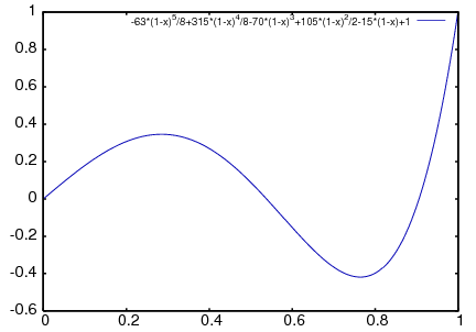
The entire expression legendre_p (5, x) is quoted; this is different than just quoting the function name using 'legendre_p (5, x).

80.1.5 Miscellaneous Functions

The orthopoly package defines the Pochhammer symbol and a unit step function. orthopoly uses the Kronecker delta function and the unit step function in gradef statements.

To convert Pochhammer symbols into quotients of gamma functions, use makegamma.

(%i1) makegamma (pochhammer (x, n));
                          gamma(x + n)
(%o1)                     ------------
                            gamma(x)
(%i2) makegamma (pochhammer (1/2, 1/2));
                                1
(%o2)                       ---------
                            sqrt(%pi)

Derivatives of the Pochhammer symbol are given in terms of the psi function.

(%i1) diff (pochhammer (x, n), x);
(%o1)             (x)  (psi (x + n) - psi (x))
                     n     0             0
(%i2) diff (pochhammer (x, n), n);
(%o2)                   (x)  psi (x + n)
                           n    0

You need to be careful with the expression in (%o1); the difference of the psi functions has polynomials when x = -1, -2, .., -n. These polynomials cancel with factors in pochhammer (x, n) making the derivative a degree n - 1 polynomial when n is a positive integer.

The Pochhammer symbol is defined for negative orders through its representation as a quotient of gamma functions. Consider

(%i1) q : makegamma (pochhammer (x, n));
                          gamma(x + n)
(%o1)                     ------------
                            gamma(x)
(%i2) sublis ([x=11/3, n= -6], q);
                               729
(%o2)                        - ----
                               2240

Alternatively, we can get this result directly.

(%i1) pochhammer (11/3, -6);
                               729
(%o1)                        - ----
                               2240

The unit step function is left-continuous; thus

(%i1) [unit_step (-1/10), unit_step (0), unit_step (1/10)];
(%o1)                       [0, 0, 1]

If you need a unit step function that is neither left or right continuous at zero, define your own using signum; for example,

(%i1) xunit_step (x) := (1 + signum (x))/2$

(%i2) [xunit_step (-1/10), xunit_step (0), xunit_step (1/10)];
                                1
(%o2)                       [0, -, 1]
                                2

Do not redefine unit_step itself; some code in orthopoly requires that the unit step function be left-continuous.

80.1.6 Algorithms

Generally, orthopoly does symbolic evaluation by using a hypergeometic representation of the orthogonal polynomials. The hypergeometic functions are evaluated using the (undocumented) functions hypergeo11 and hypergeo21. The exceptions are the half-integer Bessel functions and the associated Legendre function of the second kind. The half-integer Bessel functions are evaluated using an explicit representation, and the associated Legendre function of the second kind is evaluated using recursion.

For floating point evaluation, we again convert most functions into a hypergeometic form; we evaluate the hypergeometic functions using forward recursion. Again, the exceptions are the half-integer Bessel functions and the associated Legendre function of the second kind. Numerically, the half-integer Bessel functions are evaluated using the SLATEC code.