53.2.1 Scenes

Scene constructor: gr2d (argument_1, ...) ¶

Function gr2d builds an object describing a 2D scene. Arguments are graphic options, graphic objects, or lists containing both graphic options and objects. This scene is interpreted sequentially: graphic options affect those graphic objects placed on its right. Some graphic options affect the global appearance of the scene.

This is the list of graphic objects available for scenes in two dimensions: bars, ellipse, explicit, image, implicit, label, parametric, points, polar, polygon, quadrilateral, rectangle, triangle, vector and geomap (this one defined in package worldmap).

See also draw and draw2d.

(%i1) draw(
    gr2d(
        key="sin (x)",grid=[2,2],
        explicit(
            sin(x),
            x,0,2*%pi
        )
    ),
    gr2d(
        key="cos (x)",grid=[2,2],
        explicit(
            cos(x),
            x,0,2*%pi
        )
    )
 );
(%o1)           [gr2d(explicit), gr2d(explicit)]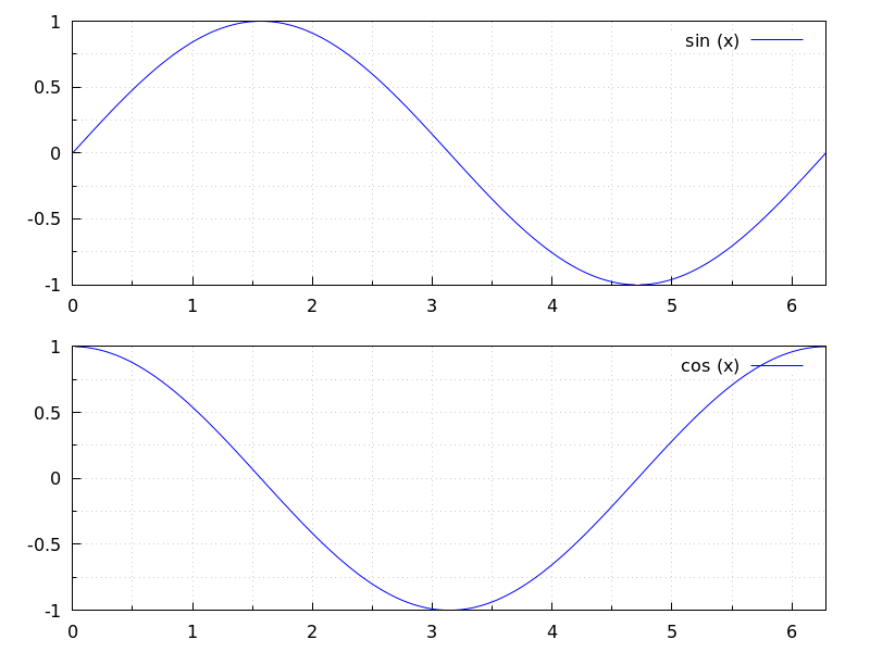

Categories: Package draw ·

Scene constructor: gr3d (argument_1, ...) ¶

Function gr3d builds an object describing a 3d scene. Arguments are graphic options, graphic objects, or lists containing both graphic options and objects. This scene is interpreted sequentially: graphic options affect those graphic objects placed on its right. Some graphic options affect the global appearance of the scene.

This is the list of graphic objects available for scenes in three dimensions:
cylindrical, elevation_grid, explicit, implicit, label, mesh, parametric,
parametric_surface, points, quadrilateral, spherical, triangle, tube,
vector, and geomap (this one defined in package worldmap).

See also draw and draw3d.

Categories: Package draw ·

53.2.2 Functions

Function: draw (<arg_1>, ...) ¶

Plots a series of scenes; its arguments are gr2d and/or gr3d objects, together with some options, or lists of scenes and options. By default, the scenes are put together in one column.

Besides scenes the function draw accepts the following global options: terminal, columns, dimensions, file_name and delay.

Functions draw2d and draw3d short cuts that can be used when only one scene is required, in two or three dimensions, respectively.

See also gr2d and gr3d.

Examples:

(%i1) scene1: gr2d(title="Ellipse",
                   nticks=300,
                   parametric(2*cos(t),5*sin(t),t,0,2*%pi))$
(%i2) scene2: gr2d(title="Triangle",
                   polygon([4,5,7],[6,4,2]))$
(%i3) draw(scene1, scene2, columns = 2)$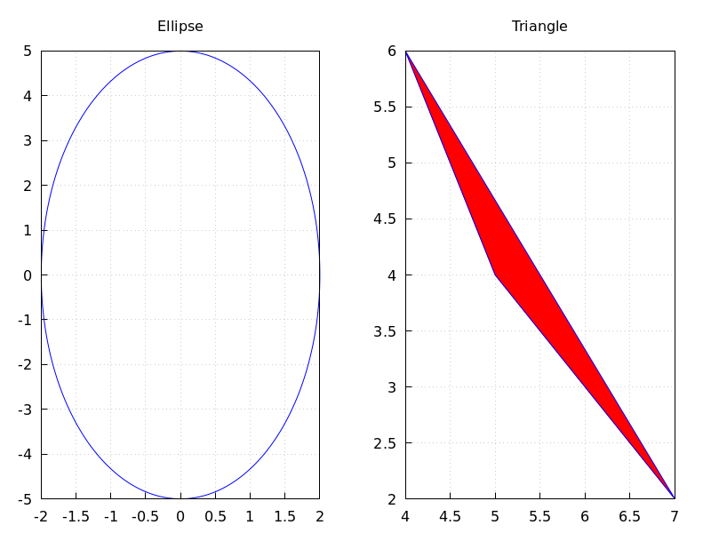

(%i1) scene1: gr2d(title="A sinus",
        grid=true,
        explicit(sin(t),t,0,2*%pi))$
(%i2) scene2: gr2d(title="A cosinus",
        grid=true,
        explicit(cos(t),t,0,2*%pi))$
(%i3) draw(scene1, scene2)$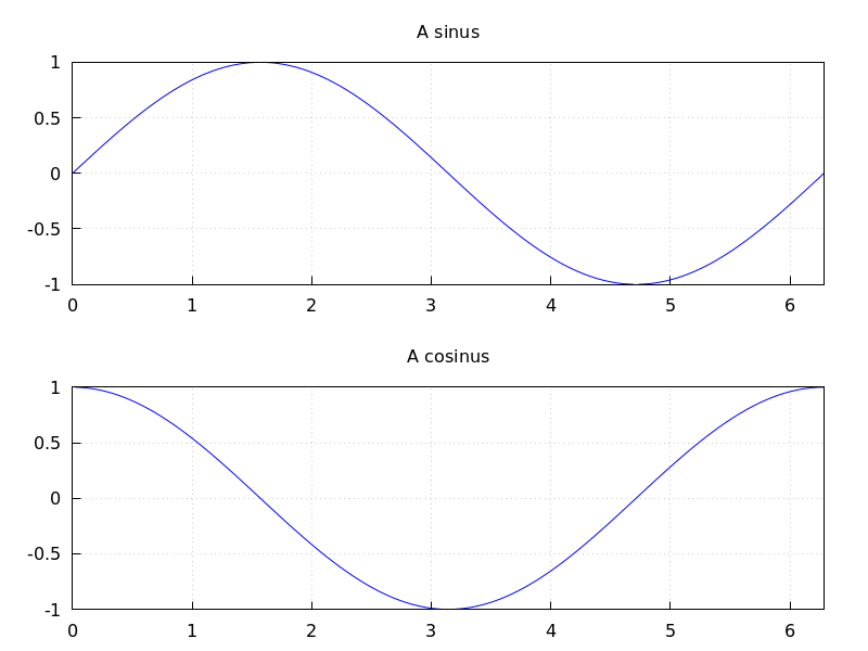

The following two draw sentences are equivalent:

(%i1) draw(gr3d(explicit(x^2+y^2,x,-1,1,y,-1,1)));
(%o1)                          [gr3d(explicit)]
(%i2) draw3d(explicit(x^2+y^2,x,-1,1,y,-1,1));
(%o2)                          [gr3d(explicit)]

Creating an animated gif file:

(%i1) draw(
        delay     = 100,
        file_name = "zzz",
        terminal  = 'animated_gif,
        gr2d(explicit(x^2,x,-1,1)),
        gr2d(explicit(x^3,x,-1,1)),
        gr2d(explicit(x^4,x,-1,1)));
End of animation sequence
(%o1)          [gr2d(explicit), gr2d(explicit), gr2d(explicit)]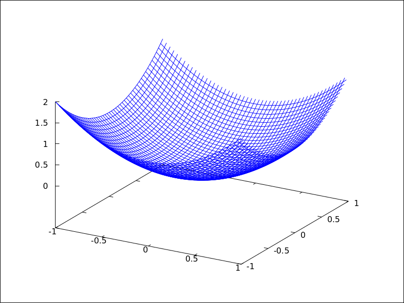

See also gr2d, gr3d, draw2d and draw3d.

Categories: Package draw · File output ·

Function: draw2d (argument_1, ...) ¶

This function is a shortcut for draw(gr2d(options, ..., graphic_object, ...)).

It can be used to plot a unique scene in 2d, as can be seen in most examples below.

See also draw and gr2d.

Categories: Package draw · File output ·

Function: draw3d (argument_1, ...) ¶

This function is a shortcut for draw(gr3d(options, ..., graphic_object, ...)).

It can be used to plot a unique scene in 3d, as can be seen in many examples below.

See also draw and gr3d.

Categories: Package draw · File output ·

Function: draw_file (graphic option, ..., graphic object, ...) ¶

Saves the current plot into a file. Accepted graphics options are: terminal, dimensions and file_name.

Example:

(%i1) /* screen plot */
      draw(gr3d(explicit(x^2+y^2,x,-1,1,y,-1,1)))$
(%i2) /* same plot in eps format */
      draw_file(terminal  = eps,
                dimensions = [5,5]) $

Categories: Package draw · File output ·

Function: multiplot_mode (term) ¶

This function enables Maxima to work in one-window multiplot mode with terminal term; accepted arguments for this function are screen, wxt, aquaterm, windows and none.

When multiplot mode is enabled, each call to draw sends a new plot to the same window, without erasing the previous ones. To disable the multiplot mode, write multiplot_mode(none).

When multiplot mode is enabled, global option terminal is blocked and you have to disable this working mode before changing to another terminal.

On Windows this feature requires Gnuplot 5.0 or newer. Note, that just plotting multiple expressions into the same plot doesn’t require multiplot: It can be done by just issuing multiple explicit or similar commands in a row.

Example:

(%i1) set_draw_defaults(
         xrange = [-1,1],
         yrange = [-1,1],
         grid   = true,
         title  = "Step by step plot" )$
(%i2) multiplot_mode(screen)$
(%i3) draw2d(color=blue,  explicit(x^2,x,-1,1))$
(%i4) draw2d(color=red,   explicit(x^3,x,-1,1))$
(%i5) draw2d(color=brown, explicit(x^4,x,-1,1))$
(%i6) multiplot_mode(none)$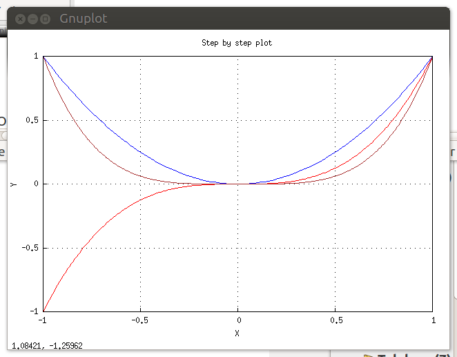

Categories: Package draw · File output ·

Function: set_draw_defaults (graphic option, ..., graphic object, ...) ¶

Sets user graphics options. This function is useful for plotting a sequence of graphics with common graphics options. Calling this function without arguments removes user defaults.

Example:

(%i1) set_draw_defaults(
         xrange = [-10,10],
         yrange = [-2, 2],
         color  = blue,
         grid   = true)$
(%i2) /* plot with user defaults */
      draw2d(explicit(((1+x)**2/(1+x*x))-1,x,-10,10))$
(%i3) set_draw_defaults()$
(%i4) /* plot with standard defaults */
      draw2d(explicit(((1+x)**2/(1+x*x))-1,x,-10,10))$

Categories: Package draw ·

53.2.3 Plot options for draw programs

Graphic option: adapt_depth ¶

Default value: 10

adapt_depth is the maximum number of splittings used by the adaptive plotting routine.

This option is relevant only for 2d explicit functions.

See also nticks

Categories: Package draw ·

Graphic option: allocation ¶

Default value: false

With option allocation it is possible to place a scene in the output window at will; this is of interest in multiplots. When false, the scene is placed automatically, depending on the value assigned to option columns. In any other case, allocation must be set to a list of two pairs of numbers; the first corresponds to the position of the lower left corner of the scene, and the second pair gives the width and height of the plot. All quantities must be given in relative coordinates, between 0 and 1.

Examples:

In site graphics.

(%i1) draw(
        gr2d(
          explicit(x^2,x,-1,1)),
        gr2d(
          allocation = [[1/4, 1/4],[1/2, 1/2]],
          explicit(x^3,x,-1,1),
          grid = true) ) $

Multiplot with selected dimensions.

(%i1) draw(
        terminal = wxt,
        gr2d(
          grid=[5,5],
          allocation = [[0, 0],[1, 1/4]],
          explicit(x^2,x,-1,1)),
        gr3d(
          allocation = [[0, 1/4],[1, 3/4]],
          explicit(x^2+y^2,x,-1,1,y,-1,1) ))$

See also option columns.

Categories: Package draw ·

Graphic option: axis_3d ¶

Default value: true

If axis_3d is true, the x, y and z axis are shown in 3d scenes.

Since this is a global graphics option, its position in the scene description does not matter.

Example:

(%i1) draw3d(axis_3d = false,
             explicit(sin(x^2+y^2),x,-2,2,y,-2,2) )$

See also axis_bottom, axis_left, axis_top, and axis_right for axis in 2d.

Categories: Package draw ·

Graphic option: axis_bottom ¶

Default value: true

If axis_bottom is true, the bottom axis is shown in 2d scenes.

Since this is a global graphics option, its position in the scene description does not matter.

Example:

(%i1) draw2d(axis_bottom = false,
             explicit(x^3,x,-1,1))$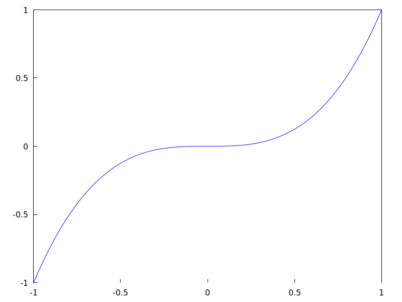

See also axis_left, axis_top, axis_right and axis_3d.

Categories: Package draw ·

Graphic option: axis_left ¶

Default value: true

If axis_left is true, the left axis is shown in 2d scenes.

Since this is a global graphics option, its position in the scene description does not matter.

Example:

(%i1) draw2d(axis_left = false,
             explicit(x^3,x,-1,1))$

See also axis_bottom, axis_top, axis_right and axis_3d.

Categories: Package draw ·

Graphic option: axis_right ¶

Default value: true

If axis_right is true, the right axis is shown in 2d scenes.

Since this is a global graphics option, its position in the scene description does not matter.

Example:

(%i1) draw2d(axis_right = false,
             explicit(x^3,x,-1,1))$

See also axis_bottom, axis_left, axis_top and axis_3d.

Categories: Package draw ·

Graphic option: axis_top ¶

Default value: true

If axis_top is true, the top axis is shown in 2d scenes.

Since this is a global graphics option, its position in the scene description does not matter.

Example:

(%i1) draw2d(axis_top = false,
             explicit(x^3,x,-1,1))$

See also axis_bottom, axis_left, axis_right, and axis_3d.

Categories: Package draw ·

Graphic option: background_color ¶

Default value: white

Sets the background color for terminals. Default background color is white.

Since this is a global graphics option, its position in the scene description does not matter.

This option does not work with terminals epslatex and epslatex_standalone.

See also color

Categories: Package draw ·

Graphic option: border ¶

Default value: true

If border is true, borders of polygons are painted according to line_type and line_width.

This option affects the following graphic objects:

• gr2d: polygon, rectangle and ellipse.

Example:

(%i1) draw2d(color       = brown,
             line_width  = 8,
             polygon([[3,2],[7,2],[5,5]]),
             border      = false,
             fill_color  = blue,
             polygon([[5,2],[9,2],[7,5]]) )$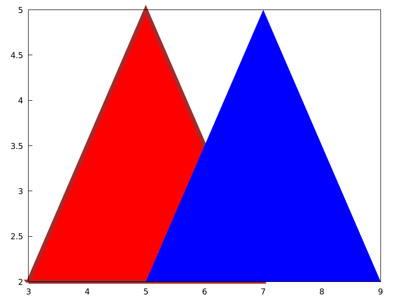

Categories: Package draw ·

Graphic option: capping ¶

Default value: [false, false]

A list with two possible elements, true and false, indicating whether the extremes of a graphic object tube remain closed or open. By default, both extremes are left open.

Setting capping = false is equivalent to capping = [false, false], and capping = true is equivalent to capping = [true, true].

Example:

(%i1) draw3d(
        capping = [false, true],
        tube(0, 0, a, 1,
             a, 0, 8) )$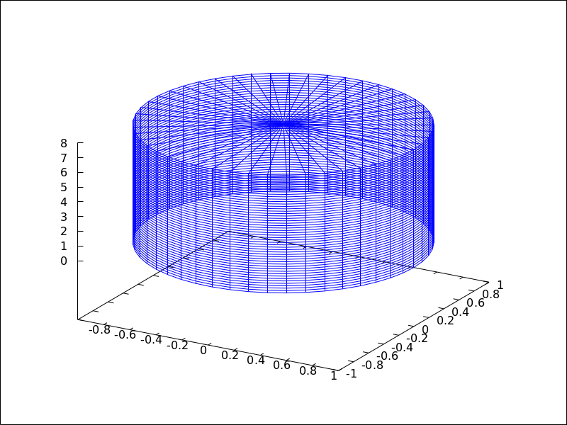

Categories: Package draw ·

Graphic option: cbrange ¶

Default value: auto

If cbrange is auto, the range for the values which are colored when enhanced3d is not false is computed automatically. Values outside of the color range use color of the nearest extreme.

When enhanced3d or colorbox is false, option cbrange has no effect.

If the user wants a specific interval for the colored values, it must be given as a Maxima list, as in cbrange=[-2, 3].

Since this is a global graphics option, its position in the scene description does not matter.

Example:

(%i1) draw3d (
        enhanced3d     = true,
        color          = green,
        cbrange = [-3,10],
        explicit(x^2+y^2, x,-2,2,y,-2,2)) $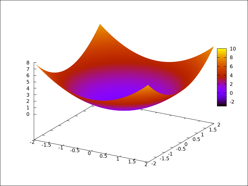

See also enhanced3d, colorbox and cbtics.

Categories: Package draw ·

Graphic option: cbtics ¶

Default value: auto

This graphic option controls the way tic marks are drawn on the colorbox when option enhanced3d is not false.

When enhanced3d or colorbox is false, option cbtics has no effect.

See xtics for a complete description.

Example :

(%i1) draw3d (
        enhanced3d = true,
        color      = green,
        cbtics  = {["High",10],["Medium",05],["Low",0]},
        cbrange = [0, 10],
        explicit(x^2+y^2, x,-2,2,y,-2,2)) $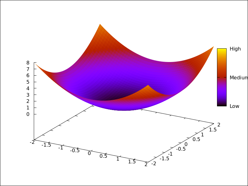

See also enhanced3d, colorbox and cbrange.

Categories: Package draw ·

Graphic option: color ¶

Default value: blue

color specifies the color for plotting lines, points, borders of polygons and labels.

Colors can be given as names or in hexadecimal rgb code. If a gnuplot version >= 5.0 is used and the terminal that is in use supports this rgba colors with transparency information are also supported.

Available color names are:

white            black            gray0            grey0 
gray10           grey10           gray20           grey20     
gray30           grey30           gray40           grey40     
gray50           grey50           gray60           grey60     
gray70           grey70           gray80           grey80
gray90           grey90           gray100          grey100 
gray             grey             light_gray       light_grey 
dark_gray        dark_grey        red              light_red 
dark_red         yellow           light_yellow     dark_yellow
green            light_green      dark_green       spring_green
forest_green     sea_green        blue             light_blue 
dark_blue        midnight_blue    navy             medium_blue 
royalblue        skyblue          cyan             light_cyan 
dark_cyan        magenta          light_magenta    dark_magenta
turquoise        light_turquoise  dark_turquoise   pink 
light_pink       dark_pink        coral            light_coral 
orange_red       salmon           light_salmon     dark_salmon 
aquamarine       khaki            dark_khaki       goldenrod 
light_goldenrod  dark_goldenrod   gold             beige 
brown            orange           dark_orange      violet 
dark_violet      plum             purple

Cromatic components in hexadecimal code are introduced in the form "#rrggbb".

Example:

(%i1) draw2d(explicit(x^2,x,-1,1), /* default is black */
             color = red,
             explicit(0.5 + x^2,x,-1,1),
             color = blue,
             explicit(1 + x^2,x,-1,1),
             color = light_blue,
             explicit(1.5 + x^2,x,-1,1),
             color = "#23ab0f",
             label(["This is a label",0,1.2])  )$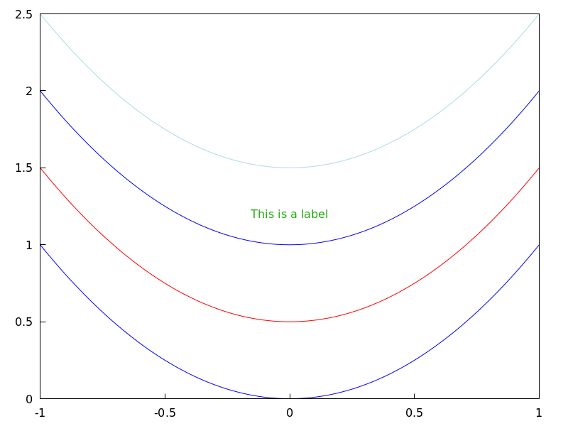

(%i1) draw2d(
             line_width=50,
             color="#FF0000",
             explicit(sin(x),x,0,10),
             color="#0000FF80",
             explicit(cos(x),x,0,10)
      );

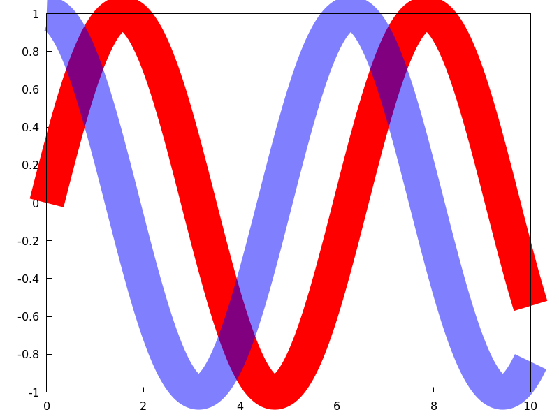
(%i1) H(p,p_0) := %i/(2*%pi*(p-p_0))$
(%i2) draw2d(
       proportional_axes=xy,
       ip_grid=[150,150],
       grid=true,
       makelist(
         [
           color=printf(false,"#~2,'0x~2,'0x~2,'0x",i*10,0,0),
           key_pos=top_left,
           key = if mod(i,5)=0 then sconcat("H=",i,"A/M") else "",
           implicit(
             cabs(H(x+%i*y,-1-%i)+H(x+%i*y,1+%i)-H(x+%i*y,1-%i)
                  -H(x+%i*y,-1+%i))=i/10,
             x,-3,3,
             y,-3,3
           )
         ],
         i,1,25
       )
      )$

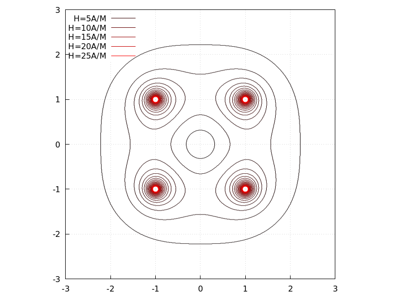
(%i1) draw2d(
        "figures/draw_color4",
        makelist(
            [
                color=i,
                key=sconcat("color =",i),
                explicit(sin(i*x),x,0,1)
            ],
            i,0,17
        )
    )$

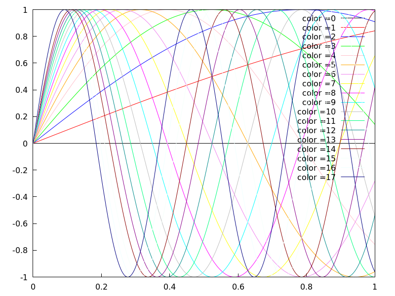
See also fill_color.

Categories: Package draw ·

Graphic option: colorbox ¶

Default value: true

If colorbox is true, a color scale without label is drawn together with image 2D objects, or coloured 3d objects. If colorbox is false, no color scale is shown. If colorbox is a string, a color scale with label is drawn.

Since this is a global graphics option, its position in the scene description does not matter.

Example:

Color scale and images.

(%i1) im: apply('matrix,
                 makelist(makelist(random(200),i,1,30),i,1,30))$
(%i2) draw(
          gr2d(image(im,0,0,30,30)),
          gr2d(colorbox = false, image(im,0,0,30,30))
      )$

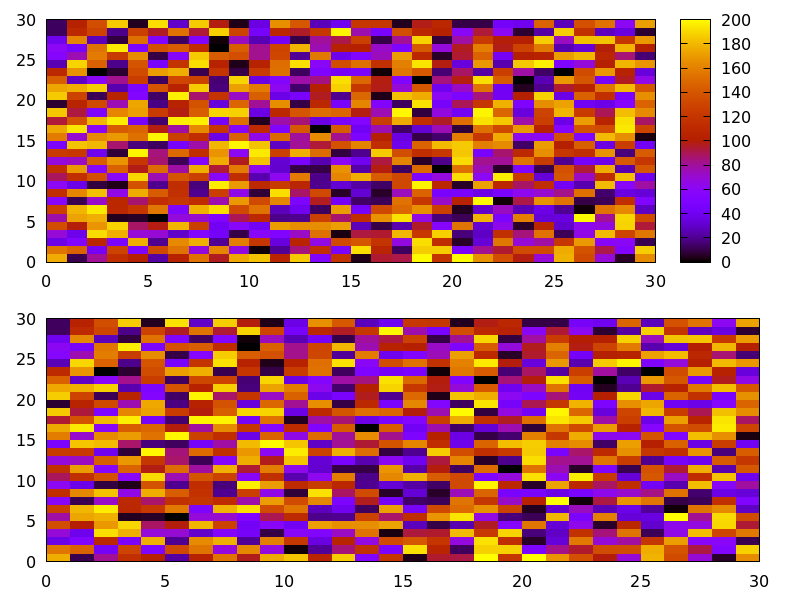
Color scale and 3D coloured object.

(%i1) draw3d(
        colorbox   = "Magnitude",
        enhanced3d = true,
        explicit(x^2+y^2,x,-1,1,y,-1,1))$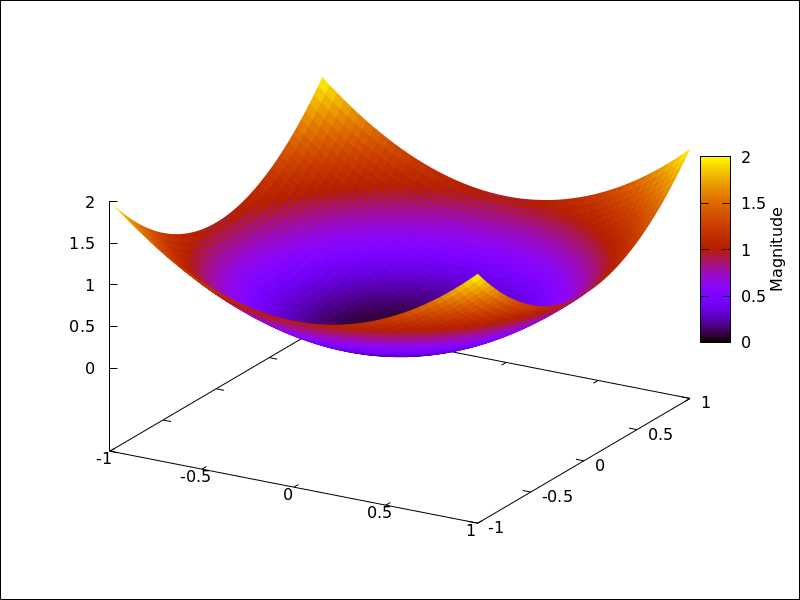

See also palette_draw.

Categories: Package draw ·

Graphic option: columns ¶

Default value: 1

columns is the number of columns in multiple plots.

Since this is a global graphics option, its position in the scene description does not matter. It can be also used as an argument of function draw.

Example:

(%i1) scene1: gr2d(title="Ellipse",
                   nticks=30,
                   parametric(2*cos(t),5*sin(t),t,0,2*%pi))$
(%i2) scene2: gr2d(title="Triangle",
                   polygon([4,5,7],[6,4,2]))$
(%i3) draw(scene1, scene2, columns = 2)$

Categories: Package draw ·

Graphic option: contour ¶

Default value: none

Option contour enables the user to select where to plot contour lines. Possible values are:

• none: no contour lines are plotted.
• base: contour lines are projected on the xy plane.
• surface: contour lines are plotted on the surface.
• both: two contour lines are plotted: on the xy plane and on the surface.
• map: contour lines are projected on the xy plane, and the view point is set just in the vertical.

Since this is a global graphics option, its position in the scene description does not matter.

Example:

(%i1) draw3d(explicit(20*exp(-x^2-y^2)-10,x,0,2,y,-3,3),
             contour_levels = 15,
             contour        = both,
             surface_hide   = true) $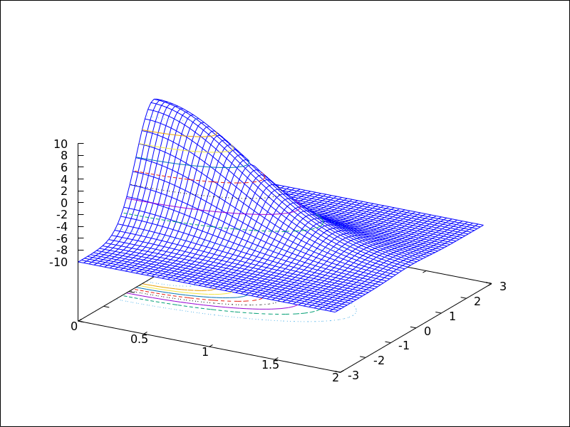

(%i1) draw3d(explicit(20*exp(-x^2-y^2)-10,x,0,2,y,-3,3),
             contour_levels = 15,
             contour        = map
      ) $

Categories: Package draw ·

Graphic option: contour_levels ¶

Default value: 5

This graphic option controls the way contours are drawn. contour_levels can be set to a positive integer number, a list of three numbers or an arbitrary set of numbers:

• When option contour_levels is bounded to positive integer n, n contour lines will be drawn at equal intervals. By default, five equally spaced contours are plotted.
• When option contour_levels is bounded to a list of length three of the form [lowest,s,highest], contour lines are plotted from lowest to highest in steps of s.
• When option contour_levels is bounded to a set of numbers of the form {n1, n2, ...}, contour lines are plotted at values n1, n2, ...

Since this is a global graphics option, its position in the scene description does not matter.

Examples:

Ten equally spaced contour lines. The actual number of levels can be adjusted to give simple labels.

(%i1) draw3d(color = green,
             explicit(20*exp(-x^2-y^2)-10,x,0,2,y,-3,3),
             contour_levels = 10,
             contour        = both,
             surface_hide   = true) $

From -8 to 8 in steps of 4.

(%i1) draw3d(color = green,
             explicit(20*exp(-x^2-y^2)-10,x,0,2,y,-3,3),
             contour_levels = [-8,4,8],
             contour        = both,
             surface_hide   = true) $

Isolines at levels -7, -6, 0.8 and 5.

(%i1) draw3d(color = green,
             explicit(20*exp(-x^2-y^2)-10,x,0,2,y,-3,3),
             contour_levels = {-7, -6, 0.8, 5},
             contour        = both,
             surface_hide   = true) $

See also contour.

Categories: Package draw ·

Graphic option: data_file_name ¶

Default value: "data.gnuplot"

This is the name of the file with the numeric data needed by Gnuplot to build the requested plot.

Since this is a global graphics option, its position in the scene description does not matter. It can be also used as an argument of function draw.

See example in gnuplot_file_name.

Categories: Package draw ·

Graphic option: delay ¶

Default value: 5

This is the delay in 1/100 seconds of frames in animated gif files.

Since this is a global graphics option, its position in the scene description does not matter. It can be also used as an argument of function draw.

Example:

(%i1) draw(
        delay     = 100,
        file_name = "zzz",
        terminal  = 'animated_gif,
        gr2d(explicit(x^2,x,-1,1)),
        gr2d(explicit(x^3,x,-1,1)),
        gr2d(explicit(x^4,x,-1,1)));
End of animation sequence
(%o2)          [gr2d(explicit), gr2d(explicit), gr2d(explicit)]

Option delay is only active in animated gif’s; it is ignored in any other case.

See also terminal, and dimensions.

Categories: Package draw ·

Graphic option: dimensions ¶

Default value: [600,500]

Dimensions of the output terminal. Its value is a list formed by the width and the height. The meaning of the two numbers depends on the terminal you are working with.

With terminals gif, animated_gif, png, jpg, svg, screen, wxt, and aquaterm, the integers represent the number of points in each direction. If they are not integers, they are rounded.

With terminals eps, eps_color, pdf, and pdfcairo, both numbers represent hundredths of cm, which means that, by default, pictures in these formats are 6 cm in width and 5 cm in height.

Since this is a global graphics option, its position in the scene description does not matter. It can be also used as an argument of function draw.

Examples:

Option dimensions applied to file output and to wxt canvas.

(%i1) draw2d(
        dimensions = [300,300],
        terminal   = 'png,
        explicit(x^4,x,-1,1)) $
(%i2) draw2d(
        dimensions = [300,300],
        terminal   = 'wxt,
        explicit(x^4,x,-1,1)) $

Option dimensions applied to eps output. We want an eps file with A4 portrait dimensions.

(%i1) A4portrait: 100*[21, 29.7]$
(%i2) draw3d(
        dimensions = A4portrait,
        terminal   = 'eps,
        explicit(x^2-y^2,x,-2,2,y,-2,2)) $

Categories: Package draw ·

Graphic option: draw_realpart ¶

Default value: true

When true, functions to be drawn are considered as complex functions whose real part value should be plotted; when false, nothing will be plotted when the function does not give a real value.

This option affects objects explicit and parametric in 2D and 3D, and parametric_surface.

Example:

(%i1) draw2d(
        draw_realpart = false,
        explicit(sqrt(x^2  - 4*x) - x, x, -1, 5),
        color         = red,
        draw_realpart = true,
        parametric(x,sqrt(x^2  - 4*x) - x + 1, x, -1, 5) );

Categories: Package draw ·

Graphic option: enhanced3d ¶

Default value: none

If enhanced3d is none, surfaces are not colored in 3D plots. In order to get a colored surface, a list must be assigned to option enhanced3d, where the first element is an expression and the rest are the names of the variables or parameters used in that expression. A list such [f(x,y,z), x, y, z] means that point [x,y,z] of the surface is assigned number f(x,y,z), which will be colored according to the actual palette. For those 3D graphic objects defined in terms of parameters, it is possible to define the color number in terms of the parameters, as in [f(u), u], as in objects parametric and tube, or [f(u,v), u, v], as in object parametric_surface. While all 3D objects admit the model based on absolute coordinates, [f(x,y,z), x, y, z], only two of them, namely explicit and elevation_grid, accept also models defined on the [x,y] coordinates, [f(x,y), x, y]. 3D graphic object implicit accepts only the [f(x,y,z), x, y, z] model. Object points accepts also the [f(x,y,z), x, y, z] model, but when points have a chronological nature, model [f(k), k] is also valid, being k an ordering parameter.

When enhanced3d is assigned something different to none, options color and surface_hide are ignored.

The names of the variables defined in the lists may be different to those used in the definitions of the graphic objects.

In order to maintain back compatibility, enhanced3d = false is equivalent to enhanced3d = none, and enhanced3d = true is equivalent to enhanced3d = [z, x, y, z]. If an expression is given to enhanced3d, its variables must be the same used in the surface definition. This is not necessary when using lists.

See option palette to learn how palettes are specified.

Examples:

explicit object with coloring defined by the [f(x,y,z), x, y, z] model.

(%i1) draw3d(
         enhanced3d = [x-z/10,x,y,z],
         palette    = gray,
         explicit(20*exp(-x^2-y^2)-10,x,-3,3,y,-3,3))$

explicit object with coloring defined by the [f(x,y), x, y] model. The names of the variables defined in the lists may be different to those used in the definitions of the graphic objects; in this case, r corresponds to x, and s to y.

(%i1) draw3d(
         enhanced3d = [sin(r*s),r,s],
         explicit(20*exp(-x^2-y^2)-10,x,-3,3,y,-3,3))$

parametric object with coloring defined by the [f(x,y,z), x, y, z] model.

(%i1) draw3d(
         nticks = 100,
         line_width = 2,
         enhanced3d = [if y>= 0 then 1 else 0, x, y, z],
         parametric(sin(u)^2,cos(u),u,u,0,4*%pi)) $

parametric object with coloring defined by the [f(u), u] model. In this case, (u-1)^2 is a shortcut for [(u-1)^2,u].

(%i1) draw3d(
         nticks = 60,
         line_width = 3,
         enhanced3d = (u-1)^2,
         parametric(cos(5*u)^2,sin(7*u),u-2,u,0,2))$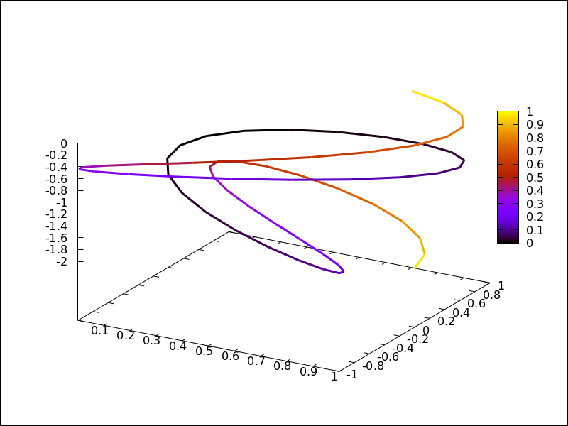

elevation_grid object with coloring defined by the [f(x,y), x, y] model.

(%i1) m: apply(
           matrix,
           makelist(makelist(cos(i^2/80-k/30),k,1,30),i,1,20)) $
(%i2) draw3d(
         enhanced3d = [cos(x*y*10),x,y],
         elevation_grid(m,-1,-1,2,2),
         xlabel = "x",
         ylabel = "y");

tube object with coloring defined by the [f(x,y,z), x, y, z] model.

(%i1) draw3d(
         enhanced3d = [cos(x-y),x,y,z],
         palette = gray,
         xu_grid = 50,
         tube(cos(a), a, 0, 1, a, 0, 4*%pi) )$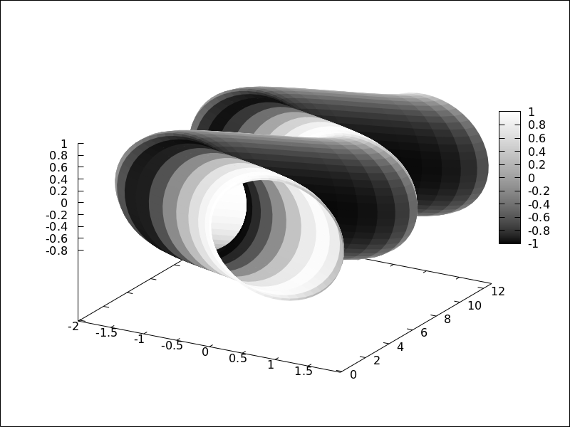

tube object with coloring defined by the [f(u), u] model. Here, enhanced3d = -a would be the shortcut for enhanced3d = [-foo,foo].

(%i1) draw3d(
         capping = [true, false],
         palette = [26,15,-2],
         enhanced3d = [-foo, foo],
         tube(a, a, a^2, 1, a, -2, 2) )$

implicit and points objects with coloring defined by the [f(x,y,z), x, y, z] model.

(%i1) draw3d(
         enhanced3d = [x-y,x,y,z],
         implicit((x^2+y^2+z^2-1)*(x^2+(y-1.5)^2+z^2-0.5)=0.015,
                  x,-1,1,y,-1.2,2.3,z,-1,1)) $
(%i2) m: makelist([random(1.0),random(1.0),random(1.0)],k,1,2000)$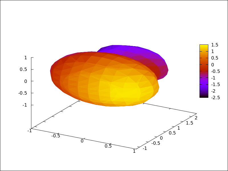

(%i3) draw3d(
         point_type = filled_circle,
         point_size = 2,
         enhanced3d = [u+v-w,u,v,w],
         points(m) ) $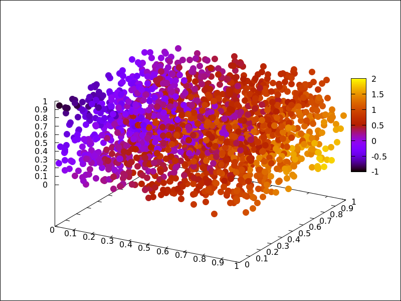

When points have a chronological nature, model [f(k), k] is also valid, being k an ordering parameter.

(%i1) m:makelist([random(1.0), random(1.0), random(1.0)],k,1,5)$
(%i2) draw3d(
         enhanced3d = [sin(j), j],
         point_size = 3,
         point_type = filled_circle,
         points_joined = true,
         points(m)) $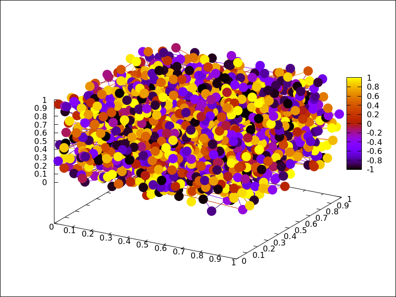

Categories: Package draw ·

Graphic option: error_type ¶

Default value: y

Depending on its value, which can be x, y, or xy, graphic object errors will draw points with horizontal, vertical, or both, error bars. When error_type=boxes, boxes will be drawn instead of crosses.

See also errors.

Graphic option: file_name ¶

Default value: "maxima_out"

This is the name of the file where terminals png, jpg, gif, eps, eps_color, pdf, pdfcairo and svg will save the graphic.

Since this is a global graphics option, its position in the scene description does not matter. It can be also used as an argument of function draw.

Example:

(%i1) draw2d(file_name = "myfile",
             explicit(x^2,x,-1,1),
             terminal  = 'png)$

See also terminal, dimensions_draw.

Categories: Package draw ·

Graphic option: fill_color ¶

Default value: "red"

fill_color specifies the color for filling polygons and 2d explicit functions.

See color to learn how colors are specified.

Categories: Package draw ·

Graphic option: fill_density ¶

Default value: 0

fill_density is a number between 0 and 1 that specifies the intensity of the fill_color in bars objects.

See bars for examples.

Graphic option: filled_func ¶

Default value: false

Option filled_func controls how regions limited by functions should be filled. When filled_func is true, the region bounded by the function defined with object explicit and the bottom of the graphic window is filled with fill_color. When filled_func contains a function expression, then the region bounded by this function and the function defined with object explicit will be filled. By default, explicit functions are not filled.

A useful special case is filled_func=0, which generates the region bond by the horizontal axis and the explicit function.

This option affects only the 2d graphic object explicit.

Example:

Region bounded by an explicit object and the bottom of the graphic window.

(%i1) draw2d(fill_color  = red,
             filled_func = true,
             explicit(sin(x),x,0,10) )$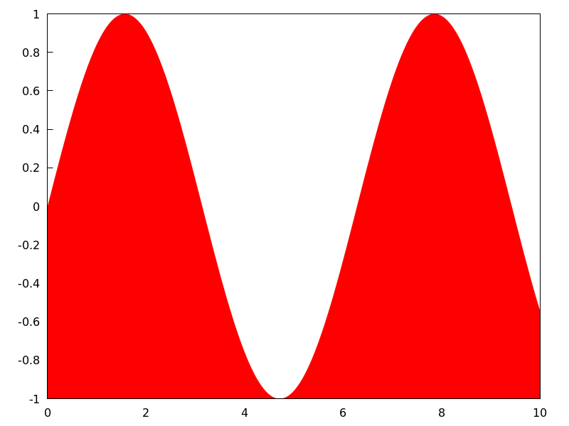

Region bounded by an explicit object and the function defined by option filled_func. Note that the variable in filled_func must be the same as that used in explicit.

(%i1) draw2d(fill_color  = grey,
             filled_func = sin(x),
             explicit(-sin(x),x,0,%pi));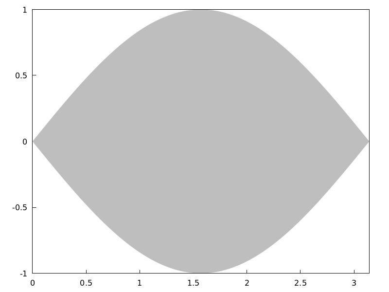

See also fill_color and explicit.

Categories: Package draw ·

Graphic option: font ¶

Default value: "" (empty string)

This option can be used to set the font face to be used by the terminal. Only one font face and size can be used throughout the plot.

Since this is a global graphics option, its position in the scene description does not matter.

See also font_size.

Gnuplot doesn’t handle fonts by itself, it leaves this task to the support libraries of the different terminals, each one with its own philosophy about it. A brief summary follows:

• x11: Uses the normal x11 font server mechanism.

  Example:

  (%i1) draw2d(font      = "Arial", 
               font_size = 20,
               label(["Arial font, size 20",1,1]))$
  

• windows: The windows terminal doesn’t support changing of fonts from inside the plot. Once the plot has been generated, the font can be changed right-clicking on the menu of the graph window.
• png, jpeg, gif: The libgd library uses the font path stored in the environment variable GDFONTPATH; in this case, it is only necessary to set option font to the font’s name. It is also possible to give the complete path to the font file.

  Examples:

  Option font can be given the complete path to the font file:

  (%i1) path: "/usr/share/fonts/truetype/freefont/" $
  (%i2) file: "FreeSerifBoldItalic.ttf" $
  (%i3) draw2d(
          font      = concat(path, file), 
          font_size = 20,
          color     = red,
          label(["FreeSerifBoldItalic font, size 20",1,1]),
          terminal  = png)$
  

  If environment variable GDFONTPATH is set to the path where font files are allocated, it is possible to set graphic option font to the name of the font.

  (%i1) draw2d(
          font      = "FreeSerifBoldItalic", 
          font_size = 20,
          color     = red,
          label(["FreeSerifBoldItalic font, size 20",1,1]),
          terminal  = png)$
  

• Postscript: Standard Postscript fonts are:
  "Times-Roman", "Times-Italic", "Times-Bold", "Times-BoldItalic",
  "Helvetica", "Helvetica-Oblique", "Helvetica-Bold",
  "Helvetic-BoldOblique", "Courier", "Courier-Oblique", "Courier-Bold",
  and "Courier-BoldOblique".

  Example:

  (%i1) draw2d(
          font      = "Courier-Oblique", 
          font_size = 15,
          label(["Courier-Oblique font, size 15",1,1]),
          terminal = eps)$
  

• pdf: Uses same fonts as Postscript.
• pdfcairo: Uses same fonts as wxt.
• wxt: The pango library finds fonts via the fontconfig utility.
• aqua: Default is "Times-Roman".

The gnuplot documentation is an important source of information about terminals and fonts.

Categories: Package draw ·

Graphic option: font_size ¶

Default value: 10

This option can be used to set the font size to be used by the terminal. Only one font face and size can be used throughout the plot. font_size is active only when option font is not equal to the empty string.

Since this is a global graphics option, its position in the scene description does not matter.

See also font.

Categories: Package draw ·

Graphic option: gnuplot_file_name ¶

Default value: "maxout_xxx.gnuplot" with "xxx" being a number that is unique to each concurrently-running maxima process.

This is the name of the file with the necessary commands to be processed by Gnuplot.

Since this is a global graphics option, its position in the scene description does not matter. It can be also used as an argument of function draw.

Example:

(%i1) draw2d(
       file_name = "my_file",
       gnuplot_file_name = "my_commands_for_gnuplot",
       data_file_name    = "my_data_for_gnuplot",
       terminal          = png,
       explicit(x^2,x,-1,1)) $

See also data_file_name.

Categories: Package draw ·

Graphic option: grid ¶

Default value: false

If grid is not false, a grid will be drawn on the xy plane. If grid is assigned true, one grid line per tick of each axis is drawn. If grid is assigned a list nx,ny with [nx,ny] > [0,0] instead nx lines per tick of the x axis and ny lines per tick of the y axis are drawn.

Since this is a global graphics option, its position in the scene description does not matter.

Example:

(%i1) draw2d(grid = true,
             explicit(exp(u),u,-2,2))$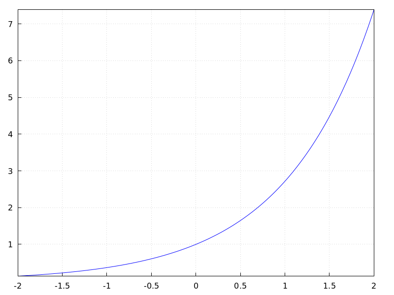

(%i1) draw2d(grid = [2,2],
             explicit(sin(x),x,0,2*%pi))$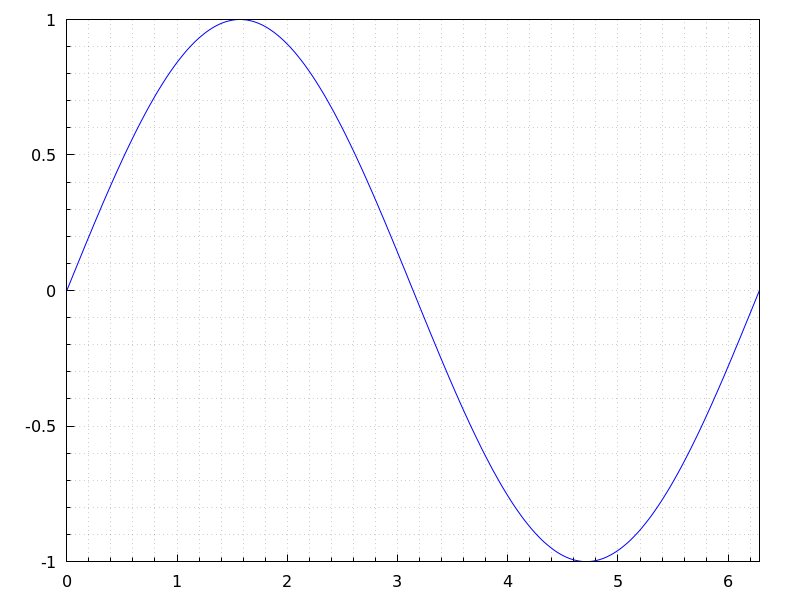

Categories: Package draw ·

Graphic option: head_angle ¶

Default value: 45

head_angle indicates the angle, in degrees, between the arrow heads and the segment.

This option is relevant only for vector objects.

Example:

(%i1) draw2d(xrange      = [0,10],
             yrange      = [0,9],
             head_length = 0.7,
             head_angle  = 10,
             vector([1,1],[0,6]),
             head_angle  = 20,
             vector([2,1],[0,6]),
             head_angle  = 30,
             vector([3,1],[0,6]),
             head_angle  = 40,
             vector([4,1],[0,6]),
             head_angle  = 60,
             vector([5,1],[0,6]),
             head_angle  = 90,
             vector([6,1],[0,6]),
             head_angle  = 120,
             vector([7,1],[0,6]),
             head_angle  = 160,
             vector([8,1],[0,6]),
             head_angle  = 180,
             vector([9,1],[0,6]) )$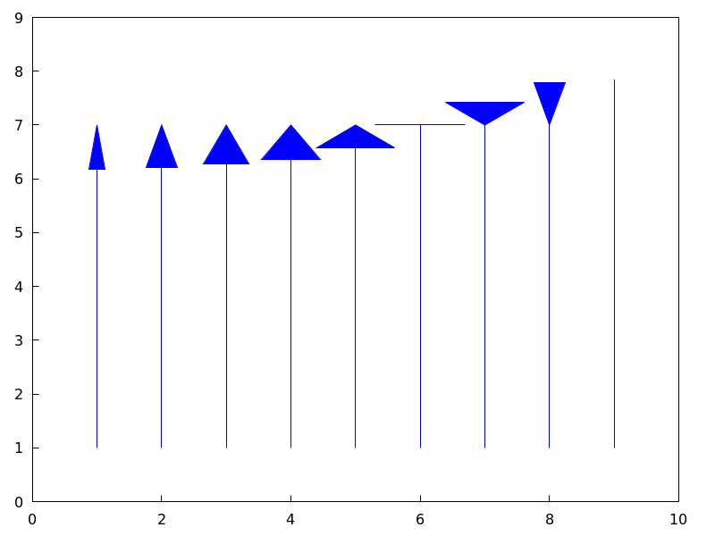

See also head_both, head_length, and head_type.

Categories: Package draw ·

Graphic option: head_both ¶

Default value: false

If head_both is true, vectors are plotted with two arrow heads. If false, only one arrow is plotted.

This option is relevant only for vector objects.

Example:

(%i1) draw2d(xrange      = [0,8],
             yrange      = [0,8],
             head_length = 0.7,
             vector([1,1],[6,0]),
             head_both   = true,
             vector([1,7],[6,0]) )$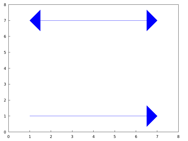

See also head_length, head_angle, and head_type.

Categories: Package draw ·

Graphic option: head_length ¶

Default value: 2

head_length indicates, in x-axis units, the length of arrow heads.

This option is relevant only for vector objects.

Example:

(%i1) draw2d(xrange      = [0,12],
             yrange      = [0,8],
             vector([0,1],[5,5]),
             head_length = 1,
             vector([2,1],[5,5]),
             head_length = 0.5,
             vector([4,1],[5,5]),
             head_length = 0.25,
             vector([6,1],[5,5]))$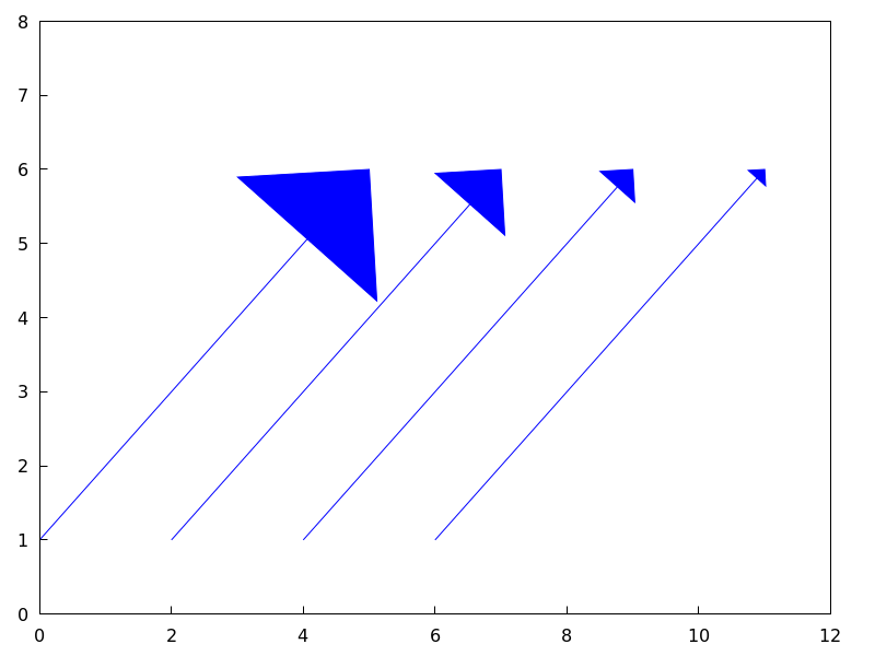

See also head_both, head_angle, and head_type.

Categories: Package draw ·

Graphic option: head_type ¶

Default value: filled

head_type is used to specify how arrow heads are plotted. Possible values are: filled (closed and filled arrow heads), empty (closed but not filled arrow heads), and nofilled (open arrow heads).

This option is relevant only for vector objects.

Example:

(%i1) draw2d(xrange      = [0,12],
             yrange      = [0,10],
             head_length = 1,
             vector([0,1],[5,5]), /* default type */
             head_type = 'empty,
             vector([3,1],[5,5]),
             head_type = 'nofilled,
             vector([6,1],[5,5]))$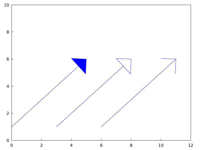

See also head_both, head_angle, and head_length.

Categories: Package draw ·

Graphic option: interpolate_color ¶

Default value: false

This option is relevant only when enhanced3d is not false.

When interpolate_color is false, surfaces are colored with homogeneous quadrangles. When true, color transitions are smoothed by interpolation.

interpolate_color also accepts a list of two numbers, [m,n]. For positive m and n, each quadrangle or triangle is interpolated m times and n times in the respective direction. For negative m and n, the interpolation frequency is chosen so that there will be at least |m| and |n| points drawn; you can consider this as a special gridding function. Zeros, i.e. interpolate_color=[0,0], will automatically choose an optimal number of interpolated surface points.

Also, interpolate_color=true is equivalent to interpolate_color=[0,0].

Examples:

Color interpolation with explicit functions.

(%i1) draw3d(
        enhanced3d   = sin(x*y),
        explicit(20*exp(-x^2-y^2)-10, x ,-3, 3, y, -3, 3)) $

(%i2) draw3d(
        interpolate_color = true,
        enhanced3d   = sin(x*y),
        explicit(20*exp(-x^2-y^2)-10, x ,-3, 3, y, -3, 3)) $

(%i3) draw3d(
        interpolate_color = [-10,0],
        enhanced3d   = sin(x*y),
        explicit(20*exp(-x^2-y^2)-10, x ,-3, 3, y, -3, 3)) $

Color interpolation with the mesh graphic object.

Interpolating colors in parametric surfaces can give unexpected results.

(%i1) draw3d( 
        enhanced3d = true,
        mesh([[1,1,3],   [7,3,1],[12,-2,4],[15,0,5]],
             [[2,7,8],   [4,3,1],[10,5,8], [12,7,1]],
             [[-2,11,10],[6,9,5],[6,15,1], [20,15,2]])) $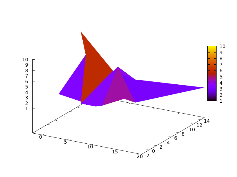

(%i2) draw3d( 
        enhanced3d        = true,
        interpolate_color = true,
        mesh([[1,1,3],   [7,3,1],[12,-2,4],[15,0,5]],
             [[2,7,8],   [4,3,1],[10,5,8], [12,7,1]],
             [[-2,11,10],[6,9,5],[6,15,1], [20,15,2]])) $

(%i3) draw3d( 
        enhanced3d        = true,
        interpolate_color = true,
        view=map,
        mesh([[1,1,3],   [7,3,1],[12,-2,4],[15,0,5]],
             [[2,7,8],   [4,3,1],[10,5,8], [12,7,1]],
             [[-2,11,10],[6,9,5],[6,15,1], [20,15,2]])) $

See also enhanced3d.

Categories: Package draw ·

Graphic option: ip_grid ¶

Default value: [50, 50]

ip_grid sets the grid for the first sampling in implicit plots.

This option is relevant only for implicit objects.

Categories: Package draw ·

Graphic option: ip_grid_in ¶

Default value: [5, 5]

ip_grid_in sets the grid for the second sampling in implicit plots.

This option is relevant only for implicit objects.

Categories: Package draw ·

Graphic option: key ¶

Default value: "" (empty string)

key is the name of a function in the legend. If key is an empty string, no key is assigned to the function.

This option affects the following graphic objects:

• gr2d: points, polygon, rectangle, ellipse, vector, explicit, implicit, parametric and polar.
• gr3d: points, explicit, parametric and parametric_surface.

Example:

(%i1) draw2d(key   = "Sinus",
             explicit(sin(x),x,0,10),
             key   = "Cosinus",
             color = red,
             explicit(cos(x),x,0,10) )$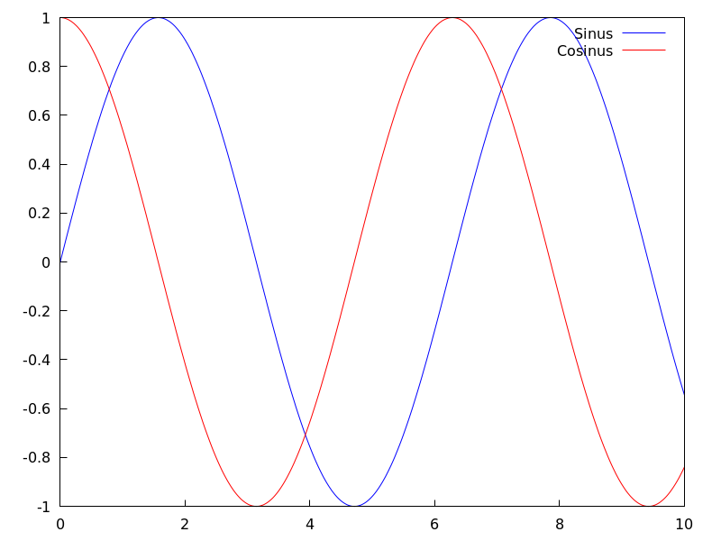

Categories: Package draw ·

Graphic option: key_pos ¶

Default value: "" (empty string)

key_pos defines at which position the legend will be drawn. If key is an empty string, "top_right" is used. Available position specifiers are: top_left, top_center, top_right, center_left, center, center_right, bottom_left, bottom_center, and bottom_right.

Since this is a global graphics option, its position in the scene description does not matter.

Example:

(%i1) draw2d(
        key_pos = top_left,
        key   = "x",
        explicit(x,  x,0,10),
        color= red,
        key   = "x squared",
        explicit(x^2,x,0,10))$
(%i3) draw3d(
        key_pos = center,
        key   = "x",
        explicit(x+y,x,0,10,y,0,10),
        color= red,
        key   = "x squared",
        explicit(x^2+y^2,x,0,10,y,0,10))$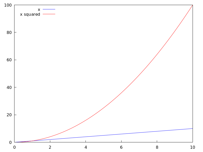

Categories: Package draw ·

Graphic option: label_alignment ¶

Default value: center

label_alignment is used to specify where to write labels with respect to the given coordinates. Possible values are: center, left, and right.

This option is relevant only for label objects.

Example:

(%i1) draw2d(xrange          = [0,10],
             yrange          = [0,10],
             points_joined   = true,
             points([[5,0],[5,10]]),
             color           = blue,
             label(["Centered alignment (default)",5,2]),
             label_alignment = 'left,
             label(["Left alignment",5,5]),
             label_alignment = 'right,
             label(["Right alignment",5,8]))$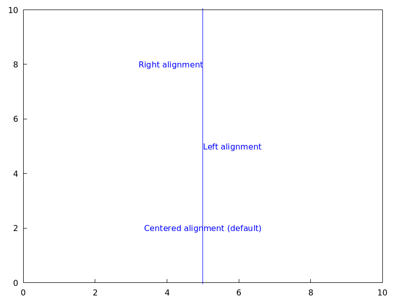

See also label_orientation, and color

Categories: Package draw ·

Graphic option: label_orientation ¶

Default value: horizontal

label_orientation is used to specify orientation of labels. Possible values are: horizontal, and vertical.

This option is relevant only for label objects.

Example:

In this example, a dummy point is added to get an image. Package draw needs always data to draw an scene.

(%i1) draw2d(xrange     = [0,10],
             yrange     = [0,10],
             point_size = 0,
             points([[5,5]]),
             color      = navy,
             label(["Horizontal orientation (default)",5,2]),
             label_orientation = 'vertical,
             color             = "#654321",
             label(["Vertical orientation",1,5]))$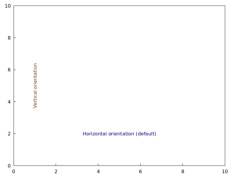

See also label_alignment and color

Categories: Package draw ·

Graphic option: line_type ¶

Default value: solid

line_type indicates how lines are displayed; possible values are solid and dots, both available in all terminals, and dashes, short_dashes, short_long_dashes, short_short_long_dashes, and dot_dash, which are not available in png, jpg, and gif terminals.

This option affects the following graphic objects:

• gr2d: points, polygon, rectangle, ellipse, vector, explicit, implicit, parametric and polar.
• gr3d: points, explicit, parametric and parametric_surface.

Example:

(%i1) draw2d(line_type = dots,
             explicit(1 + x^2,x,-1,1),
             line_type = solid, /* default */
             explicit(2 + x^2,x,-1,1))$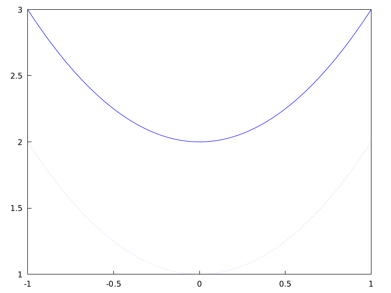

See also line_width.

Categories: Package draw ·

Graphic option: line_width ¶

Default value: 1

line_width is the width of plotted lines. Its value must be a positive number.

This option affects the following graphic objects:

• gr2d: points, polygon, rectangle, ellipse, vector, explicit, implicit, parametric and polar.
• gr3d: points and parametric.

Example:

(%i1) draw2d(explicit(x^2,x,-1,1), /* default width */
             line_width = 5.5,
             explicit(1 + x^2,x,-1,1),
             line_width = 10,
             explicit(2 + x^2,x,-1,1))$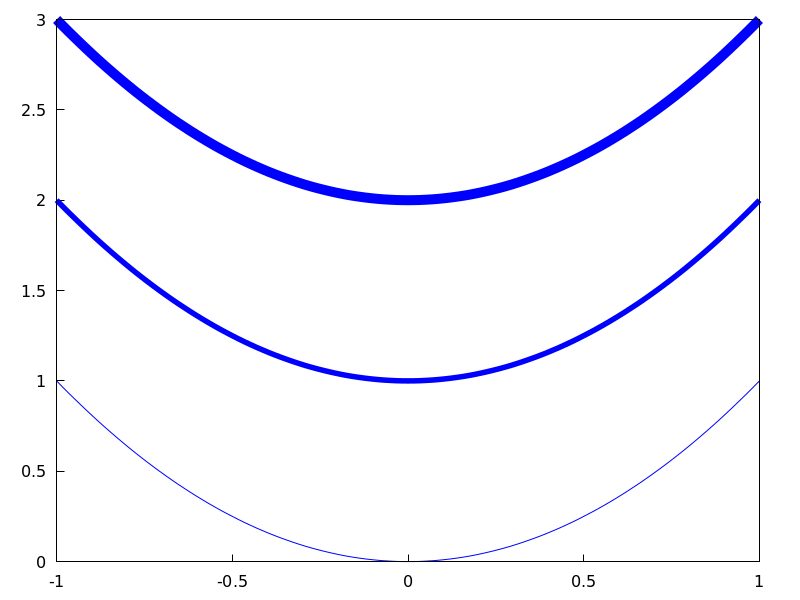

See also line_type.

Categories: Package draw ·

Graphic option: logcb ¶

Default value: false

If logcb is true, the tics in the colorbox will be drawn in the logarithmic scale.

When enhanced3d or colorbox is false, option logcb has no effect.

Since this is a global graphics option, its position in the scene description does not matter.

Example:

(%i1) draw3d (
        enhanced3d = true,
        color      = green,
        logcb = true,
        logz  = true,
        palette = [-15,24,-9],
        explicit(exp(x^2-y^2), x,-2,2,y,-2,2)) $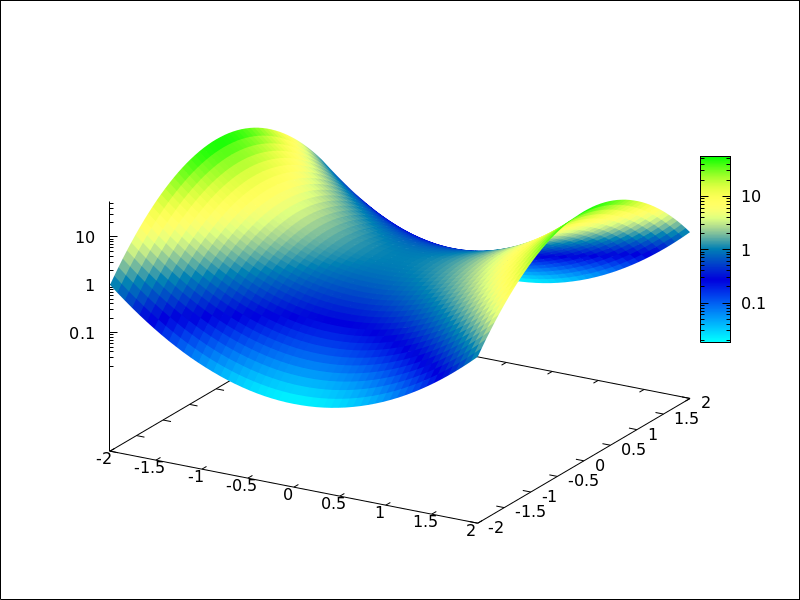

See also enhanced3d, colorbox and cbrange.

Categories: Package draw ·

Graphic option: logx ¶

Default value: false

If logx is true, the x axis will be drawn in the logarithmic scale.

Since this is a global graphics option, its position in the scene description does not matter, with the exception that it should be written before any 2D explicit object, so that draw can produce a better plot.

Example:

(%i1) draw2d(logx = true,
             explicit(log(x),x,0.01,5))$

See also logy, logx_secondary, logy_secondary, and logz.

Categories: Package draw ·

Graphic option: logx_secondary ¶

Default value: false

If logx_secondary is true, the secondary x axis will be drawn in the logarithmic scale.

This option is relevant only for 2d scenes.

Since this is a global graphics option, its position in the scene description does not matter.

Example:

(%i1) draw2d(
        grid = true,
        key="x^2, linear scale",
        color=red,
        explicit(x^2,x,1,100),
        xaxis_secondary = true,
        xtics_secondary = true,
        logx_secondary  = true,
        key = "x^2, logarithmic x scale",
        color = blue,
        explicit(x^2,x,1,100) )$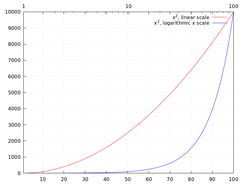

See also logx_draw, logy_draw, logy_secondary, and logz.

Categories: Package draw ·

Graphic option: logy ¶

Default value: false

If logy is true, the y axis will be drawn in the logarithmic scale.

Since this is a global graphics option, its position in the scene description does not matter.

Example:

(%i1) draw2d(logy = true,
             explicit(exp(x),x,0,5))$

See also logx_draw, logx_secondary, logy_secondary, and logz.

Categories: Package draw ·

Graphic option: logy_secondary ¶

Default value: false

If logy_secondary is true, the secondary y axis will be drawn in the logarithmic scale.

This option is relevant only for 2d scenes.

Since this is a global graphics option, its position in the scene description does not matter.

Example:

(%i1) draw2d(
        grid = true,
        key="x^2, linear scale",
        color=red,
        explicit(x^2,x,1,100),
        yaxis_secondary = true,
        ytics_secondary = true,
        logy_secondary  = true,
        key = "x^2, logarithmic y scale",
        color = blue,
        explicit(x^2,x,1,100) )$

See also logx_draw, logy_draw, logx_secondary, and logz.

Categories: Package draw ·

Graphic option: logz ¶

Default value: false

If logz is true, the z axis will be drawn in the logarithmic scale.

Since this is a global graphics option, its position in the scene description does not matter.

Example:

(%i1) draw3d(logz = true,
             explicit(exp(u^2+v^2),u,-2,2,v,-2,2))$

See also logx_draw and logy_draw.

Categories: Package draw ·

Graphic option: nticks ¶

Default value: 29

In 2d, nticks gives the initial number of points used by the adaptive plotting routine for explicit objects. It is also the number of points that will be shown in parametric and polar curves.

This option affects the following graphic objects:

• gr2d: ellipse, explicit, parametric and polar.
• gr3d: parametric.

See also adapt_depth

Example:

(%i1) draw2d(transparent = true,
             ellipse(0,0,4,2,0,180),
             nticks = 5,
             ellipse(0,0,4,2,180,180) )$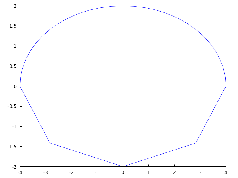

Categories: Package draw ·

Graphic option: palette ¶

Default value: color

palette indicates how to map gray levels onto color components. It works together with option enhanced3d in 3D graphics, who associates every point of a surfaces to a real number or gray level. It also works with gray images. With palette, levels are transformed into colors.

There are two ways for defining these transformations.

First, palette can be a vector of length three with components ranging from -36 to +36; each value is an index for a formula mapping the levels onto red, green and blue colors, respectively:

 0: 0               1: 0.5           2: 1
 3: x               4: x^2           5: x^3
 6: x^4             7: sqrt(x)       8: sqrt(sqrt(x))
 9: sin(90x)       10: cos(90x)     11: |x-0.5|
12: (2x-1)^2       13: sin(180x)    14: |cos(180x)|
15: sin(360x)      16: cos(360x)    17: |sin(360x)|
18: |cos(360x)|    19: |sin(720x)|  20: |cos(720x)|
21: 3x             22: 3x-1         23: 3x-2
24: |3x-1|         25: |3x-2|       26: (3x-1)/2 
27: (3x-2)/2       28: |(3x-1)/2|   29: |(3x-2)/2|
30: x/0.32-0.78125 31: 2*x-0.84     32: 4x;1;-2x+1.84;x/0.08-11.5
33: |2*x - 0.5|    34: 2*x          35: 2*x - 0.5
36: 2*x - 1

negative numbers mean negative colour component. palette = gray and palette = color are short cuts for palette = [3,3,3] and palette = [7,5,15], respectively.

Second, palette can be a user defined lookup table. In this case, the format for building a lookup table of length n is palette=[color_1, color_2, ..., color_n], where color_i is a well formed color (see option color) such that color_1 is assigned to the lowest gray level and color_n to the highest. The rest of colors are interpolated.

Since this is a global graphics option, its position in the scene description does not matter.

Examples:

It works together with option enhanced3d in 3D graphics.

(%i1) draw3d(
        enhanced3d = [z-x+2*y,x,y,z],
        palette = [32, -8, 17],
        explicit(20*exp(-x^2-y^2)-10,x,-3,3,y,-3,3))$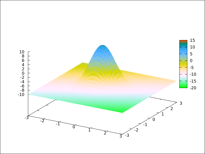

It also works with gray images.

(%i1) im: apply(
           'matrix,
            makelist(makelist(random(200),i,1,30),i,1,30))$
(%i2) /* palette = color, default */
      draw2d(image(im,0,0,30,30))$
(%i3) draw2d(palette = gray, image(im,0,0,30,30))$
(%i4) draw2d(palette = [15,20,-4],
             colorbox=false,
             image(im,0,0,30,30))$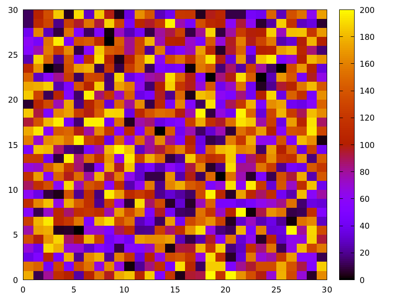

palette can be a user defined lookup table. In this example, low values of x are colored in red, and higher values in yellow.

(%i1) draw3d(
         palette = [red, blue, yellow],
         enhanced3d = x,
         explicit(x^2+y^2,x,-1,1,y,-1,1)) $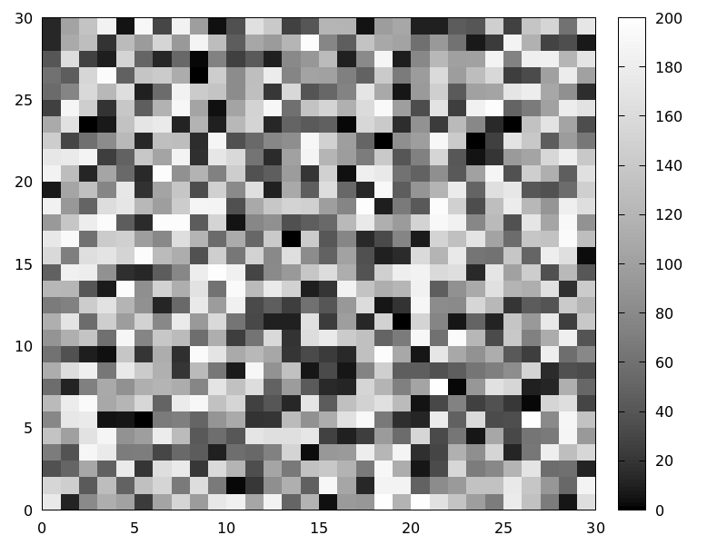

See also colorbox and enhanced3d.

Categories: Package draw ·

Graphic option: point_size ¶

Default value: 1

point_size sets the size for plotted points. It must be a non negative number.

This option has no effect when graphic option point_type is set to dot.

This option affects the following graphic objects:

• gr2d: points.
• gr3d: points.

Example:

(%i1) draw2d(points(makelist([random(20),random(50)],k,1,10)),
        point_size = 5,
        points(makelist(k,k,1,20),makelist(random(30),k,1,20)))$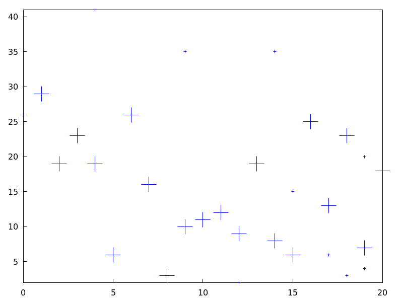

Categories: Package draw ·

Graphic option: point_type ¶

Default value: 1

point_type indicates how isolated points are displayed; the value of this option can be any integer index greater or equal than -1, or the name of a point style: $none (-1), dot (0), plus (1), multiply (2), asterisk (3), square (4), filled_square (5), circle (6), filled_circle (7), up_triangle (8), filled_up_triangle (9), down_triangle (10), filled_down_triangle (11), diamant (12) and filled_diamant (13).

This option affects the following graphic objects:

• gr2d: points.
• gr3d: points.

Example:

(%i1) draw2d(xrange = [0,10],
             yrange = [0,10],
             point_size = 3,
             point_type = diamant,
             points([[1,1],[5,1],[9,1]]),
             point_type = filled_down_triangle,
             points([[1,2],[5,2],[9,2]]),
             point_type = asterisk,
             points([[1,3],[5,3],[9,3]]),
             point_type = filled_diamant,
             points([[1,4],[5,4],[9,4]]),
             point_type = 5,
             points([[1,5],[5,5],[9,5]]),
             point_type = 6,
             points([[1,6],[5,6],[9,6]]),
             point_type = filled_circle,
             points([[1,7],[5,7],[9,7]]),
             point_type = 8,
             points([[1,8],[5,8],[9,8]]),
             point_type = filled_diamant,
             points([[1,9],[5,9],[9,9]]) )$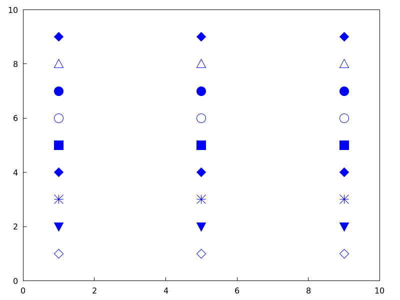

Categories: Package draw ·

Graphic option: points_joined ¶

Default value: false

When points_joined is true, points are joined by lines; when false, isolated points are drawn. A third possible value for this graphic option is impulses; in such case, vertical segments are drawn from points to the x-axis (2D) or to the xy-plane (3D).

This option affects the following graphic objects:

• gr2d: points.
• gr3d: points.

Example:

(%i1) draw2d(xrange        = [0,10],
             yrange        = [0,4],
             point_size    = 3,
             point_type    = up_triangle,
             color         = blue,
             points([[1,1],[5,1],[9,1]]),
             points_joined = true,
             point_type    = square,
             line_type     = dots,
             points([[1,2],[5,2],[9,2]]),
             point_type    = circle,
             color         = red,
             line_width    = 7,
             points([[1,3],[5,3],[9,3]]) )$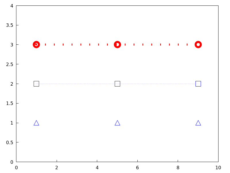

Categories: Package draw ·

Graphic option: proportional_axes ¶

Default value: none

When proportional_axes is equal to xy or xyz, the aspect ratio of the axis units will be set to 1:1 resulting in a 2D or 3D scene that will be drawn with axes proportional to their relative lengths.

Since this is a global graphics option, its position in the scene description does not matter.

This option works with Gnuplot version 4.2.6 or greater.

Examples:

Single 2D plot.

(%i1) draw2d(
        ellipse(0,0,1,1,0,360),
        transparent=true,
        color = blue,
        line_width = 4,
        ellipse(0,0,2,1/2,0,360),
        proportional_axes = 'xy) $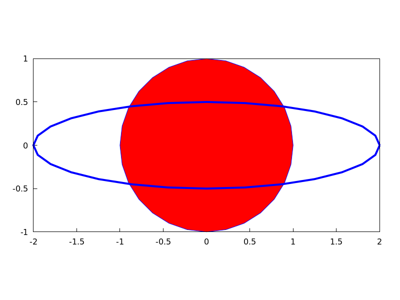

Multiplot.

(%i1) draw(
        terminal = wxt,
        gr2d(proportional_axes = 'xy,
             explicit(x^2,x,0,1)),
        gr2d(explicit(x^2,x,0,1),
             xrange = [0,1],
             yrange = [0,2],
             proportional_axes='xy),
        gr2d(explicit(x^2,x,0,1)))$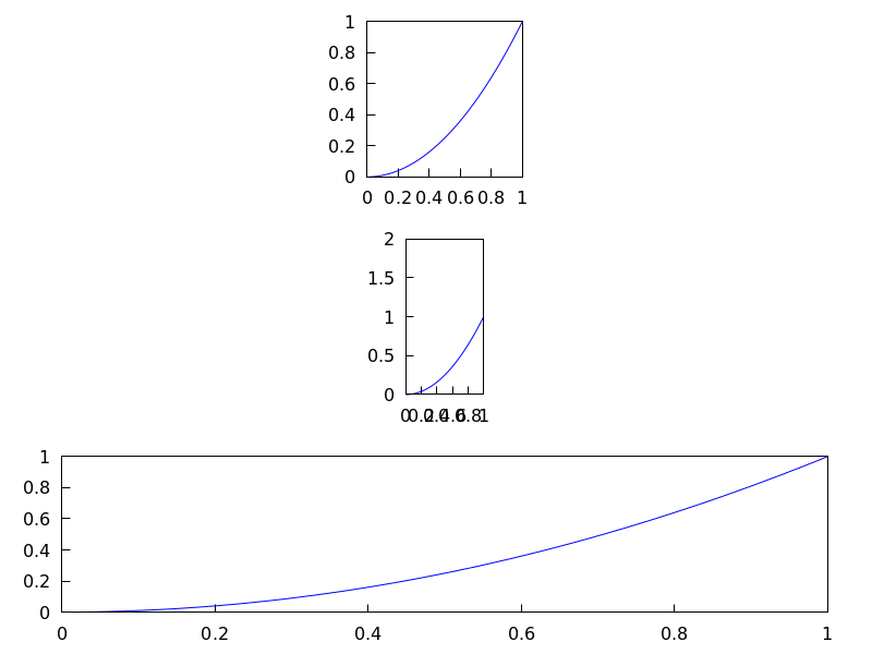

Categories: Package draw ·

Graphic option: surface_hide ¶

Default value: false

If surface_hide is true, hidden parts are not plotted in 3d surfaces.

Since this is a global graphics option, its position in the scene description does not matter.

Example:

(%i1) draw(columns=2,
           gr3d(explicit(exp(sin(x)+cos(x^2)),x,-3,3,y,-3,3)),
           gr3d(surface_hide = true,
                explicit(exp(sin(x)+cos(x^2)),x,-3,3,y,-3,3)) )$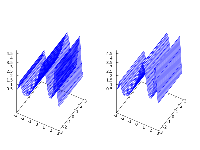

Categories: Package draw ·

Graphic option: terminal ¶

Default value: screen

Selects the terminal to be used by Gnuplot; possible values are: screen (default), png, pngcairo, jpg, gif, eps, eps_color, epslatex, epslatex_standalone, svg, canvas, dumb, dumb_file, pdf, pdfcairo, wxt, animated_gif, multipage_pdfcairo, multipage_pdf, multipage_eps, multipage_eps_color, and aquaterm.

Terminals screen, wxt, windows and aquaterm can be also defined as a list with two elements: the name of the terminal itself and a non negative integer number. In this form, multiple windows can be opened at the same time, each with its corresponding number. This feature does not work in Windows platforms.

Since this is a global graphics option, its position in the scene description does not matter. It can be also used as an argument of function draw.

N.B. pdfcairo requires Gnuplot 4.3 or newer. pdf requires Gnuplot to be compiled with the option --enable-pdf and libpdf must be installed. The pdf library is available from: http://www.pdflib.com/en/download/pdflib-family/pdflib-lite/

Examples:

(%i1) /* screen terminal (default) */
      draw2d(explicit(x^2,x,-1,1))$
(%i2) /* png file */
      draw2d(terminal  = 'png,
             explicit(x^2,x,-1,1))$
(%i3) /* jpg file */
      draw2d(terminal   = 'jpg,
             dimensions = [300,300],
             explicit(x^2,x,-1,1))$
(%i4) /* eps file */
      draw2d(file_name = "myfile",
             explicit(x^2,x,-1,1),
             terminal  = 'eps)$
(%i5) /* pdf file */
      draw2d(file_name = "mypdf",
             dimensions = 100*[12.0,8.0],
             explicit(x^2,x,-1,1),
             terminal  = 'pdf)$
(%i6) /* wxwidgets window */
      draw2d(explicit(x^2,x,-1,1),
             terminal  = 'wxt)$

Multiple windows.

(%i1) draw2d(explicit(x^5,x,-2,2), terminal=[screen, 3])$
(%i2) draw2d(explicit(x^2,x,-2,2), terminal=[screen, 0])$

An animated gif file.

(%i1) draw(
        delay     = 100,
        file_name = "zzz",
        terminal  = 'animated_gif,
        gr2d(explicit(x^2,x,-1,1)),
        gr2d(explicit(x^3,x,-1,1)),
        gr2d(explicit(x^4,x,-1,1)));
End of animation sequence
(%o1)          [gr2d(explicit), gr2d(explicit), gr2d(explicit)]

Option delay is only active in animated gif’s; it is ignored in any other case.

Multipage output in eps format.

(%i1) draw(
        file_name = "parabol",
        terminal  = multipage_eps,
        dimensions = 100*[10,10],
        gr2d(explicit(x^2,x,-1,1)),
        gr3d(explicit(x^2+y^2,x,-1,1,y,-1,1))) $

See also file_name, dimensions_draw and delay.

Categories: Package draw ·

Graphic option: title ¶

Default value: "" (empty string)

Option title, a string, is the main title for the scene. By default, no title is written.

Since this is a global graphics option, its position in the scene description does not matter.

Example:

(%i1) draw2d(explicit(exp(u),u,-2,2),
             title = "Exponential function")$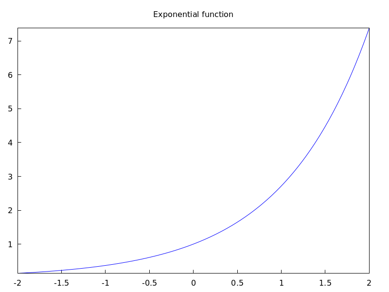

Categories: Package draw ·

Graphic option: transform ¶

Default value: none

If transform is none, the space is not transformed and graphic objects are drawn as defined. When a space transformation is desired, a list must be assigned to option transform. In case of a 2D scene, the list takes the form [f1(x,y), f2(x,y), x, y]. In case of a 3D scene, the list is of the form [f1(x,y,z), f2(x,y,z), f3(x,y,z), x, y, z].

The names of the variables defined in the lists may be different to those used in the definitions of the graphic objects.

Examples:

Rotation in 2D.

(%i1) th : %pi / 4$
(%i2) draw2d(
        color = "#e245f0",
        proportional_axes = 'xy,
        line_width = 8,
        triangle([3,2],[7,2],[5,5]),
        border     = false,
        fill_color = yellow,
        transform  = [cos(th)*x - sin(th)*y,
                      sin(th)*x + cos(th)*y, x, y],
        triangle([3,2],[7,2],[5,5]) )$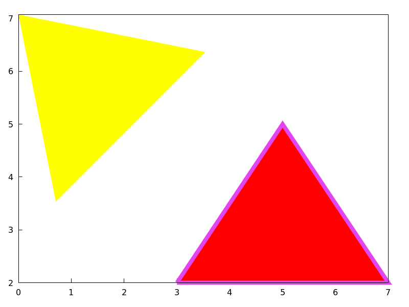

Translation in 3D.

(%i1) draw3d(
        color     = "#a02c00",
        explicit(20*exp(-x^2-y^2)-10,x,-3,3,y,-3,3),
        transform = [x+10,y+10,z+10,x,y,z],
        color     = blue,
        explicit(20*exp(-x^2-y^2)-10,x,-3,3,y,-3,3) )$

Categories: Package draw ·

Graphic option: transparent ¶

Default value: false

If transparent is false, interior regions of polygons are filled according to fill_color.

This option affects the following graphic objects:

• gr2d: polygon, rectangle and ellipse.

Example:

(%i1) draw2d(polygon([[3,2],[7,2],[5,5]]),
             transparent = true,
             color       = blue,
             polygon([[5,2],[9,2],[7,5]]) )$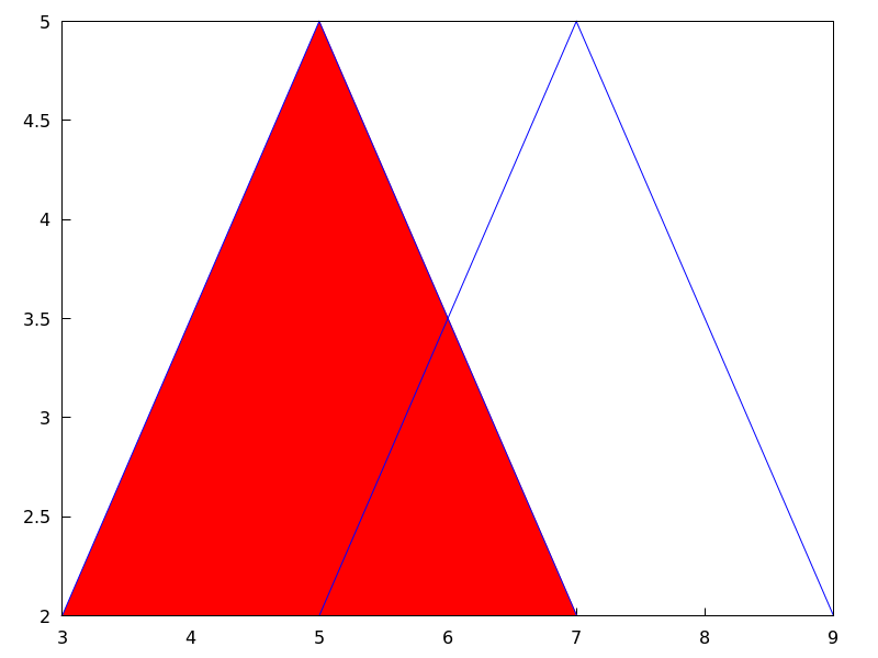

Categories: Package draw ·

Graphic option: unit_vectors ¶

Default value: false

If unit_vectors is true, vectors are plotted with module 1. This is useful for plotting vector fields. If unit_vectors is false, vectors are plotted with its original length.

This option is relevant only for vector objects.

Example:

(%i1) draw2d(xrange      = [-1,6],
             yrange      = [-1,6],
             head_length = 0.1,
             vector([0,0],[5,2]),
             unit_vectors = true,
             color        = red,
             vector([0,3],[5,2]))$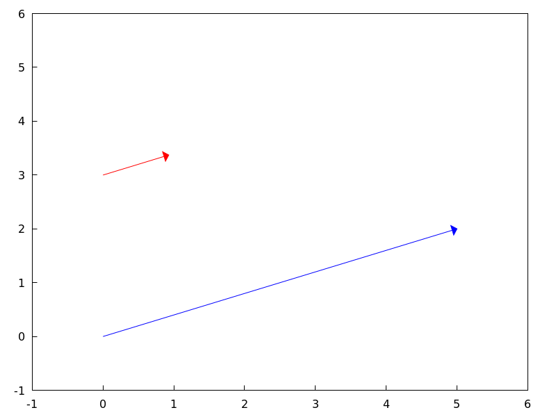

Categories: Package draw ·

Graphic option: user_preamble ¶

Default value: "" (empty string)

Expert Gnuplot users can make use of this option to fine tune Gnuplot’s behaviour by writing settings to be sent before the plot or splot command.

The value of this option must be a string or a list of strings (one per line).

Since this is a global graphics option, its position in the scene description does not matter.

Example:

Tell Gnuplot to draw axes and grid on top of graphics objects,

(%i1) draw2d(
        xaxis =true, xaxis_type=solid,
        yaxis =true, yaxis_type=solid,
        user_preamble="set grid front",
        region(x^2+y^2<1 ,x,-1.5,1.5,y,-1.5,1.5))$

Tell gnuplot to draw all contour lines in black

(%i1) draw3d(
          contour=both,
          surface_hide=true,enhanced3d=true,wired_surface=true,
          contour_levels=10,
          user_preamble="set for [i=1:8] linetype i dashtype i linecolor 0",
          explicit(sin(x)*cos(y),x,1,10,y,1,10)
      );

Categories: Package draw ·

Graphic option: view ¶

Default value: [60,30]

A pair of angles, measured in degrees, indicating the view direction in a 3D scene. The first angle is the vertical rotation around the x axis, in the range \([0, 360]\). The second one is the horizontal rotation around the z axis, in the range \([0, 360]\).

If option view is given the value map, the view direction is set to be perpendicular to the xy-plane.

Since this is a global graphics option, its position in the scene description does not matter.

Example:

(%i1) draw3d(view = [170, 50],
             enhanced3d = true,
             explicit(sin(x^2+y^2),x,-2,2,y,-2,2) )$

(%i2) draw3d(view = map,
             enhanced3d = true,
             explicit(sin(x^2+y^2),x,-2,2,y,-2,2) )$

Categories: Package draw ·

Graphic option: wired_surface ¶

Default value: false

Indicates whether 3D surfaces in enhanced3d mode show the grid joining the points or not.

Since this is a global graphics option, its position in the scene description does not matter.

Example:

(%i1) draw3d(
        enhanced3d    = [sin(x),x,y],
        wired_surface = true,
        explicit(x^2+y^2,x,-1,1,y,-1,1)) $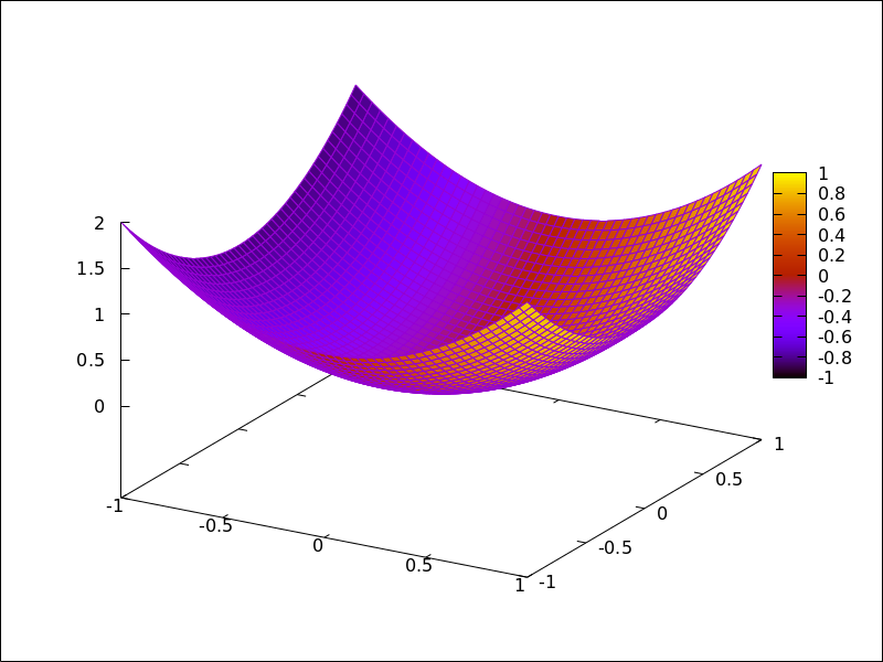

Categories: Package draw ·

Graphic option: x_voxel ¶

Default value: 10

x_voxel is the number of voxels in the x direction to be used by the marching cubes algorithm implemented by the 3d implicit object. It is also used by graphic object region.

Categories: Package draw ·

Graphic option: xaxis ¶

Default value: false

If xaxis is true, the x axis is drawn.

Since this is a global graphics option, its position in the scene description does not matter.

Example:

(%i1) draw2d(explicit(x^3,x,-1,1),
             xaxis       = true,
             xaxis_color = blue)$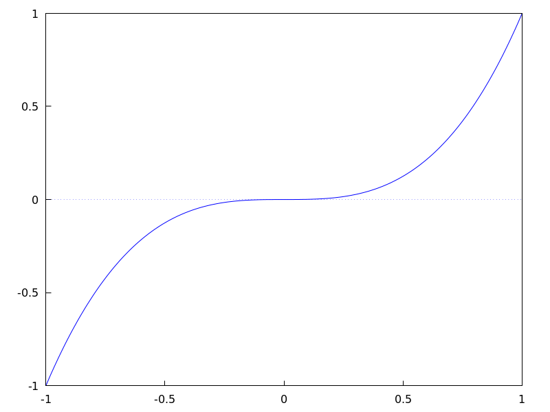

See also xaxis_width, xaxis_type and xaxis_color.

Categories: Package draw ·

Graphic option: xaxis_color ¶

Default value: "black"

xaxis_color specifies the color for the x axis. See color to know how colors are defined.

Since this is a global graphics option, its position in the scene description does not matter.

Example:

(%i1) draw2d(explicit(x^3,x,-1,1),
             xaxis       = true,
             xaxis_color = red)$

See also xaxis, xaxis_width and xaxis_type.

Categories: Package draw ·

Graphic option: xaxis_secondary ¶

Default value: false

If xaxis_secondary is true, function values can be plotted with respect to the second x axis, which will be drawn on top of the scene.

Note that this is a local graphics option which only affects to 2d plots.

Example:

(%i1) draw2d(
         key   = "Bottom x-axis",
         explicit(x+1,x,1,2),
         color = red,
         key   = "Above x-axis",
         xtics_secondary = true,
         xaxis_secondary = true,
         explicit(x^2,x,-1,1)) $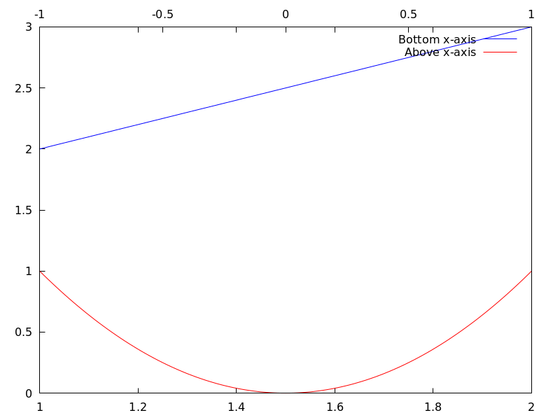

See also xrange_secondary, xtics_secondary, xtics_rotate_secondary, xtics_axis_secondary and xaxis_secondary.

Categories: Package draw ·

Graphic option: xaxis_type ¶

Default value: dots

xaxis_type indicates how the x axis is displayed; possible values are solid and dots

Since this is a global graphics option, its position in the scene description does not matter.

Example:

(%i1) draw2d(explicit(x^3,x,-1,1),
             xaxis       = true,
             xaxis_type  = solid)$

See also xaxis, xaxis_width and xaxis_color.

Categories: Package draw ·

Graphic option: xaxis_width ¶

Default value: 1

xaxis_width is the width of the x axis. Its value must be a positive number.

Since this is a global graphics option, its position in the scene description does not matter.

Example:

(%i1) draw2d(explicit(x^3,x,-1,1),
             xaxis       = true,
             xaxis_width = 3)$

See also xaxis, xaxis_type and xaxis_color.

Categories: Package draw ·

Graphic option: xlabel ¶

Default value: ""

Option xlabel, a string, is the label for the x axis. By default, the axis is labeled with string "x".

Since this is a global graphics option, its position in the scene description does not matter.

Example:

(%i1) draw2d(xlabel = "Time",
             explicit(exp(u),u,-2,2),
             ylabel = "Population")$

See also xlabel_secondary, ylabel, ylabel_secondary and zlabel_draw.

Categories: Package draw ·

Graphic option: xlabel_secondary ¶

Default value: "" (empty string)

Option xlabel_secondary, a string, is the label for the secondary x axis. By default, no label is written.

Since this is a global graphics option, its position in the scene description does not matter.

Example:

(%i1) draw2d(
         xaxis_secondary=true,yaxis_secondary=true,
         xtics_secondary=true,ytics_secondary=true,
         xlabel_secondary="t[s]",
         ylabel_secondary="U[V]",
         explicit(sin(t),t,0,10) )$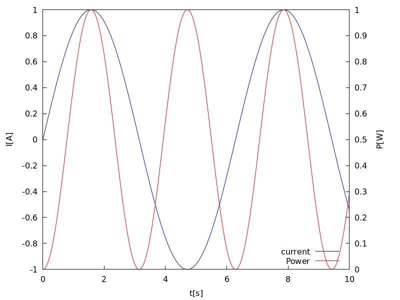

See also xlabel_draw, ylabel_draw, ylabel_secondary and zlabel_draw.

Categories: Package draw ·

Graphic option: xrange ¶

Default value: auto

If xrange is auto, the range for the x coordinate is computed automatically.

If the user wants a specific interval for x, it must be given as a Maxima list, as in xrange=[-2, 3].

Since this is a global graphics option, its position in the scene description does not matter.

Example:

(%i1) draw2d(xrange = [-3,5],
             explicit(x^2,x,-1,1))$

See also yrange and zrange.

Categories: Package draw ·

Graphic option: xrange_secondary ¶

Default value: auto

If xrange_secondary is auto, the range for the second x axis is computed automatically.

If the user wants a specific interval for the second x axis, it must be given as a Maxima list, as in xrange_secondary=[-2, 3].

Since this is a global graphics option, its position in the scene description does not matter.

See also xrange, yrange, zrange and yrange_secondary.

Categories: Package draw ·

Graphic option: xtics ¶

Default value: true

This graphic option controls the way tic marks are drawn on the x axis.

• When option xtics is bounded to symbol true, tic marks are drawn automatically.
• When option xtics is bounded to symbol false, tic marks are not drawn.
• When option xtics is bounded to a positive number, this is the distance between two consecutive tic marks.
• When option xtics is bounded to a list of length three of the form [start,incr,end], tic marks are plotted from start to end at intervals of length incr.
• When option xtics is bounded to a set of numbers of the form {n1, n2, ...}, tic marks are plotted at values n1, n2, ...
• When option xtics is bounded to a set of pairs of the form {["label1", n1], ["label2", n2], ...}, tic marks corresponding to values n1, n2, ... are labeled with "label1", "label2", ..., respectively.

Since this is a global graphics option, its position in the scene description does not matter.

Examples:

Disable tics.

(%i1) draw2d(xtics = 'false,
             explicit(x^3,x,-1,1)  )$

Tics every 1/4 units.

(%i1) draw2d(xtics = 1/4,
             explicit(x^3,x,-1,1)  )$

Tics from -3/4 to 3/4 in steps of 1/8.

(%i1) draw2d(xtics = [-3/4,1/8,3/4],
             explicit(x^3,x,-1,1)  )$

Tics at points -1/2, -1/4 and 3/4.

(%i1) draw2d(xtics = {-1/2,-1/4,3/4},
             explicit(x^3,x,-1,1)  )$

Labeled tics.

(%i1) draw2d(xtics = {["High",0.75],["Medium",0],["Low",-0.75]},
             explicit(x^3,x,-1,1)  )$

See also ytics_draw, and ztics_draw.

Categories: Package draw ·

Graphic option: xtics_axis ¶

Default value: false

If xtics_axis is true, tic marks and their labels are plotted just along the x axis, if it is false tics are plotted on the border.

Since this is a global graphics option, its position in the scene description does not matter.

Categories: Package draw ·

Graphic option: xtics_rotate ¶

Default value: false

If xtics_rotate is true, tic marks on the x axis are rotated 90 degrees.

Since this is a global graphics option, its position in the scene description does not matter.

Categories: Package draw ·

Graphic option: xtics_rotate_secondary ¶

Default value: false

If xtics_rotate_secondary is true, tic marks on the secondary x axis are rotated 90 degrees.

Since this is a global graphics option, its position in the scene description does not matter.

Categories: Package draw ·

Graphic option: xtics_secondary ¶

Default value: auto

This graphic option controls the way tic marks are drawn on the second x axis.

See xtics_draw for a complete description.

Categories: Package draw ·

Graphic option: xtics_secondary_axis ¶

Default value: false

If xtics_secondary_axis is true, tic marks and their labels are plotted just along the secondary x axis, if it is false tics are plotted on the border.

Since this is a global graphics option, its position in the scene description does not matter.

Categories: Package draw ·

Graphic option: xu_grid ¶

Default value: 30

xu_grid is the number of coordinates of the first variable (x in explicit and u in parametric 3d surfaces) to build the grid of sample points.

This option affects the following graphic objects:

• gr3d: explicit and parametric_surface.

Example:

(%i1) draw3d(xu_grid = 10,
             yv_grid = 50,
             explicit(x^2+y^2,x,-3,3,y,-3,3) )$

See also yv_grid.

Categories: Package draw ·

Graphic option: xy_file ¶

Default value: "" (empty string)

xy_file is the name of the file where the coordinates will be saved after clicking with the mouse button and hitting the ’x’ key. By default, no coordinates are saved.

Since this is a global graphics option, its position in the scene description does not matter.

Categories: Package draw ·

Graphic option: xyplane ¶

Default value: false

Allocates the xy-plane in 3D scenes. When xyplane is false, the xy-plane is placed automatically; when it is a real number, the xy-plane intersects the z-axis at this level. This option has no effect in 2D scenes.

Since this is a global graphics option, its position in the scene description does not matter.

Example:

(%i1) draw3d(xyplane = %e-2,
             explicit(x^2+y^2,x,-1,1,y,-1,1))$

Categories: Package draw ·

Graphic option: y_voxel ¶

Default value: 10

y_voxel is the number of voxels in the y direction to be used by the marching cubes algorithm implemented by the 3d implicit object. It is also used by graphic object region.

Categories: Package draw ·

Graphic option: yaxis ¶

Default value: false

If yaxis is true, the y axis is drawn.

Since this is a global graphics option, its position in the scene description does not matter.

Example:

(%i1) draw2d(explicit(x^3,x,-1,1),
             yaxis       = true,
             yaxis_color = blue)$

See also yaxis_width, yaxis_type and yaxis_color.

Categories: Package draw ·

Graphic option: yaxis_color ¶

Default value: "black"

yaxis_color specifies the color for the y axis. See color to know how colors are defined.

Since this is a global graphics option, its position in the scene description does not matter.

Example:

(%i1) draw2d(explicit(x^3,x,-1,1),
             yaxis       = true,
             yaxis_color = red)$

See also yaxis, yaxis_width and yaxis_type.

Categories: Package draw ·

Graphic option: yaxis_secondary ¶

Default value: false

If yaxis_secondary is true, function values can be plotted with respect to the second y axis, which will be drawn on the right side of the scene.

Note that this is a local graphics option which only affects to 2d plots.

Example:

(%i1) draw2d(
         explicit(sin(x),x,0,10),
         yaxis_secondary = true,
         ytics_secondary = true,
         color = blue,
         explicit(100*sin(x+0.1)+2,x,0,10));

See also yrange_secondary, ytics_secondary, ytics_rotate_secondary and ytics_axis_secondary

Categories: Package draw ·

Graphic option: yaxis_type ¶

Default value: dots

yaxis_type indicates how the y axis is displayed; possible values are solid and dots.

Since this is a global graphics option, its position in the scene description does not matter.

Example:

(%i1) draw2d(explicit(x^3,x,-1,1),
             yaxis       = true,
             yaxis_type  = solid)$

See also yaxis, yaxis_width and yaxis_color.

Categories: Package draw ·

Graphic option: yaxis_width ¶

Default value: 1

yaxis_width is the width of the y axis. Its value must be a positive number.

Since this is a global graphics option, its position in the scene description does not matter.

Example:

(%i1) draw2d(explicit(x^3,x,-1,1),
             yaxis       = true,
             yaxis_width = 3)$

See also yaxis, yaxis_type and yaxis_color.

Categories: Package draw ·

Graphic option: ylabel ¶

Default value: ""

Option ylabel, a string, is the label for the y axis. By default, the axis is labeled with string "y".

Since this is a global graphics option, its position in the scene description does not matter.

Example:

(%i1) draw2d(xlabel = "Time",
             ylabel = "Population",
             explicit(exp(u),u,-2,2) )$

See also xlabel_draw, xlabel_secondary, ylabel_secondary, and zlabel_draw.

Categories: Package draw ·

Graphic option: ylabel_secondary ¶

Default value: "" (empty string)

Option ylabel_secondary, a string, is the label for the secondary y axis. By default, no label is written.

Since this is a global graphics option, its position in the scene description does not matter.

Example:

(%i1) draw2d(
        key_pos=bottom_right,
        key="current",
        xlabel="t[s]",
        ylabel="I[A]",ylabel_secondary="P[W]",
        explicit(sin(t),t,0,10),
        yaxis_secondary=true,
        ytics_secondary=true,
        color=red,key="Power",
        explicit((sin(t))^2,t,0,10)
    )$

See also xlabel_draw, xlabel_secondary, ylabel_draw and zlabel_draw.

Categories: Package draw ·

Graphic option: yrange ¶

Default value: auto

If yrange is auto, the range for the y coordinate is computed automatically.

If the user wants a specific interval for y, it must be given as a Maxima list, as in yrange=[-2, 3].

Since this is a global graphics option, its position in the scene description does not matter.

Example:

(%i1) draw2d(yrange = [-2,3],
             explicit(x^2,x,-1,1),
             xrange = [-3,3])$

See also xrange, yrange_secondary and zrange.

Categories: Package draw ·

Graphic option: yrange_secondary ¶

Default value: auto

If yrange_secondary is auto, the range for the second y axis is computed automatically.

If the user wants a specific interval for the second y axis, it must be given as a Maxima list, as in yrange_secondary=[-2, 3].

Since this is a global graphics option, its position in the scene description does not matter.

Example:

(%i1) draw2d(
         explicit(sin(x),x,0,10),
         yaxis_secondary = true,
         ytics_secondary = true,
         yrange = [-3, 3],
         yrange_secondary = [-20, 20],
         color = blue,
         explicit(100*sin(x+0.1)+2,x,0,10)) $

See also xrange, yrange and zrange.

Categories: Package draw ·

Graphic option: ytics ¶

Default value: true

This graphic option controls the way tic marks are drawn on the y axis.

See xtics for a complete description.

Categories: Package draw ·

Graphic option: ytics_axis ¶

Default value: false

If ytics_axis is true, tic marks and their labels are plotted just along the y axis, if it is false tics are plotted on the border.

Since this is a global graphics option, its position in the scene description does not matter.

Categories: Package draw ·

Graphic option: ytics_rotate ¶

Default value: false

If ytics_rotate is true, tic marks on the y axis are rotated 90 degrees.

Since this is a global graphics option, its position in the scene description does not matter.

Categories: Package draw ·

Graphic option: ytics_rotate_secondary ¶

Default value: false

If ytics_rotate_secondary is true, tic marks on the secondary y axis are rotated 90 degrees.

Since this is a global graphics option, its position in the scene description does not matter.

Categories: Package draw ·

Graphic option: ytics_secondary ¶

Default value: auto

This graphic option controls the way tic marks are drawn on the second y axis.

See xtics for a complete description.

Categories: Package draw ·

Graphic option: ytics_secondary_axis ¶

Default value: false

If ytics_secondary_axis is true, tic marks and their labels are plotted just along the secondary y axis, if it is false tics are plotted on the border.

Since this is a global graphics option, its position in the scene description does not matter.

Categories: Package draw ·

Graphic option: yv_grid ¶

Default value: 30

yv_grid is the number of coordinates of the second variable (y in explicit and v in parametric 3d surfaces) to build the grid of sample points.

This option affects the following graphic objects:

• gr3d: explicit and parametric_surface.

Example:

(%i1) draw3d(xu_grid = 10,
             yv_grid = 50,
             explicit(x^2+y^2,x,-3,3,y,-3,3) )$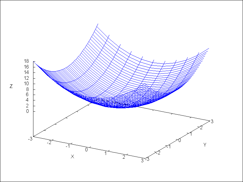

See also xu_grid.

Categories: Package draw ·

Graphic option: z_voxel ¶

Default value: 10

z_voxel is the number of voxels in the z direction to be used by the marching cubes algorithm implemented by the 3d implicit object.

Categories: Package draw ·

Graphic option: zaxis ¶

Default value: false

If zaxis is true, the z axis is drawn in 3D plots. This option has no effect in 2D scenes.

Since this is a global graphics option, its position in the scene description does not matter.

Example:

(%i1) draw3d(explicit(x^2+y^2,x,-1,1,y,-1,1),
             zaxis       = true,
             zaxis_type  = solid,
             zaxis_color = blue)$

See also zaxis_width, zaxis_type and zaxis_color.

Categories: Package draw ·

Graphic option: zaxis_color ¶

Default value: "black"

zaxis_color specifies the color for the z axis. See color to know how colors are defined. This option has no effect in 2D scenes.

Since this is a global graphics option, its position in the scene description does not matter.

Example:

(%i1) draw3d(explicit(x^2+y^2,x,-1,1,y,-1,1),
             zaxis       = true,
             zaxis_type  = solid,
             zaxis_color = red)$

See also zaxis, zaxis_width and zaxis_type.

Categories: Package draw ·

Graphic option: zaxis_type ¶

Default value: dots

zaxis_type indicates how the z axis is displayed; possible values are solid and dots. This option has no effect in 2D scenes.

Since this is a global graphics option, its position in the scene description does not matter.

Example:

(%i1) draw3d(explicit(x^2+y^2,x,-1,1,y,-1,1),
             zaxis       = true,
             zaxis_type  = solid)$

See also zaxis, zaxis_width and zaxis_color.

Categories: Package draw ·

Graphic option: zaxis_width ¶

Default value: 1

zaxis_width is the width of the z axis. Its value must be a positive number. This option has no effect in 2D scenes.

Since this is a global graphics option, its position in the scene description does not matter.

Example:

(%i1) draw3d(explicit(x^2+y^2,x,-1,1,y,-1,1),
             zaxis       = true,
             zaxis_type  = solid,
             zaxis_width = 3)$

See also zaxis, zaxis_type and zaxis_color.

Categories: Package draw ·

Graphic option: zlabel ¶

Default value: ""

Option zlabel, a string, is the label for the z axis. By default, the axis is labeled with string "z".

Since this is a global graphics option, its position in the scene description does not matter.

Example:

(%i1) draw3d(zlabel = "Z variable",
             ylabel = "Y variable",
             explicit(sin(x^2+y^2),x,-2,2,y,-2,2),
             xlabel = "X variable" )$

See also xlabel_draw, ylabel_draw, and zlabel_rotate.

Categories: Package draw ·

Graphic option: zlabel_rotate ¶

Default value: "auto"

This graphics option allows to choose if the z axis label of 3d plots is drawn horizontal (false), vertical (true) or if maxima automatically chooses an orientation based on the length of the label (auto).

Since this is a global graphics option, its position in the scene description does not matter.

Example:

(%i1) draw3d(
          explicit(sin(x)*sin(y),x,0,10,y,0,10),
          zlabel_rotate=false
      )$

See also zlabel_draw.

Categories: Package draw ·

Graphic option: zrange ¶

Default value: auto

If zrange is auto, the range for the z coordinate is computed automatically.

If the user wants a specific interval for z, it must be given as a Maxima list, as in zrange=[-2, 3].

Since this is a global graphics option, its position in the scene description does not matter.

Example:

(%i1) draw3d(yrange = [-3,3],
             zrange = [-2,5],
             explicit(x^2+y^2,x,-1,1,y,-1,1),
             xrange = [-3,3])$

See also xrange and yrange.

Categories: Package draw ·

Graphic option: ztics ¶

Default value: true

This graphic option controls the way tic marks are drawn on the z axis.

See xtics_draw for a complete description.

Categories: Package draw ·

Graphic option: ztics_axis ¶

Default value: false

If ztics_axis is true, tic marks and their labels are plotted just along the z axis, if it is false tics are plotted on the border.

Since this is a global graphics option, its position in the scene description does not matter.

Categories: Package draw ·

Graphic option: ztics_rotate ¶

Default value: false

If ztics_rotate is true, tic marks on the z axis are rotated 90 degrees.

Since this is a global graphics option, its position in the scene description does not matter.

Categories: Package draw ·

53.2.4 Graphics objects

Graphic object: bars ([x1,h1,w1], [x2,h2,w2, ...]) ¶

Draws vertical bars in 2D.

2D

bars ([x1,h1,w1], [x2,h2,w2, ...]) draws bars centered at values x1, x2, ... with heights h1, h2, ... and widths w1, w2, ...

This object is affected by the following graphic options: key, fill_color, fill_density and line_width.

Example:

(%i1) draw2d(
       key          = "Group A",
       fill_color   = blue,
       fill_density = 0.2,
       bars([0.8,5,0.4],[1.8,7,0.4],[2.8,-4,0.4]),
       key          = "Group B",
       fill_color   = red,
       fill_density = 0.6,
       line_width   = 4,
       bars([1.2,4,0.4],[2.2,-2,0.4],[3.2,5,0.4]),
       xaxis = true);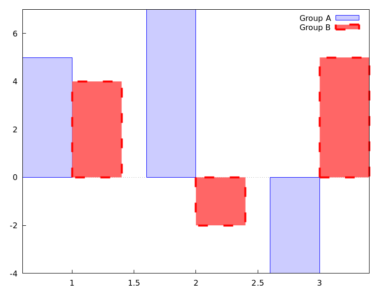

Categories: Package draw ·

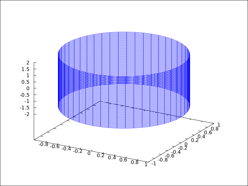
Graphic object: cylindrical (radius, z, minz, maxz, azi, minazi, maxazi) ¶

Draws 3D functions defined in cylindrical coordinates.

3D

cylindrical(radius, z, minz, maxz, azi, minazi, maxazi) plots the function radius(z, azi) defined in cylindrical coordinates, with variable z taking values from minz to maxz and azimuth azi taking values from minazi to maxazi.

This object is affected by the following graphic options: xu_grid, yv_grid, line_type, key, wired_surface, enhanced3d and color

Example:

(%i1) draw3d(cylindrical(1,z,-2,2,az,0,2*%pi))$

Categories: Package draw ·

Graphic object: elevation_grid (mat,x0,y0,width,height) ¶

Draws matrix mat in 3D space. z values are taken from mat, the abscissas range from x0 to x0 + width and ordinates from y0 to y0 + height. Element \(a(1,1)\) is projected on point \((x0,y0+height)\), \(a(1,n)\) on \((x0+width,y0+height)\), \(a(m,1)\) on \((x0,y0)\), and \(a(m,n)\) on \((x0+width,y0)\).

This object is affected by the following graphic options: line_type,, line_width key, wired_surface, enhanced3d and color

In older versions of Maxima, elevation_grid was called mesh. See also mesh.

Example:

(%i1) m: apply(
            matrix,
            makelist(makelist(random(10.0),k,1,30),i,1,20)) $
(%i2) draw3d(
         color = blue,
         elevation_grid(m,0,0,3,2),
         xlabel = "x",
         ylabel = "y",
         surface_hide = true);

Categories: Package draw ·

Graphic object: ellipse (xc, yc, a, b, ang1, ang2) ¶

Draws ellipses and circles in 2D.

2D

ellipse (xc, yc, a, b, ang1, ang2) plots an ellipse centered at [xc, yc] with horizontal and vertical semi axis a and b, respectively, starting at angle ang1 with an amplitude equal to angle ang2.

This object is affected by the following graphic options: nticks, transparent, fill_color, fill_density, border, line_width, line_type, key and color

Example:

(%i1) draw2d(transparent = false,
             fill_color  = red,
             color       = gray30,
             transparent = false,
             line_width  = 5,
             ellipse(0,6,3,2,270,-270),
             /* center (x,y), a, b, start & end in degrees */
             transparent = true,
             color       = blue,
             line_width  = 3,
             ellipse(2.5,6,2,3,30,-90),
             xrange      = [-3,6],
             yrange      = [2,9] )$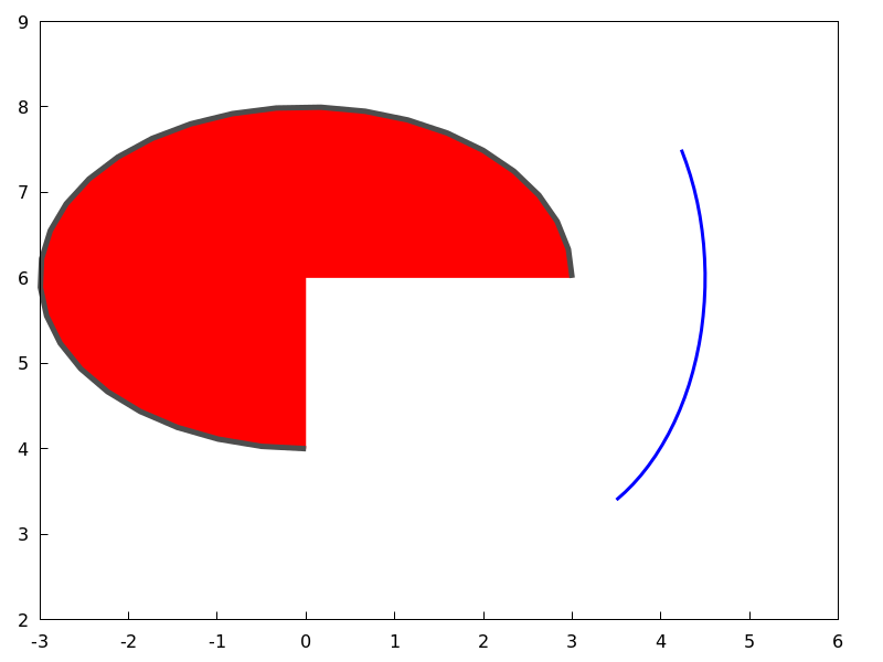

Categories: Package draw ·

Graphic object: errors ([x1, x2, …], [y1, y2, …]) ¶

Draws points with error bars, horizontally, vertically or both, depending on the value of option error_type.

2D

If error_type = x, arguments to errors must be of the form [x, y, xdelta] or [x, y, xlow, xhigh]. If error_type = y, arguments must be of the form [x, y, ydelta] or [x, y, ylow, yhigh]. If error_type = xy or error_type = boxes, arguments to errors must be of the form [x, y, xdelta, ydelta] or [x, y, xlow, xhigh, ylow, yhigh].

See also error_type.

This object is affected by the following graphic options: error_type, points_joined, line_width, key, line_type, color fill_density, xaxis_secondary and yaxis_secondary.

Option fill_density is only relevant when error_type=boxes.

Examples:

Horizontal error bars.

(%i1) draw2d(
        error_type = 'y,
        errors([[1,2,1], [3,5,3], [10,3,1], [17,6,2]]))$

Vertical and horizontal error bars.

(%i1) draw2d(
        error_type = 'xy,
        points_joined = true,
        color = blue,
        errors([[1,2,1,2], [3,5,2,1], [10,3,1,1], [17,6,1/2,2]])); 

Categories: Package draw ·

Graphic object: explicit
    explicit (expr,var,minval,maxval)
    explicit (fcn,var,minval,maxval)
    explicit (expr,var1,minval1,maxval1,var2,minval2,maxval2)
    explicit (fcn,var1,minval1,maxval1,var2,minval2,maxval2) ¶

Draws explicit functions in 2D and 3D.

2D

explicit(fcn,var,minval,maxval) plots explicit function fcn, with variable var taking values from minval to maxval.

This object is affected by the following graphic options: nticks, adapt_depth, draw_realpart, line_width, line_type, key, filled_func, fill_color, fill_density, and color

Example:

(%i1) draw2d(line_width = 3,
             color      = blue,
             explicit(x^2,x,-3,3) )$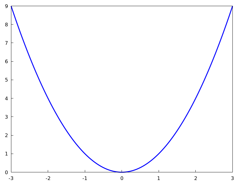

(%i2) draw2d(fill_color  = brown,
             filled_func = true,
             explicit(x^2,x,-3,3) )$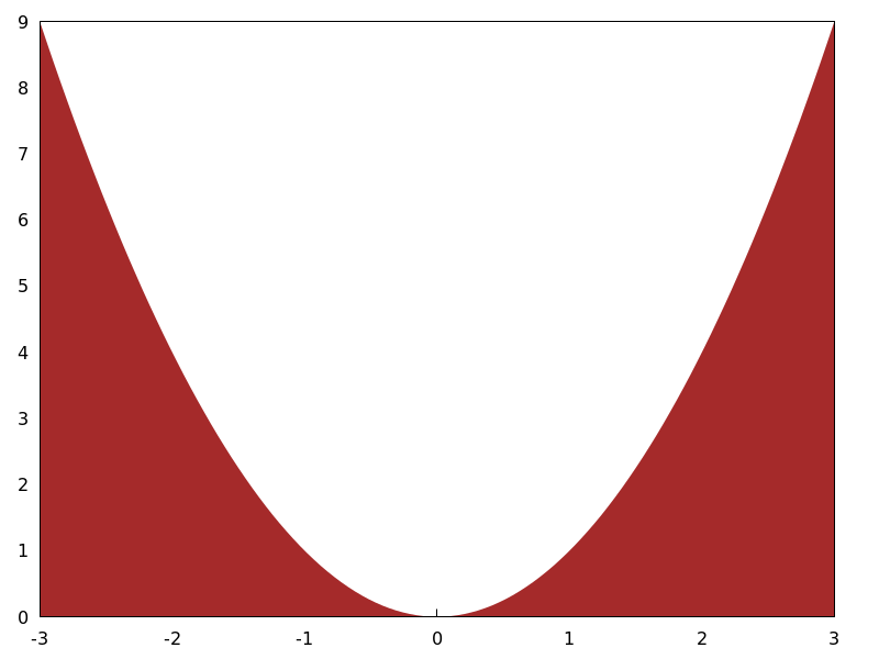

3D

explicit(fcn, var1, minval1, maxval1, var2, minval2, maxval2) plots the explicit function fcn, with variable var1 taking values from minval1 to maxval1 and variable var2 taking values from minval2 to maxval2.

This object is affected by the following graphic options: draw_realpart, xu_grid, yv_grid, line_type, line_width, key, wired_surface, enhanced3d and color.

Example:

(%i1) draw3d(key   = "Gauss",
             color = "#a02c00",
             explicit(20*exp(-x^2-y^2)-10,x,-3,3,y,-3,3),
             yv_grid     = 10,
             color = blue,
             key   = "Plane",
             explicit(x+y,x,-5,5,y,-5,5),
             surface_hide = true)$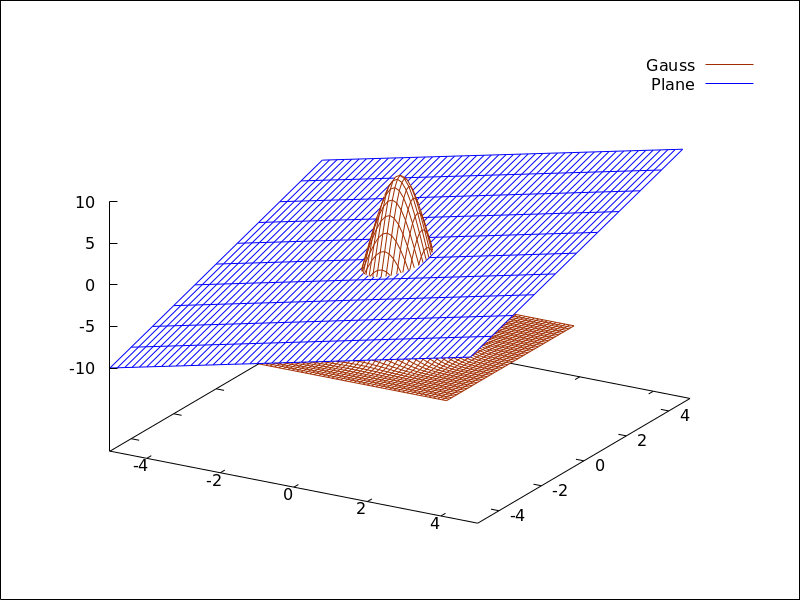

See also filled_func for filled functions.

Categories: Package draw ·

Graphic object: image (im,x0,y0,width,height) ¶

Renders images in 2D.

2D

image (im,x0,y0,width,height) plots image im in the rectangular region from vertex (x0,y0) to (x0+width,y0+height) on the real plane. Argument im must be a matrix of real numbers, a matrix of vectors of length three or a picture object.

If im is a matrix of real numbers or a levels picture object, pixel values are interpreted according to graphic option palette, which is a vector of length three with components ranging from -36 to +36; each value is an index for a formula mapping the levels onto red, green and blue colors, respectively:

 0: 0               1: 0.5           2: 1
 3: x               4: x^2           5: x^3
 6: x^4             7: sqrt(x)       8: sqrt(sqrt(x))
 9: sin(90x)       10: cos(90x)     11: |x-0.5|
12: (2x-1)^2       13: sin(180x)    14: |cos(180x)|
15: sin(360x)      16: cos(360x)    17: |sin(360x)|
18: |cos(360x)|    19: |sin(720x)|  20: |cos(720x)|
21: 3x             22: 3x-1         23: 3x-2
24: |3x-1|         25: |3x-2|       26: (3x-1)/2
27: (3x-2)/2       28: |(3x-1)/2|   29: |(3x-2)/2|
30: x/0.32-0.78125                  31: 2*x-0.84
32: 4x;1;-2x+1.84;x/0.08-11.5
33: |2*x - 0.5|    34: 2*x          35: 2*x - 0.5
36: 2*x - 1

negative numbers mean negative colour component.

palette = gray and palette = color are short cuts for palette = [3,3,3] and palette = [7,5,15], respectively.

If im is a matrix of vectors of length three or an rgb picture object, they are interpreted as red, green and blue color components.

Examples:

If im is a matrix of real numbers, pixel values are interpreted according to graphic option palette.

(%i1) im: apply(
           'matrix,
            makelist(makelist(random(200),i,1,30),i,1,30))$
(%i2) /* palette = color, default */
      draw2d(image(im,0,0,30,30))$

(%i3) draw2d(palette = gray, image(im,0,0,30,30))$

(%i4) draw2d(palette = [15,20,-4],
             colorbox=false,
             image(im,0,0,30,30))$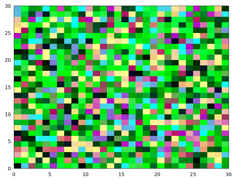

See also colorbox.

If im is a matrix of vectors of length three, they are interpreted as red, green and blue color components.

(%i1) im: apply(
            'matrix,
             makelist(
               makelist([random(300),
                         random(300),
                         random(300)],i,1,30),i,1,30))$
(%i2) draw2d(image(im,0,0,30,30))$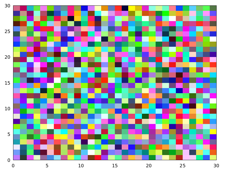

Package draw automatically loads package picture. In this example, a level picture object is built by hand and then rendered.

(%i1) im: make_level_picture([45,87,2,134,204,16],3,2);
(%o1)       picture(level, 3, 2, {Array:  #(45 87 2 134 204 16)})
(%i2) /* default color palette */
      draw2d(image(im,0,0,30,30))$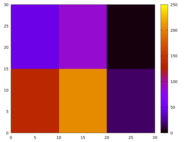

(%i3) /* gray palette */
      draw2d(palette = gray,
             image(im,0,0,30,30))$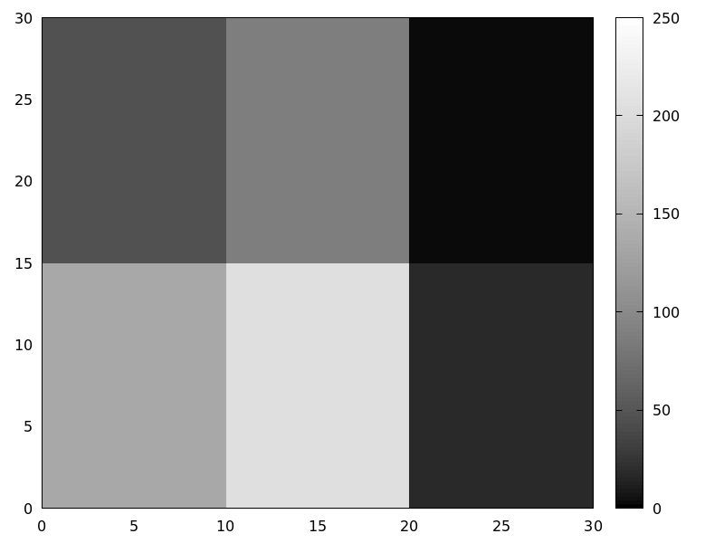

An xpm file is read and then rendered.

(%i1) im: read_xpm("myfile.xpm")$
(%i2) draw2d(image(im,0,0,10,7))$

See also make_level_picture, make_rgb_picture and read_xpm.

http://www.telefonica.net/web2/biomates/maxima/gpdraw/image
contains more elaborated examples.

Categories: Package draw ·

Graphic object: implicit
    implicit (fcn,x,xmin,xmax,y,ymin,ymax)
    implicit (fcn,x,xmin,xmax,y,ymin,ymax,z,zmin,zmax) ¶

Draws implicit functions in 2D and 3D.

2D

implicit(fcn,x,xmin,xmax,y,ymin,ymax) plots the implicit function defined by fcn, with variable x taking values from xmin to xmax, and variable y taking values from ymin to ymax.

This object is affected by the following graphic options: ip_grid, ip_grid_in, line_width, line_type, key and color.

Example:

(%i1) draw2d(grid      = true,
             line_type = solid,
             key       = "y^2=x^3-2*x+1",
             implicit(y^2=x^3-2*x+1, x, -4,4, y, -4,4),
             line_type = dots,
             key       = "x^3+y^3 = 3*x*y^2-x-1",
             implicit(x^3+y^3 = 3*x*y^2-x-1, x,-4,4, y,-4,4),
             title     = "Two implicit functions" )$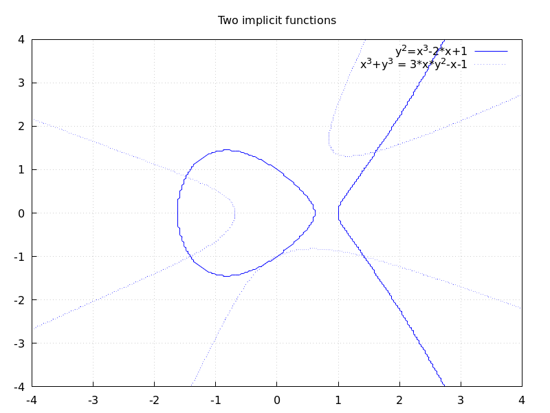

3D

implicit (fcn,x,xmin,xmax, y,ymin,ymax, z,zmin,zmax) plots the implicit surface defined by fcn, with variable x taking values from xmin to xmax, variable y taking values from ymin to ymax and variable z taking values from zmin to zmax. This object implements the marching cubes algorithm.

This object is affected by the following graphic options: x_voxel, y_voxel, z_voxel, line_width, line_type, key, wired_surface, enhanced3d and color.

Example:

(%i1) draw3d(
        color=blue,
        implicit((x^2+y^2+z^2-1)*(x^2+(y-1.5)^2+z^2-0.5)=0.015,
                 x,-1,1,y,-1.2,2.3,z,-1,1),
        surface_hide=true);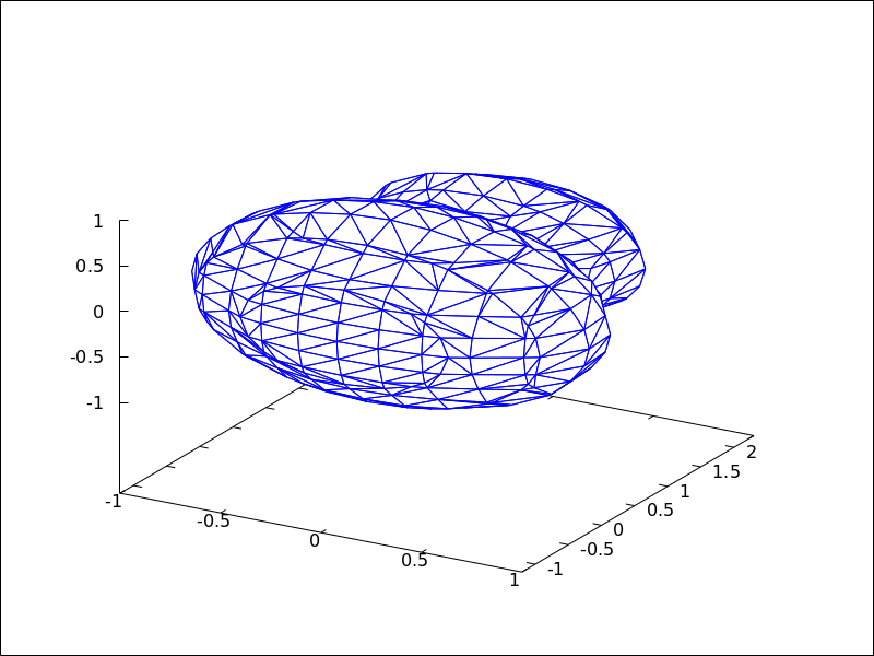

Categories: Package draw ·

Graphic object: label
    label ([string,x,y],...)
    label ([string,x,y,z],...) ¶

Writes labels in 2D and 3D.

Colored labels work only with Gnuplot 4.3 and up.

This object is affected by the following graphic options: label_alignment, label_orientation and color.

2D

label([string,x,y]) writes the string at point [x,y].

Example:

(%i1) draw2d(yrange = [0.1,1.4],
             color = red,
             label(["Label in red",0,0.3]),
             color = "#0000ff",
             label(["Label in blue",0,0.6]),
             color = light_blue,
             label(["Label in light-blue",0,0.9],
                   ["Another light-blue",0,1.2])  )$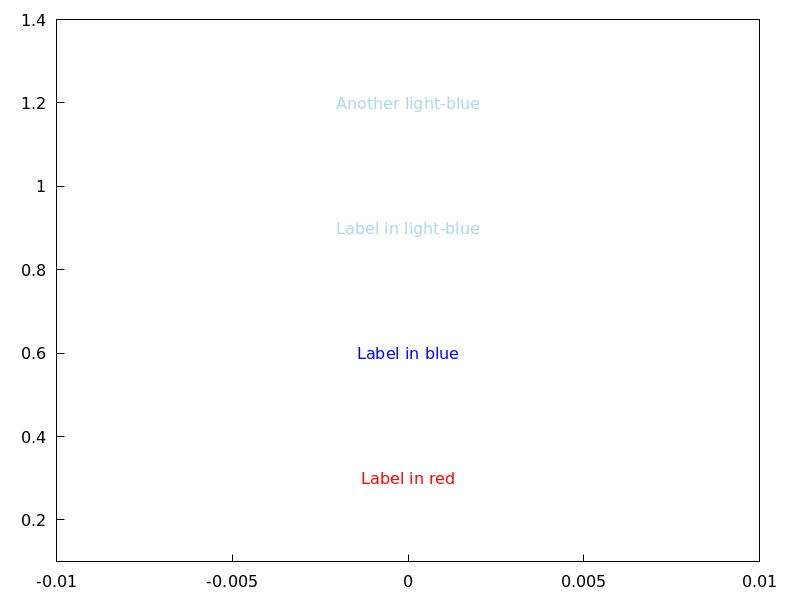

3D

label([string,x,y,z]) writes the string at point [x,y,z].

Example:

(%i1) draw3d(explicit(exp(sin(x)+cos(x^2)),x,-3,3,y,-3,3),
             color = red,
             label(["UP 1",-2,0,3], ["UP 2",1.5,0,4]),
             color = blue,
             label(["DOWN 1",2,0,-3]) )$

Categories: Package draw ·

Graphic object: mesh (row_1,row_2,...) ¶

Draws a quadrangular mesh in 3D.

3D

Argument row_i is a list of n 3D points of the form [[x_i1,y_i1,z_i1], ...,[x_in,y_in,z_in]], and all rows are of equal length. All these points define an arbitrary surface in 3D and in some sense it’s a generalization of the elevation_grid object.

This object is affected by the following graphic options: line_type, line_width, color, key, wired_surface, enhanced3d and transform.

Examples:

A simple example.

(%i1) draw3d( 
         mesh([[1,1,3],   [7,3,1],[12,-2,4],[15,0,5]],
              [[2,7,8],   [4,3,1],[10,5,8], [12,7,1]],
              [[-2,11,10],[6,9,5],[6,15,1], [20,15,2]])) $

Plotting a triangle in 3D.

(%i1) draw3d(
        line_width = 2,
        mesh([[1,0,0],[0,1,0]],
             [[0,0,1],[0,0,1]])) $

Two quadrilaterals.

(%i1) draw3d(
        surface_hide = true,
        line_width   = 3,
        color = red,
        mesh([[0,0,0], [0,1,0]],
             [[2,0,2], [2,2,2]]),
        color = blue,
        mesh([[0,0,2], [0,1,2]],
             [[2,0,4], [2,2,4]])) $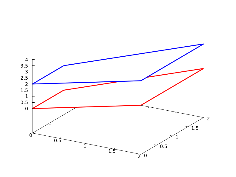

Categories: Package draw ·

Graphic object: parametric
    parametric (xfun,yfun,par,parmin,parmax)
    parametric (xfun,yfun,zfun,par,parmin,parmax) ¶

Draws parametric functions in 2D and 3D.

This object is affected by the following graphic options: nticks, line_width, line_type, key, color and enhanced3d.

2D

The command parametric(xfun, yfun, par, parmin, parmax) plots the parametric function [xfun, yfun], with parameter par taking values from parmin to parmax.

Example:

(%i1) draw2d(explicit(exp(x),x,-1,3),
             color = red,
             key   = "This is the parametric one!!",
             parametric(2*cos(rrr),rrr^2,rrr,0,2*%pi))$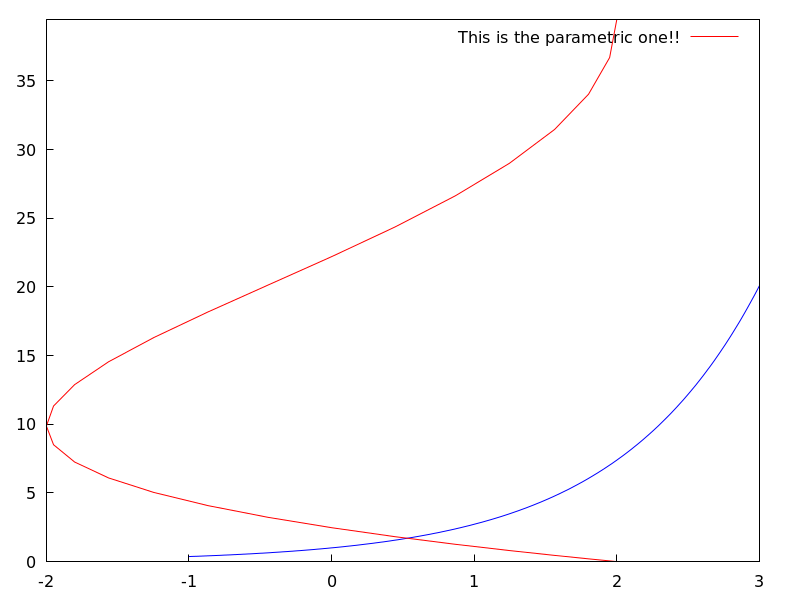

3D

parametric(xfun, yfun, zfun, par, parmin, parmax) plots the parametric curve [xfun, yfun, zfun], with parameter par taking values from parmin to parmax.

Example:

(%i1) draw3d(explicit(exp(sin(x)+cos(x^2)),x,-3,3,y,-3,3),
             color = royalblue,
             parametric(cos(5*u)^2,sin(7*u),u-2,u,0,2),
             color      = turquoise,
             line_width = 2,
             parametric(t^2,sin(t),2+t,t,0,2),
             surface_hide = true,
             title = "Surface & curves" )$

Categories: Package draw ·

Graphic object: parametric_surface (xfun, yfun, zfun, par1, par1min, par1max, par2, par2min, par2max) ¶

Draws parametric surfaces in 3D.

3D

The command parametric_surface(xfun, yfun, zfun, par1, par1min, par1max, par2, par2min, par2max) plots the parametric surface [xfun, yfun, zfun], with parameter par1 taking values from par1min to par1max and parameter par2 taking values from par2min to par2max.

This object is affected by the following graphic options: draw_realpart, xu_grid, yv_grid, line_type, line_width, key, wired_surface, enhanced3d and color.

Example:

(%i1) draw3d(title          = "Sea shell",
             xu_grid        = 100,
             yv_grid        = 25,
             view           = [100,20],
             surface_hide   = true,
             parametric_surface(0.5*u*cos(u)*(cos(v)+1),
                           0.5*u*sin(u)*(cos(v)+1),
                           u*sin(v) - ((u+3)/8*%pi)^2 - 20,
                           u, 0, 13*%pi, v, -%pi, %pi) )$

Categories: Package draw ·

Graphic object: points
    points ([[x1,y1], [x2,y2],...])
    points ([x1,x2,...], [y1,y2,...])
    points ([y1,y2,...])
    points ([[x1,y1,z1], [x2,y2,z2],...])
    points ([x1,x2,...], [y1,y2,...], [z1,z2,...])
    points (matrix)
    points (1d_y_array)
    points (1d_x_array, 1d_y_array)
    points (1d_x_array, 1d_y_array, 1d_z_array)
    points (2d_xy_array)
    points (2d_xyz_array) ¶

Draws points in 2D and 3D.

This object is affected by the following graphic options: point_size, point_type, points_joined, line_width, key, line_type and color. In 3D mode, it is also affected by enhanced3d

2D

points ([[x1,y1], [x2,y2],...]) or points ([x1,x2,...], [y1,y2,...]) plots points [x1,y1], [x2,y2], etc. If abscissas are not given, they are set to consecutive positive integers, so that points ([y1,y2,...]) draws points [1,y1], [2,y2], etc. If matrix is a two-column or two-row matrix, points (matrix) draws the associated points. If matrix is an one-column or one-row matrix, abscissas are assigned automatically.

If 1d_y_array is a 1D lisp array of numbers, points (1d_y_array) plots them setting abscissas to consecutive positive integers. points (1d_x_array, 1d_y_array) plots points with their coordinates taken from the two arrays passed as arguments. If 2d_xy_array is a 2D array with two columns, or with two rows, points (2d_xy_array) plots the corresponding points on the plane.

Examples:

Two types of arguments for points, a list of pairs and two lists of separate coordinates.

(%i1) draw2d(
        key = "Small points",
        points(makelist([random(20),random(50)],k,1,10)),
        point_type    = circle,
        point_size    = 3,
        points_joined = true,
        key           = "Great points",
        points(makelist(k,k,1,20),makelist(random(30),k,1,20)),
        point_type    = filled_down_triangle,
        key           = "Automatic abscissas",
        color         = red,
        points([2,12,8]))$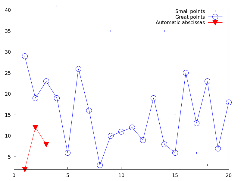

Drawing impulses.

(%i1) draw2d(
        points_joined = impulses,
        line_width    = 2,
        color         = red,
        points(makelist([random(20),random(50)],k,1,10)))$

Array with ordinates.

(%i1) a: make_array (flonum, 100) $
(%i2) for i:0 thru 99 do a[i]: random(1.0) $
(%i3) draw2d(points(a)) $

Two arrays with separate coordinates.

(%i1) x: make_array (flonum, 100) $
(%i2) y: make_array (fixnum, 100) $
(%i3) for i:0 thru 99 do (
        x[i]: float(i/100),
        y[i]: random(10) ) $
(%i4) draw2d(points(x, y)) $

A two-column 2D array.

(%i1) xy: make_array(flonum, 100, 2) $
(%i2) for i:0 thru 99 do (
        xy[i, 0]: float(i/100),
        xy[i, 1]: random(10) ) $
(%i3) draw2d(points(xy)) $

Drawing an array filled with function read_array.

(%i1) a: make_array(flonum,100) $
(%i2) read_array (file_search ("pidigits.data"), a) $
(%i3) draw2d(points(a)) $

3D

points([[x1, y1, z1], [x2, y2, z2], ...]) or points([x1, x2, ...], [y1, y2, ...], [z1, z2,...]) plots points [x1, y1, z1], [x2, y2, z2], etc. If matrix is a three-column or three-row matrix, points (matrix) draws the associated points.

When arguments are lisp arrays, points (1d_x_array, 1d_y_array, 1d_z_array) takes coordinates from the three 1D arrays. If 2d_xyz_array is a 2D array with three columns, or with three rows, points (2d_xyz_array) plots the corresponding points.

Examples:

One tridimensional sample,

(%i1) load ("numericalio")$
(%i2) s2 : read_matrix (file_search ("wind.data"))$
(%i3) draw3d(title = "Daily average wind speeds",
             point_size = 2,
             points(args(submatrix (s2, 4, 5))) )$

Two tridimensional samples,

(%i1) load ("numericalio")$
(%i2) s2 : read_matrix (file_search ("wind.data"))$
(%i3) draw3d(
         title = "Daily average wind speeds. Two data sets",
         point_size = 2,
         key        = "Sample from stations 1, 2 and 3",
         points(args(submatrix (s2, 4, 5))),
         point_type = 4,
         key        = "Sample from stations 1, 4 and 5",
         points(args(submatrix (s2, 2, 3))) )$

Unidimensional arrays,

(%i1) x: make_array (fixnum, 10) $
(%i2) y: make_array (fixnum, 10) $
(%i3) z: make_array (fixnum, 10) $
(%i4) for i:0 thru 9 do (
        x[i]: random(10),
        y[i]: random(10),
        z[i]: random(10) ) $
(%i5) draw3d(points(x,y,z)) $

Bidimensional colored array,

(%i1) xyz: make_array(fixnum, 10, 3) $
(%i2) for i:0 thru 9 do (
        xyz[i, 0]: random(10),
        xyz[i, 1]: random(10),
        xyz[i, 2]: random(10) ) $
(%i3) draw3d(
         enhanced3d = true,
         points_joined = true,
         points(xyz)) $

Color numbers explicitly specified by the user.

(%i1) pts: makelist([t,t^2,cos(t)], t, 0, 15)$
(%i2) col_num: makelist(k, k, 1, length(pts))$
(%i3) draw3d(
        enhanced3d = ['part(col_num,k),k],
        point_size = 3,
        point_type = filled_circle,
        points(pts))$

Categories: Package draw ·

Graphic object: polar (radius,ang,minang,maxang) ¶

Draws 2D functions defined in polar coordinates.

2D

polar (radius,ang,minang,maxang) plots function radius(ang) defined in polar coordinates, with variable ang taking values from minang to maxang.

This object is affected by the following graphic options: nticks, line_width, line_type, key and color.

Example:

(%i1) draw2d(user_preamble = "set grid polar",
             nticks        = 200,
             xrange        = [-5,5],
             yrange        = [-5,5],
             color         = blue,
             line_width    = 3,
             title         = "Hyperbolic Spiral",
             polar(10/theta,theta,1,10*%pi) )$

Categories: Package draw ·

Graphic object: polygon
    polygon ([[x1, y1], [x2, y2], …])
    polygon ([x1, x2, …], [y1, y2, …]) ¶

Draws polygons in 2D.

2D

The commands polygon([[x1, y1], [x2, y2], ...]) or polygon([x1, x2, ...], [y1, y2, ...]) plot on the plane a polygon with vertices [x1, y1], [x2, y2], etc.

This object is affected by the following graphic options: transparent, fill_color, fill_density, border, line_width, key, line_type and color.

Example:

(%i1) draw2d(color      = "#e245f0",
             line_width = 8,
             polygon([[3,2],[7,2],[5,5]]),
             border      = false,
             fill_color  = yellow,
             polygon([[5,2],[9,2],[7,5]]) )$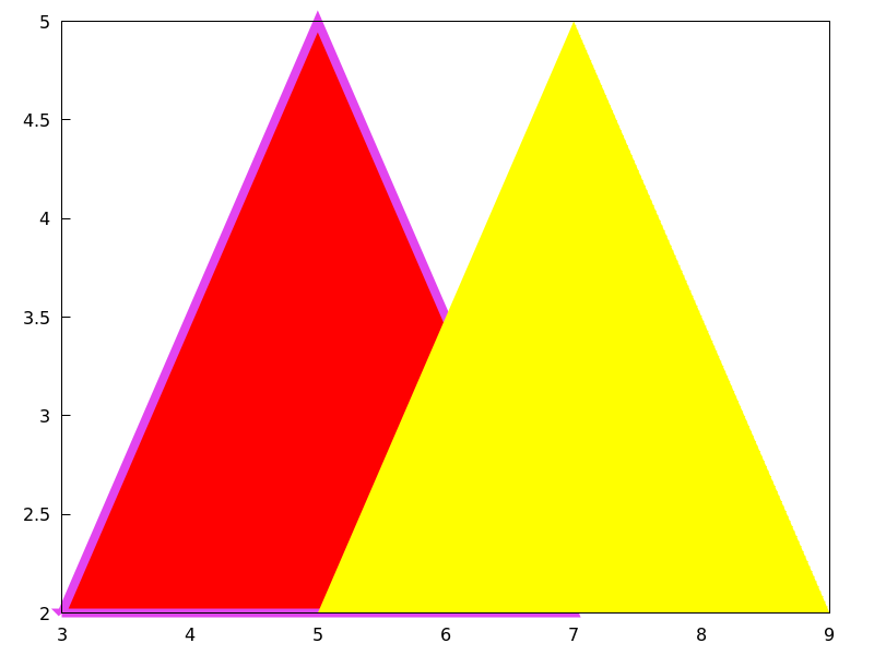

Categories: Package draw ·

Graphic object: quadrilateral (point_1, point_2, point_3, point_4) ¶

Draws a quadrilateral.

2D

quadrilateral([x1, y1], [x2, y2], [x3, y3], [x4, y4]) draws a quadrilateral with vertices [x1, y1], [x2, y2], [x3, y3], and [x4, y4].

This object is affected by the following graphic options:
transparent, fill_color, border, line_width, key, xaxis_secondary, yaxis_secondary, line_type, transform and color.

Example:

(%i1) draw2d(
        quadrilateral([1,1],[2,2],[3,-1],[2,-2]))$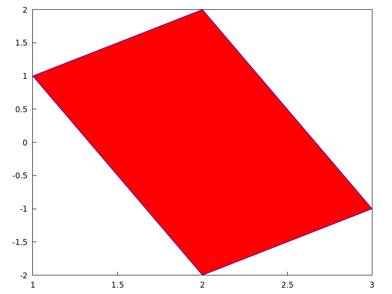

3D

quadrilateral([x1, y1, z1], [x2, y2, z2], [x3, y3, z3], [x4, y4, z4]) draws a quadrilateral with vertices [x1, y1, z1], [x2, y2, z2], [x3, y3, z3], and [x4, y4, z4].

This object is affected by the following graphic options: line_type, line_width, color, key, enhanced3d and transform.

Categories: Package draw ·

Graphic object: rectangle ([x1,y1], [x2,y2]) ¶

Draws rectangles in 2D.

2D

rectangle ([x1,y1], [x2,y2]) draws a rectangle with opposite vertices [x1,y1] and [x2,y2].

This object is affected by the following graphic options: transparent, fill_color, border, line_width, key, line_type and color.

Example:

(%i1) draw2d(fill_color  = red,
             line_width  = 6,
             line_type   = dots,
             transparent = false,
             fill_color  = blue,
             rectangle([-2,-2],[8,-1]), /* opposite vertices */
             transparent = true,
             line_type   = solid,
             line_width  = 1,
             rectangle([9,4],[2,-1.5]),
             xrange      = [-3,10],
             yrange      = [-3,4.5] )$

Categories: Package draw ·

Graphic object: region (expr,var1,minval1,maxval1,var2,minval2,maxval2) ¶

Plots a region on the plane defined by inequalities.

2D expr is an expression formed by inequalities and boolean operators and, or, and not. The region is bounded by the rectangle defined by [minval1, maxval1] and [minval2, maxval2].

This object is affected by the following graphic options: fill_color, fill_density, key, x_voxel and y_voxel.

Example:

(%i1) draw2d(
        x_voxel = 30,
        y_voxel = 30,
        region(x^2+y^2<1 and x^2+y^2 > 1/2,
               x, -1.5, 1.5, y, -1.5, 1.5));

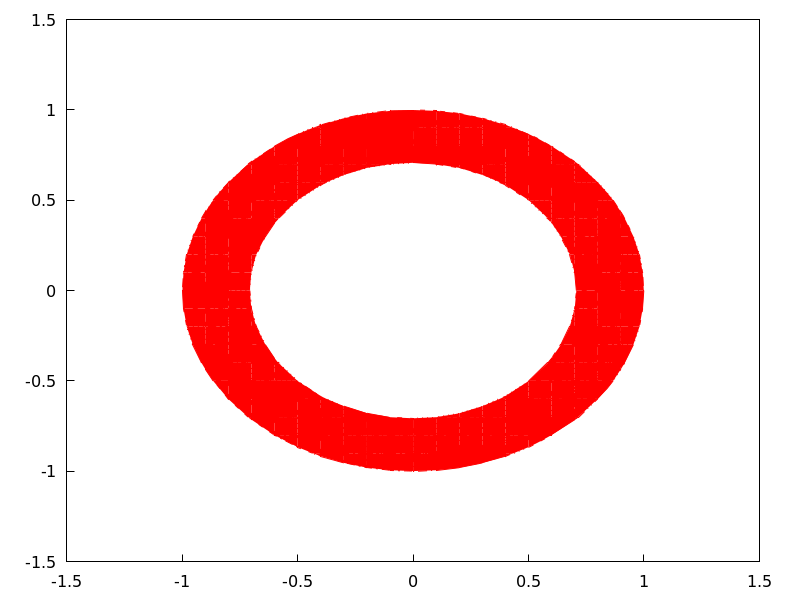
Graphic object: spherical (radius, azi, minazi, maxazi, zen, minzen, maxzen) ¶

Draws 3D functions defined in spherical coordinates.

3D

spherical(radius, azi, minazi, maxazi, zen, minzen, maxzen) plots the function radius(azi, zen) defined in spherical coordinates, with azimuth azi taking values from minazi to maxazi and zenith zen taking values from minzen to maxzen.

This object is affected by the following graphic options: xu_grid, yv_grid, line_type, key, wired_surface, enhanced3d and color.

Example:

(%i1) draw3d(spherical(1,a,0,2*%pi,z,0,%pi))$

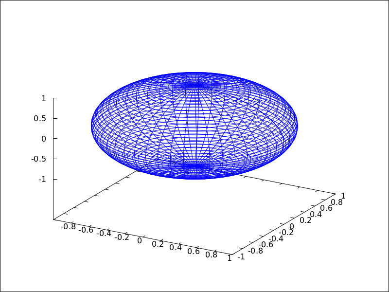Categories: Package draw ·

Graphic object: triangle (point_1, point_2, point_3) ¶

Draws a triangle.

2D

triangle ([x1,y1], [x2,y2], [x3,y3]) draws a triangle with vertices [x1,y1], [x2,y2], and [x3,y3].

This object is affected by the following graphic options:
transparent, fill_color, border, line_width, key, xaxis_secondary, yaxis_secondary, line_type, transform and color.

Example:

(%i1) draw2d(
        triangle([1,1],[2,2],[3,-1]))$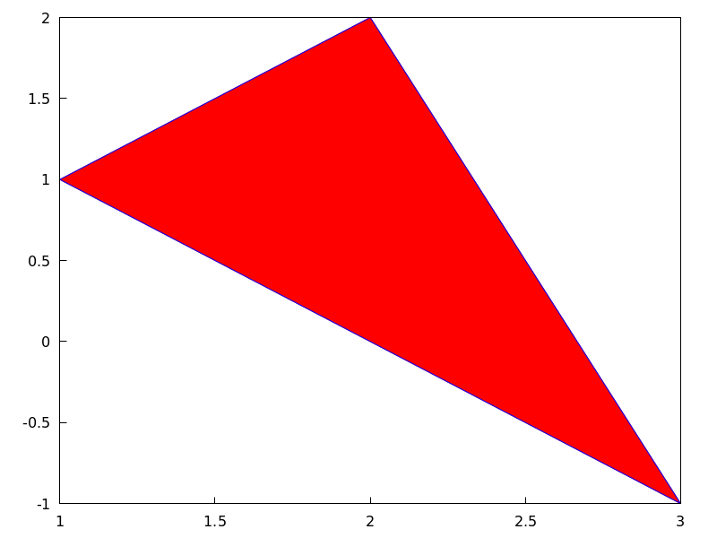

3D

triangle ([x1,y1,z1], [x2,y2,z2], [x3,y3,z3]) draws a triangle with vertices [x1,y1,z1], [x2,y2,z2], and [x3,y3,z3].

This object is affected by the following graphic options: line_type, line_width, color, key, enhanced3d and transform.

Categories: Package draw ·

Graphic object: tube (xfun,yfun,zfun,rfun,p,pmin,pmax) ¶

Draws a tube in 3D with varying diameter.

3D

[xfun,yfun,zfun] is the parametric curve with parameter p taking values from pmin to pmax. Circles of radius rfun are placed with their centers on the parametric curve and perpendicular to it.

This object is affected by the following graphic options: xu_grid, yv_grid, line_type, line_width, key, wired_surface, enhanced3d, color and capping.

Example:

(%i1) draw3d(
        enhanced3d = true,
        xu_grid = 50,
        tube(cos(a), a, 0, cos(a/10)^2,
             a, 0, 4*%pi) )$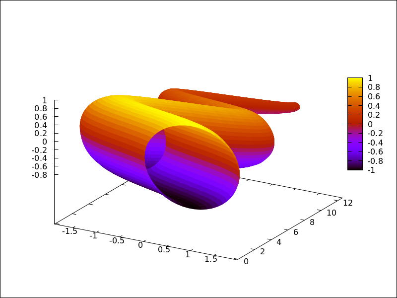

Categories: Package draw ·

Graphic object: vector
    vector ([x,y], [dx,dy])
    vector ([x,y,z], [dx,dy,dz]) ¶

Draws vectors in 2D and 3D.

This object is affected by the following graphic options: head_both, head_length, head_angle, head_type, line_width, line_type, key and color.

2D

vector([x,y], [dx,dy]) plots vector [dx,dy] with origin in [x,y].

Example:

(%i1) draw2d(xrange      = [0,12],
             yrange      = [0,10],
             head_length = 1,
             vector([0,1],[5,5]), /* default type */
             head_type = 'empty,
             vector([3,1],[5,5]),
             head_both = true,
             head_type = 'nofilled,
             line_type = dots,
             vector([6,1],[5,5]))$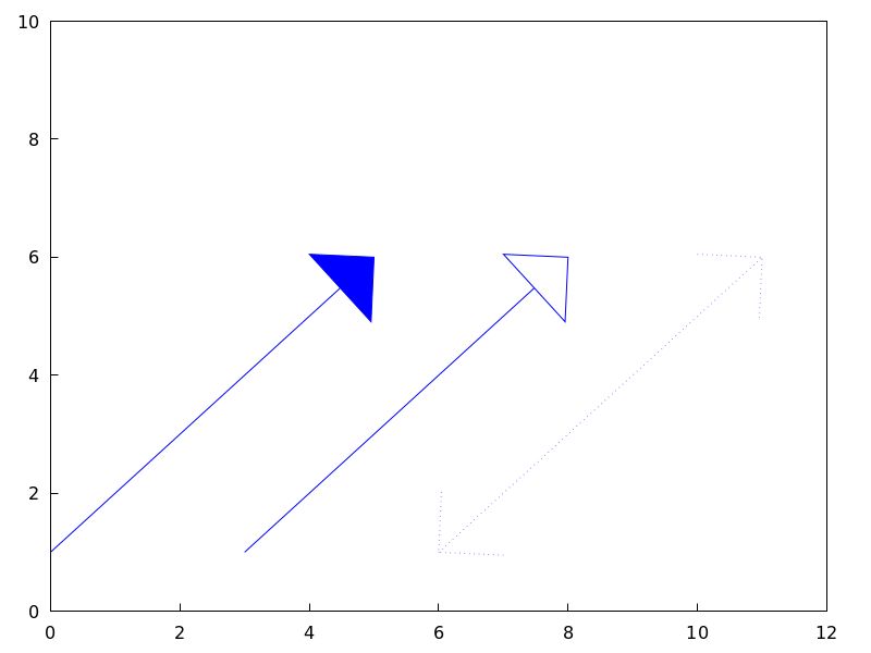

3D

vector([x,y,z], [dx,dy,dz]) plots vector [dx,dy,dz] with origin in [x,y,z].

Example:

(%i1) draw3d(color = cyan,
             vector([0,0,0],[1,1,1]/sqrt(3)),
             vector([0,0,0],[1,-1,0]/sqrt(2)),
             vector([0,0,0],[1,1,-2]/sqrt(6)) )$

Categories: Package draw ·

Variable: draw_renderer ¶

Default value: gnuplot_pipes

When draw_renderer is set to 'vtk, the VTK interface is used for draw.

Categories: Package draw ·