Next: Introduction to Maxima, Previous: (dir), Up: (dir) [Contents][Index]
Maxima is a computer algebra system, implemented in Lisp.
Maxima is derived from the Macsyma system, developed at MIT in the years 1968 through 1982 as part of Project MAC. MIT turned over a copy of the Macsyma source code to the Department of Energy in 1982; that version is now known as DOE Macsyma. A copy of DOE Macsyma was maintained by Professor William F. Schelter of the University of Texas from 1982 until his death in 2001. In 1998, Schelter obtained permission from the Department of Energy to release the DOE Macsyma source code under the GNU Public License, and in 2000 he initiated the Maxima project at SourceForge to maintain and develop DOE Macsyma, now called Maxima.
Table of Contents
- 1 Introduction to Maxima
- 2 Command-line options
- 3 Runtime Environment
- 4 Bug Detection and Reporting
- 5 Help
- 6 Command Line
- 7 Data Types and Structures
- 8 Expressions
- 9 Operators
- 10 Evaluation
- 11 Simplification
- 12 Elementary Functions
- 13 Maxima’s Database
- 14 Plotting
- 15 File Input and Output
- 16 Polynomials
- 17 Special Functions
- 17.1 Introduction to Special Functions
- 17.2 Bessel Functions
- 17.3 Airy Functions
- 17.4 Gamma and Factorial Functions
- 17.5 Exponential Integrals
- 17.6 Error Function
- 17.7 Struve Functions
- 17.8 Hypergeometric Functions
- 17.9 Parabolic Cylinder Functions
- 17.10 Functions and Variables for Special Functions
- 18 Elliptic Functions
- 19 Limits
- 20 Differentiation
- 21 Integration
- 22 Equations
- 23 Differential Equations
- 24 Numerical
- 24.1 Introduction to fast Fourier transform
- 24.2 Functions and Variables for fft
- 24.3 Functions and Variables for FFTPACK5
- 24.4 Functions for numerical solution of equations
- 24.5 Introduction to numerical solution of differential equations
- 24.6 Functions for numerical solution of differential equations
- 25 Matrices and Linear Algebra
- 26 Sums, Products, and Series
- 27 Number Theory
- 28 Groups
- 29 Miscellaneous Options
- 30 Rules and Patterns
- 31 Sets
- 32 Function Definition
- 33 Program Flow
- 34 Debugging
- 35 Error and warning messages
- 35.1 Error Messages
- 35.1.1 apply: no such "list" element
- 35.1.2 argument must be a non-atomic expression
- 35.1.3 assignment: cannot assign to
<function name> - 35.1.4 expt: undefined: 0 to a negative exponent.
- 35.1.5 incorrect syntax: , is not a prefix operator
- 35.1.6 incorrect syntax: Illegal use of delimiter )
- 35.1.7 loadfile: failed to load
<filename> - 35.1.8 makelist: second argument must evaluate to a number
- 35.1.9 Only symbols can be bound
- 35.1.10 operators of arguments must all be the same
- 35.1.11 Out of memory
- 35.1.12 part: fell off the end
- 35.1.13 undefined variable (draw or plot)
- 35.1.14 VTK is not installed, which is required for Scene
- 35.2 Warning Messages
- 35.1 Error Messages
- 36 Package affine
- 37 Package alt-display
- 38 Package asympa
- 39 Package atensor
- 40 Package augmented_lagrangian
- 41 Package bernstein
- 42 Package bitwise
- 43 Package bode
- 44 Package cartan
- 45 Package celine
- 46 Package clebsch_gordan
- 47 Package cobyla
- 48 Package colnew
- 49 Package combinatorics
- 50 Package contrib_ode
- 51 Package ctensor
- 51.1 Introduction to ctensor
- 51.2 Functions and Variables for ctensor
- 51.2.1 Initialization and setup
- 51.2.2 The tensors of curved space
- 51.2.3 Taylor series expansion
- 51.2.4 Frame fields
- 51.2.5 Algebraic classification
- 51.2.6 Torsion and nonmetricity
- 51.2.7 Miscellaneous features
- 51.2.8 Utility functions
- 51.2.9 Variables used by
ctensor - 51.2.10 Reserved names
- 51.2.11 Changes
- 52 Package descriptive
- 53 Package diag
- 54 Package distrib
- 54.1 Introduction to distrib
- 54.2 Functions and Variables for continuous distributions
- 54.2.1 Normal Random Variable
- 54.2.2 Student’s t Random Variable
- 54.2.3 Noncentral Student’s t Random Variable
- 54.2.4 Chi-squared Random Variable
- 54.2.5 Noncentral Chi-squared Random Variable
- 54.2.6 F Random Variable
- 54.2.7 Exponential Random Variable
- 54.2.8 Lognormal Random Variable
- 54.2.9 Gamma Random Variable
- 54.2.10 Beta Random Variable
- 54.2.11 Continuous Uniform Random Variable
- 54.2.12 Logistic Random Variable
- 54.2.13 Pareto Random Variable
- 54.2.14 Weibull Random Variable
- 54.2.15 Rayleigh Random Variable
- 54.2.16 Laplace Random Variable
- 54.2.17 Cauchy Random Variable
- 54.2.18 Gumbel Random Variable
- 54.3 Functions and Variables for discrete distributions
- 55 Package draw
- 56 Package drawdf
- 57 Package dynamics
- 58 Package engineering-format
- 59 Package ezunits
- 60 Package f90
- 61 Package finance
- 62 Package format
- 63 Package fractals
- 64 Package gentran
- 65 Package ggf
- 66 Package graphs
- 67 Package grobner
- 68 Package hompack
- 69 Package impdiff
- 70 Package interpol
- 71 Package itensor
- 72 Package lapack
- 73 Package lbfgs
- 74 Package levin
- 75 Package lindstedt
- 76 Package linearalgebra
- 77 Package lsquares
- 78 Package minpack
- 79 Package makeOrders
- 80 Package mnewton
- 81 Package numericalio
- 82 Package odepack
- 83 Package operatingsystem
- 84 Package opsubst
- 85 Package orthopoly
- 86 Package pslq
- 87 Package pytranslate
- 88 Package quantum_computing
- 89 Package ratpow
- 90 Package romberg
- 91 Package simplex
- 92 Package simplification
- 93 Package solve_rec
- 94 Package stats
- 95 Package stirling
- 96 Package stringproc
- 97 Package sym
- 98 Package to_poly_solve
- 99 Package trigtools
- 100 Package unit
- 101 Package wrstcse
- 102 Package zeilberger
- Appendix A Function and Variable Index
- Appendix B Documentation Categories
Short Table of Contents
- 1 Introduction to Maxima
- 2 Command-line options
- 3 Runtime Environment
- 4 Bug Detection and Reporting
- 5 Help
- 6 Command Line
- 7 Data Types and Structures
- 8 Expressions
- 9 Operators
- 10 Evaluation
- 11 Simplification
- 12 Elementary Functions
- 13 Maxima’s Database
- 14 Plotting
- 15 File Input and Output
- 16 Polynomials
- 17 Special Functions
- 18 Elliptic Functions
- 19 Limits
- 20 Differentiation
- 21 Integration
- 22 Equations
- 23 Differential Equations
- 24 Numerical
- 25 Matrices and Linear Algebra
- 26 Sums, Products, and Series
- 27 Number Theory
- 28 Groups
- 29 Miscellaneous Options
- 30 Rules and Patterns
- 31 Sets
- 32 Function Definition
- 33 Program Flow
- 34 Debugging
- 35 Error and warning messages
- 36 Package affine
- 37 Package alt-display
- 38 Package asympa
- 39 Package atensor
- 40 Package augmented_lagrangian
- 41 Package bernstein
- 42 Package bitwise
- 43 Package bode
- 44 Package cartan
- 45 Package celine
- 46 Package clebsch_gordan
- 47 Package cobyla
- 48 Package colnew
- 49 Package combinatorics
- 50 Package contrib_ode
- 51 Package ctensor
- 52 Package descriptive
- 53 Package diag
- 54 Package distrib
- 55 Package draw
- 56 Package drawdf
- 57 Package dynamics
- 58 Package engineering-format
- 59 Package ezunits
- 60 Package f90
- 61 Package finance
- 62 Package format
- 63 Package fractals
- 64 Package gentran
- 65 Package ggf
- 66 Package graphs
- 67 Package grobner
- 68 Package hompack
- 69 Package impdiff
- 70 Package interpol
- 71 Package itensor
- 72 Package lapack
- 73 Package lbfgs
- 74 Package levin
- 75 Package lindstedt
- 76 Package linearalgebra
- 77 Package lsquares
- 78 Package minpack
- 79 Package makeOrders
- 80 Package mnewton
- 81 Package numericalio
- 82 Package odepack
- 83 Package operatingsystem
- 84 Package opsubst
- 85 Package orthopoly
- 86 Package pslq
- 87 Package pytranslate
- 88 Package quantum_computing
- 89 Package ratpow
- 90 Package romberg
- 91 Package simplex
- 92 Package simplification
- 93 Package solve_rec
- 94 Package stats
- 95 Package stirling
- 96 Package stringproc
- 97 Package sym
- 98 Package to_poly_solve
- 99 Package trigtools
- 100 Package unit
- 101 Package wrstcse
- 102 Package zeilberger
- Appendix A Function and Variable Index
- Appendix B Documentation Categories
Next: Command-line options [Contents][Index]
1 Introduction to Maxima
Start Maxima with the command "maxima". Maxima will display version
information and a prompt. End each Maxima command with a semicolon.
End the session with the command "quit();". Here’s a sample session:
$ maxima
Maxima 5.45.1 https://maxima.sourceforge.io
using Lisp SBCL 2.0.1.debian
Distributed under the GNU Public License. See the file COPYING.
Dedicated to the memory of William Schelter.
The function bug_report() provides bug reporting information.
(%i1) factor(10!);
8 4 2
(%o1) 2 3 5 7
(%i2) expand ((x + y)^6);
6 5 2 4 3 3 4 2 5 6
(%o2) y + 6 x y + 15 x y + 20 x y + 15 x y + 6 x y + x
(%i3) factor (x^6 - 1);
2 2
(%o3) (x - 1) (x + 1) (x - x + 1) (x + x + 1)
(%i4) quit();
$
Maxima can search the info pages. Use the describe command to show
information about the command or all the commands and variables containing
a string.
The question mark ? (exact search) and double question mark ??
(inexact search) are abbreviations for describe:
(%i1) ?? integ
0: Functions and Variables for Elliptic Integrals
1: Functions and Variables for Integration
2: Introduction to Elliptic Functions and Integrals
3: Introduction to Integration
4: askinteger (Functions and Variables for Simplification)
5: integerp (Functions and Variables for Miscellaneous Options)
6: integer_partitions (Functions and Variables for Sets)
7: integrate (Functions and Variables for Integration)
8: integrate_use_rootsof (Functions and Variables for Integration)
9: integration_constant_counter (Functions and Variables for
Integration)
10: nonnegintegerp (Functions and Variables for linearalgebra)
Enter space-separated numbers, `all' or `none': 5 4
-- Function: integerp (<expr>)
Returns `true' if <expr> is a literal numeric integer, otherwise
`false'.
`integerp' returns false if its argument is a symbol, even if the
argument is declared integer.
Examples:
(%i1) integerp (0);
(%o1) true
(%i2) integerp (1);
(%o2) true
(%i3) integerp (-17);
(%o3) true
(%i4) integerp (0.0);
(%o4) false
(%i5) integerp (1.0);
(%o5) false
(%i6) integerp (%pi);
(%o6) false
(%i7) integerp (n);
(%o7) false
(%i8) declare (n, integer);
(%o8) done
(%i9) integerp (n);
(%o9) false
-- Function: askinteger (<expr>, integer)
-- Function: askinteger (<expr>)
-- Function: askinteger (<expr>, even)
-- Function: askinteger (<expr>, odd)
`askinteger (<expr>, integer)' attempts to determine from the
`assume' database whether <expr> is an integer. `askinteger'
prompts the user if it cannot tell otherwise, and attempt to
install the information in the database if possible. `askinteger
(<expr>)' is equivalent to `askinteger (<expr>, integer)'.
`askinteger (<expr>, even)' and `askinteger (<expr>, odd)'
likewise attempt to determine if <expr> is an even integer or odd
integer, respectively.
(%o1) true
To use a result in later calculations, you can assign it to a variable or
refer to it by its automatically supplied label. In addition, %
refers to the most recent calculated result:
(%i1) u: expand ((x + y)^6);
6 5 2 4 3 3 4 2 5 6
(%o1) y + 6 x y + 15 x y + 20 x y + 15 x y + 6 x y + x
(%i2) diff (u, x);
5 4 2 3 3 2 4 5
(%o2) 6 y + 30 x y + 60 x y + 60 x y + 30 x y + 6 x
(%i3) factor (%o2);
5
(%o3) 6 (y + x)
Maxima knows about complex numbers and numerical constants:
(%i1) cos(%pi); (%o1) - 1
(%i2) exp(%i*%pi); (%o2) - 1
Maxima can do differential and integral calculus:
(%i1) u: expand ((x + y)^6);
6 5 2 4 3 3 4 2 5 6
(%o1) y + 6 x y + 15 x y + 20 x y + 15 x y + 6 x y + x
(%i2) diff (%, x);
5 4 2 3 3 2 4 5
(%o2) 6 y + 30 x y + 60 x y + 60 x y + 30 x y + 6 x
(%i3) integrate (1/(1 + x^3), x);
2 x - 1
2 atan(-------)
log(x - x + 1) sqrt(3) log(x + 1)
(%o3) - --------------- + ------------- + ----------
6 sqrt(3) 3
Maxima can solve linear systems and cubic equations:
(%i1) linsolve ([3*x + 4*y = 7, 2*x + a*y = 13], [x, y]);
7 a - 52 25
(%o1) [x = --------, y = -------]
3 a - 8 3 a - 8
(%i2) solve (x^3 - 3*x^2 + 5*x = 15, x); (%o2) [x = - sqrt(5) %i, x = sqrt(5) %i, x = 3]
Maxima can solve nonlinear sets of equations. Note that if you don’t want a result printed, you can finish your command with $ instead of ;.
(%i1) eq_1: x^2 + 3*x*y + y^2 = 0$ (%i2) eq_2: 3*x + y = 1$
(%i3) solve ([eq_1, eq_2]);
3 sqrt(5) + 7 sqrt(5) + 3
(%o3) [[y = - -------------, x = -----------],
2 2
3 sqrt(5) - 7 sqrt(5) - 3
[y = -------------, x = - -----------]]
2 2
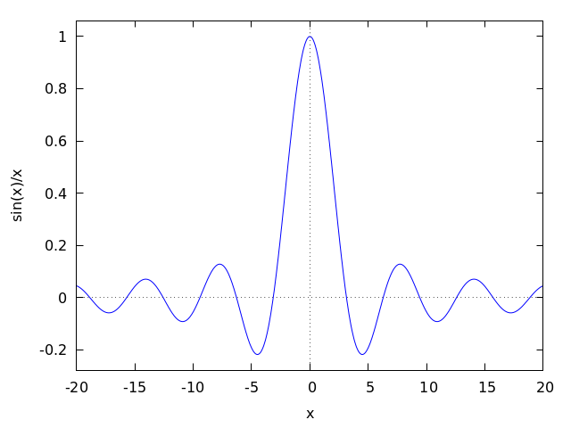
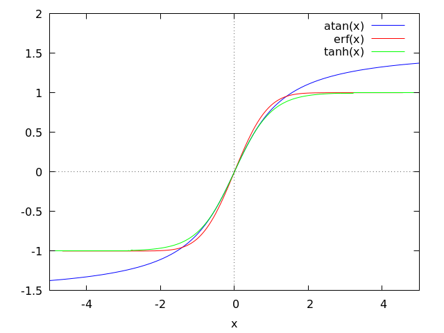
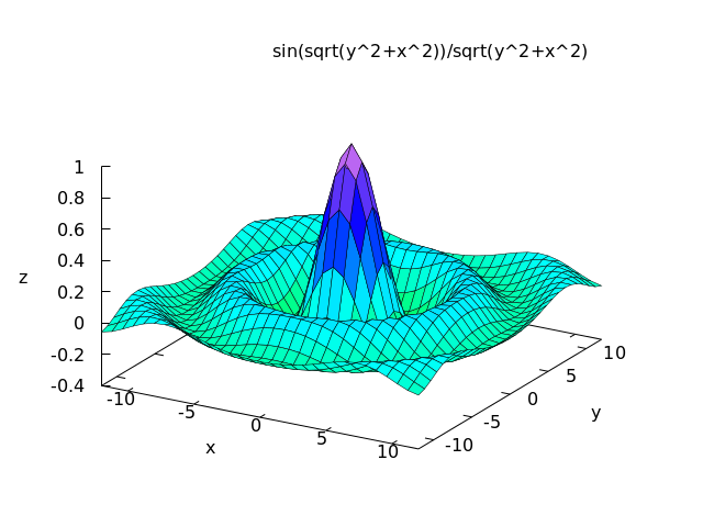
Maxima can generate plots of one or more functions:
(%i1) plot2d (sin(x)/x, [x, -20, 20])$
(%i2) plot2d ([atan(x), erf(x), tanh(x)], [x, -5, 5], [y, -1.5, 2])$
(%i3) plot3d (sin(sqrt(x^2 + y^2))/sqrt(x^2 + y^2),
[x, -12, 12], [y, -12, 12])$
Next: Runtime Environment, Previous: Introduction to Maxima [Contents][Index]
2 Command-line options
The following command line options are available for Maxima:
-b <file>, --batch=<file>Process maxima file <file> in batch mode.
--batch-lisp=<file>Process lisp file <file> in batch mode.
--batch-string=<string>Process maxima command(s) <string> in batch mode.
-d, --directoriesDisplay maxima internal directory information.
--disable-readlineDisable readline support.
-g, --enable-lisp-debuggerEnable underlying lisp debugger.
-h, --helpDisplay this usage message.
--userdir=<directory>Use <directory> for user directory (default is %USERPROFILE%/maxima for Windows, and $HOME/.maxima for other operating systems).
--init=<file>Set the base name of the Maxima & Lisp initialization files (default is "maxima-init".) The last extension and any directory parts are removed to form the base name. The resulting files, <base>.mac and <base>.lisp are only searched for in userdir (see –userdir option). This may be specified for than once, but only the last is used.
-l <lisp>, --lisp=<lisp>Use lisp implementation <lisp>.
--list-availList the installed version/lisp combinations.
-p <file>, --preload=<file>, --preload-lisp=<file>, --init-mac=<file>, --init-lisp=<file>Preload <file>, which may be any file time accepted by Maxima’s LOAD function. The <file> is loaded before any other system initialization is done. This will be searched for in the locations given by file_search_maxima and file_search_lisp. This can be specified multiple times to load multiple files. The equivalent options –preload-lisp, –init-mac, and –init-lisp are deprecated.
-q, --quietSuppress Maxima start-up message.
-Q, --quit-on-errorQuit, and return an exit code 1, when Maxima encounters an error.
-r <string>, --run-string=<string>Process maxima command(s) <string> in interactive mode.
-s <port>, --server=<port>Connect Maxima to server on <port>.
--suppress-input-echoDo not print input expressions when processing noninteractively.
-u <version>, --use-version=<version>Use maxima version <version>.
-v, --verboseDisplay lisp invocation in maxima wrapper script.
--versionDisplay the default installed version.
--very-quietSuppress expression labels, Maxima start-up message and verification of html index.
--very-very-quietIn addition to –very-quiet, suppress most printed output by setting TTYOFF to T.
-X <Lisp options>, --lisp-options=<Lisp options>Options to be given to the underlying Lisp
--no-init, --norcDo not load the init file(s) on startup
--verify-html-indexVerify on startup that the set of html topics is consistent with text topics.
Next: Bug Detection and Reporting, Previous: Command-line options [Contents][Index]
3 Runtime Environment
Next: Interrupts, Previous: Runtime Environment, Up: Runtime Environment [Contents][Index]
3.1 Introduction for Runtime Environment
maxima-init.mac and maxima-init.lisp are loaded automatically when Maxima
starts. maxima-init.mac contains Maxima code and is loaded using batchload,
maxima-init.lisp contains Lisp code and is loaded using load.
You can use maxima-init.mac (and maxima-init.lisp) to customize your Maxima
environment. These files typically placed in the directory named by
maxima_userdir, although it can be in any directory searched by the function
file_search.
Here is an example maxima-init.mac file:
setup_autoload ("specfun.mac", ultraspherical, assoc_legendre_p);
showtime:all;
In this example, setup_autoload tells Maxima to load the
specified file
(specfun.mac) if any of the functions (ultraspherical,
assoc_legendre_p) are called but not yet defined.
Thus you needn’t remember to load the file before calling the functions.
The statement showtime: all tells Maxima to set the showtime
variable. The maxima-init.mac file can contain any other assignments or
other Maxima statements.
maxima-init.mac and maxima-init.lisp are loaded automatically when Maxima
starts. maxima-init.mac contains Maxima code and is loaded using batchload,
maxima-init.lisp contains Lisp code and is loaded using load.
maximarc is sourced by the maxima script at startup. It should be located in $MAXIMA_USERDIR.
If Maxima was compiled with several Lisp compilers, maximarc can be used, e.g., to change the
user’s default lisp implementation. E.g. to select CMUCL create a maximarc file containing the line:
MAXIMA_LISP=cmucl
You can also use the command option -l <lisp> or --lisp=<lisp> to select the Lisp when starting Maxima.
If you run Maxima using the graphical interface Xmaxima, the default
configuration of that interface will be saved in the file
xmaxima_default and the history of the last 200 commands will be
saved in the file xmaxima_history in a sub-directory maxima (or
Maxima in Windows) of the user’s local configuration directory.
In Linux systems, the user’s local configuration directory is usually
/home/<username>/.config and in Windows systems it is usually
<Drive_letter>:/Users/<username>/AppData/Local. Notice that in
both systems those directories are hidden, and their default value can
be changed with an environment variable (XDG_CONFIG_HOME in Linux
or LOCALAPPDATA in Windows). If the local configuration directory
is not found, those two files will be saved in the users home directory
and with the names .xmaximarc and .xmaxima_history, as in
older versions of Xmaxima.
Next: Functions and Variables for Runtime Environment, Previous: Introduction for Runtime Environment, Up: Runtime Environment [Contents][Index]
3.2 Interrupts
The user can stop a time-consuming computation with the ^C (control-C) character. The default action is to stop the computation and print another user prompt. In this case, it is not possible to restart a stopped computation.
If the Lisp variable *debugger-hook* is set to nil, by executing
:lisp (setq *debugger-hook* nil)
then upon receiving ^C, Maxima will enter the Lisp debugger,
and the user may use the debugger to inspect the Lisp environment.
The stopped computation can be restarted by entering
continue in the Lisp debugger.
The means of returning to Maxima from the Lisp debugger
(other than running the computation to completion)
is different for each version of Lisp.
On Unix systems, the character ^Z (control-Z) causes Maxima
to stop altogether, and control is returned to the shell prompt.
The fg command causes Maxima
to resume from the point at which it was stopped.
Previous: Interrupts, Up: Runtime Environment [Contents][Index]
3.3 Functions and Variables for Runtime Environment
- System variable: maxima_tempdir 
-
maxima_tempdirnames the directory in which Maxima creates some temporary files. In particular, temporary files for plotting are created inmaxima_tempdir.The initial value of
maxima_tempdiris the user’s home directory, if Maxima can locate it; otherwise Maxima makes a guess about a suitable directory.maxima_tempdirmay be assigned a string which names a directory.Categories: Global variables ·
- System variable: maxima_userdir 
-
maxima_userdirnames a directory which Maxima searches to find Maxima and Lisp files. (Maxima searches some other directories as well;file_search_maximaandfile_search_lispare the complete lists.)The initial value of
maxima_userdiris a subdirectory of the user’s home directory, if Maxima can locate it; otherwise Maxima makes a guess about a suitable directory.maxima_userdirmay be assigned a string which names a directory. However, assigning tomaxima_userdirdoes not automatically changefile_search_maximaandfile_search_lisp; those variables must be changed separately.Categories: Global variables ·
- Function: room
room ()
room (true)
room (false) ¶ -
Prints out a description of the state of storage and stack management in Maxima.
roomcalls the Lisp function of the same name.-
room ()prints out a moderate description. -
room (true)prints out a verbose description. -
room (false)prints out a terse description.
Categories: Debugging · -
- Function: sstatus (keyword, item) 
-
When keyword is the symbol
feature, item is put on the list of system features. Aftersstatus (keyword, item)is executed,status (feature, item)returnstrue. If keyword is the symbolnofeature, item is deleted from the list of system features. This can be useful for package writers, to keep track of what features they have loaded in.See also
status.Categories: Programming ·
- Function: status
status (feature)
status (feature, item) ¶ -
Returns information about the presence or absence of certain system-dependent features.
-
status (feature)returns a list of system features. These include Lisp version, operating system type, etc. The list may vary from one Lisp type to another. -
status (feature, item)returnstrueif item is on the list of items returned bystatus (feature)andfalseotherwise.statusquotes the argument item. The quote-quote operator''defeats quotation. A feature whose name contains a special character, such as a hyphen, must be given as a string argument. For example,status (feature, "ansi-cl").
See also
sstatus.The variable
featurescontains a list of features which apply to mathematical expressions. Seefeaturesandfeaturepfor more information.Categories: Programming · -
- Function: system
system (command, arg_1, ..., arg_n)
system (command) ¶ -
Executes command as a separate process. The command is passed to the default shell for execution.
systemis implemented by a command execution function in the Lisp implementation which compiled Maxima, and therefore the behavior ofsystemvaries with the operating system and Lisp implementation.systemis known to work on Windows and Linux systems, and might also work on other systems.All combinations of Lisp implementation and operating system allow command arguments as arg_1, ..., arg_n, and some allow command arguments as part of command. SBCL on Windows and Clozure CL on Windows are known to require command arguments to be specified as arg_1, ..., arg_n.
systemdoes not attempt to quote or escape spaces or other characters in command or in arg_1, ..., arg_n; all arguments are supplied verbatim to the command execution function of the Lisp implementation.Standard output from command is displayed on the Maxima console by default, and may be captured by
with_stdout.For most Lisp implementations, the call to
systemreturns after command has completed. Job control operations, such as executing a command asynchronously with respect to Maxima, are not known to have the expected effect.Examples:
systemexecutes command as a separate process. The output of the commanddirvaries from one system to another.(%i1) system ("dir", maxima_tempdir); config-err-UsLLQM gnome-software-0TNK22 MozillaUpdateLock-6939C585ADF59520 snap-private-tmp systemd-private-169e359ab2d94b208622fa96dd88c05e-colord.service-ZP9Xn7 (%o1) 0All combinations of Lisp implementation and operating system allow command arguments as arg_1, ..., arg_n.
(%i1) system ("echo", "Hello", "world", "glad", "to", "meet", "you"); Hello world glad to meet you (%o1) 0Standard output from command is displayed on the Maxima console by default, and may be captured by
with_stdout.(%i1) my_output: sconcat (maxima_tempdir, "/tmp.out"); (%o1) /tmp/tmp.out (%i2) with_stdout (my_output, system ("dir")); (%o2) 0 (%i3) S: openr (my_output); (%o3) #<FILE-STREAM {7B500975}> (%i4) readline (S); (%o4) aclocal.m4 (%i5) readline (S); (%o5) admin (%i6) readline (S); (%o6) archiveFor most Lisp implementations, the call to
systemreturns after command has completed.xfontselis a utility to inspect fonts for the X Windows system;systemreturns after the user clicks the "quit" button.(%i1) system ("xfontsel"); (%o1) 0
- Function: time (%o1, %o2, %o3, …) 
-
Returns a list of the times, in seconds, taken to compute the output lines
%o1,%o2,%o3, … The time returned is Maxima’s estimate of the internal computation time, not the elapsed time.timecan only be applied to output line variables; for any other variables,timereturnsunknown.Set
showtime: trueto make Maxima print out the computation time and elapsed time with each output line.Categories: Debugging ·
- Function: timedate
timedate (T, tz_offset)
timedate (T)
timedate () ¶ -
timedate(T, tz_offset)returns a string representing the time T in the time zone tz_offset. The string format isYYYY-MM-DD HH:MM:SS.NNN[+|-]ZZ:ZZ(using as many digits as necessary to represent the fractional part) if T has a nonzero fractional part, orYYYY-MM-DD HH:MM:SS[+|-]ZZ:ZZif its fractional part is zero.T measures time, in seconds, since midnight, January 1, 1900, in the GMT time zone.
tz_offset measures the offset of the time zone, in hours, east (positive) or west (negative) of GMT. tz_offset must be an integer, rational, or float between -24 and 24, inclusive. If tz_offset is not a multiple of 1/60, it is rounded to the nearest multiple of 1/60.
timedate(T)is equivalent totimedate(T, tz_offset)with tz_offset equal to the offset of the local time zone.timedate()is equivalent totimedate(absolute_real_time()). That is, it returns the current time in the local time zone.Example:
timedatewith no argument returns a string representing the current time and date.(%i1) d : timedate (); (%o1) 2010-06-08 04:08:09+01:00 (%i2) print ("timedate reports current time", d) $ timedate reports current time 2010-06-08 04:08:09+01:00timedatewith an argument returns a string representing the argument.(%i1) timedate (0); (%o1) 1900-01-01 01:00:00+01:00 (%i2) timedate (absolute_real_time () - 7*24*3600); (%o2) 2010-06-01 04:19:51+01:00
timedatewith optional timezone offset.(%i1) timedate (1000000000, -9.5); (%o1) 1931-09-09 16:16:40-09:30
Categories: Time and date functions ·
- Function: parse_timedate
parse_timedate (S) ¶ -
Parses a string S representing a date or date and time of day and returns the number of seconds since midnight, January 1, 1900 GMT. If there is a nonzero fractional part, the value returned is a rational number, otherwise, it is an integer.
parse_timedatereturnsfalseif it cannot parse S according to any of the allowed formats.The string S must have one of the following formats, optionally followed by a timezone designation:
-
YYYY-MM-DD[ T]hh:mm:ss[,.]nnn -
YYYY-MM-DD[ T]hh:mm:ss -
YYYY-MM-DD
where the fields are year, month, day, hours, minutes, seconds, and fraction of a second, and square brackets indicate acceptable alternatives. The fraction may contain one or more digits.
Except for the fraction of a second, each field must have exactly the number of digits indicated: four digits for the year, and two for the month, day of the month, hours, minutes, and seconds.
A timezone designation must have one of the following forms:
-
[+-]hh:mm -
[+-]hhmm -
[+-]hh -
Z
where
hhandmmindicate hours and minutes east (+) or west (-) of GMT. The timezone may be from +24 hours (inclusive) to -24 hours (inclusive).A literal character
Zis equivalent to+00:00and its variants, indicating GMT.If no timezone is indicated, the time is assumed to be in the local time zone.
Any leading or trailing whitespace (space, tab, newline, and carriage return) is ignored, but any other leading or trailing characters cause
parse_timedateto fail and returnfalse.See also
timedateandabsolute_real_time.Examples:
Midnight, January 1, 1900, in the local time zone, in each acceptable format. The result is the number of seconds the local time zone is ahead (negative result) or behind (positive result) GMT. In this example, the local time zone is 8 hours behind GMT.
(%i1) parse_timedate ("1900-01-01 00:00:00,000"); (%o1) 28800 (%i2) parse_timedate ("1900-01-01 00:00:00.000"); (%o2) 28800 (%i3) parse_timedate ("1900-01-01T00:00:00,000"); (%o3) 28800 (%i4) parse_timedate ("1900-01-01T00:00:00.000"); (%o4) 28800 (%i5) parse_timedate ("1900-01-01 00:00:00"); (%o5) 28800 (%i6) parse_timedate ("1900-01-01T00:00:00"); (%o6) 28800 (%i7) parse_timedate ("1900-01-01"); (%o7) 28800Midnight, January 1, 1900, GMT, in different indicated time zones.
(%i1) parse_timedate ("1900-01-01 19:00:00+19:00"); (%o1) 0 (%i2) parse_timedate ("1900-01-01 07:00:00+07:00"); (%o2) 0 (%i3) parse_timedate ("1900-01-01 01:00:00+01:00"); (%o3) 0 (%i4) parse_timedate ("1900-01-01Z"); (%o4) 0 (%i5) parse_timedate ("1899-12-31 21:00:00-03:00"); (%o5) 0 (%i6) parse_timedate ("1899-12-31 13:00:00-11:00"); (%o6) 0 (%i7) parse_timedate ("1899-12-31 08:00:00-16:00"); (%o7) 0Categories: Time and date functions · -
- Function: encode_time
encode_time (year, month, day, hours, minutes, seconds, tz_offset)
encode_time (year, month, day, hours, minutes, seconds) ¶ -
Given a time and date specified by year, month, day, hours, minutes, and seconds,
encode_timereturns the number of seconds (possibly including a fractional part) since midnight, January 1, 1900 GMT.year must be an integer greater than or equal to 1899. However, 1899 is allowed only if the resulting encoded time is greater than or equal to 0.
month must be an integer from 1 to 12, inclusive.
day must be an integer from 1 to n, inclusive, where n is the number of days in the month specified by month.
hours must be an integer from 0 to 23, inclusive.
minutes must be an integer from 0 to 59, inclusive.
seconds must be an integer, rational, or float greater than or equal to 0 and less than 60. When seconds is not an integer,
encode_timereturns a rational, such that the fractional part of the return value is equal to the fractional part of seconds. Otherwise, seconds is an integer, and the return value is likewise an integer.tz_offset measures the offset of the time zone, in hours, east (positive) or west (negative) of GMT. tz_offset must be an integer, rational, or float between -24 and 24, inclusive. If tz_offset is not a multiple of 1/3600, it is rounded to the nearest multiple of 1/3600.
If tz_offset is not present, the offset of the local time zone is assumed.
See also
decode_time.Examples:
(%i1) encode_time (1900, 1, 1, 0, 0, 0, 0); (%o1) 0 (%i2) encode_time (1970, 1, 1, 0, 0, 0, 0); (%o2) 2208988800 (%i3) encode_time (1970, 1, 1, 8, 30, 0, 8.5); (%o3) 2208988800 (%i4) encode_time (1969, 12, 31, 16, 0, 0, -8); (%o4) 2208988800 (%i5) encode_time (1969, 12, 31, 16, 0, 1/1000, -8); 2208988800001 (%o5) ------------- 1000 (%i6) % - 2208988800; 1 (%o6) ---- 1000Categories: Time and date functions ·
- Function: decode_time
decode_time (T, tz_offset)
decode_time (T) ¶ -
Given the number of seconds (possibly including a fractional part) since midnight, January 1, 1900 GMT, returns the date and time as represented by a list comprising the year, month, day of the month, hours, minutes, seconds, and time zone offset.
tz_offset measures the offset of the time zone, in hours, east (positive) or west (negative) of GMT. tz_offset must be an integer, rational, or float between -24 and 24, inclusive. If tz_offset is not a multiple of 1/3600, it is rounded to the nearest multiple of 1/3600.
If tz_offset is not present, the offset of the local time zone is assumed.
See also
encode_time.Examples:
(%i1) decode_time (0, 0); (%o1) [1900, 1, 1, 0, 0, 0, 0] (%i2) decode_time (0); (%o2) [1899, 12, 31, 16, 0, 0, - 8] (%i3) decode_time (2208988800, 9.25); 37 (%o3) [1970, 1, 1, 9, 15, 0, --] 4 (%i4) decode_time (2208988800); (%o4) [1969, 12, 31, 16, 0, 0, - 8] (%i5) decode_time (2208988800 + 1729/1000, -6); 1729 (%o5) [1969, 12, 31, 18, 0, ----, - 6] 1000 (%i6) decode_time (2208988800 + 1729/1000); 1729 (%o6) [1969, 12, 31, 16, 0, ----, - 8] 1000Categories: Time and date functions ·
- Function: absolute_real_time () 
-
Returns the number of seconds since midnight, January 1, 1900 GMT. The return value is an integer.
See also
elapsed_real_timeandelapsed_run_time.Example:
(%i1) absolute_real_time (); (%o1) 3385045277 (%i2) 1900 + absolute_real_time () / (365.25 * 24 * 3600); (%o2) 2007.265612087104
Categories: Time and date functions ·
- Function: elapsed_real_time () 
-
Returns the number of seconds (including fractions of a second) since Maxima was most recently started or restarted. The return value is a floating-point number.
See also
absolute_real_timeandelapsed_run_time.Example:
(%i1) elapsed_real_time (); (%o1) 2.559324 (%i2) expand ((a + b)^500)$ (%i3) elapsed_real_time (); (%o3) 7.552087
Categories: Time and date functions ·
- Function: elapsed_run_time () 
-
Returns an estimate of the number of seconds (including fractions of a second) which Maxima has spent in computations since Maxima was most recently started or restarted. The return value is a floating-point number.
See also
absolute_real_timeandelapsed_real_time.Example:
(%i1) elapsed_run_time (); (%o1) 0.04 (%i2) expand ((a + b)^500)$ (%i3) elapsed_run_time (); (%o3) 1.26
Categories: Time and date functions ·
Next: Help, Previous: Runtime Environment [Contents][Index]
4 Bug Detection and Reporting
4.1 Functions and Variables for Bug Detection and Reporting
- Function: bug_report () 
-
Prints out Maxima and Lisp version numbers, and gives a link to the Maxima project bug report web page. The version information is the same as reported by
build_info.When a bug is reported, it is helpful to copy the Maxima and Lisp version information into the bug report.
bug_reportreturns an empty string"".Categories: Debugging ·
- Function: build_info () 
-
Returns a summary of the parameters of the Maxima build, as a Maxima structure (defined by
defstruct). The fields of the structure are:version,timestamp,host,lisp_name, andlisp_version. When the pretty-printer is enabled (viadisplay2d), the structure is displayed as a short table.See also
bug_report.Examples:
(%i1) build_info (); (%o1) Maxima version: "5.36.1" Maxima build date: "2015-06-02 11:26:48" Host type: "x86_64-unknown-linux-gnu" Lisp implementation type: "GNU Common Lisp (GCL)" Lisp implementation version: "GCL 2.6.12"
(%i2) x : build_info ()$
(%i3) x@version; (%o3) 5.36.1
(%i4) x@timestamp; (%o4) 2015-06-02 11:26:48
(%i5) x@host; (%o5) x86_64-unknown-linux-gnu
(%i6) x@lisp_name; (%o6) GNU Common Lisp (GCL)
(%i7) x@lisp_version; (%o7) GCL 2.6.12
(%i8) x; (%o8) Maxima version: "5.36.1" Maxima build date: "2015-06-02 11:26:48" Host type: "x86_64-unknown-linux-gnu" Lisp implementation type: "GNU Common Lisp (GCL)" Lisp implementation version: "GCL 2.6.12"
The Maxima version string (here 5.36.1) can look very different:
(%i1) build_info(); (%o1) Maxima version: "branch_5_37_base_331_g8322940_dirty" Maxima build date: "2016-01-01 15:37:35" Host type: "x86_64-unknown-linux-gnu" Lisp implementation type: "CLISP" Lisp implementation version: "2.49 (2010-07-07) (built 3605577779) (memory 3660647857)"
In that case, Maxima was not build from a released sourcecode, but directly from the GIT-checkout of the sourcecode. In the example, the checkout is 331 commits after the latest GIT tag (usually a Maxima (major) release (5.37 in our example)) and the abbreviated commit hash of the last commit was "8322940".
Front-ends for maxima can add information about currently being used by setting the variables
maxima_frontendandmaxima_frontend_versionaccordingly.Categories: Debugging ·
- Function: run_testsuite ([options]) 
-
Run the Maxima test suite. Tests producing the desired answer are considered “passes,” as are tests that do not produce the desired answer, but are marked as known bugs.
run_testsuitetakes the following optional keyword argumentsdisplay_allDisplay all tests. Normally, the tests are not displayed, unless the test fails. (Defaults to
false).display_known_bugsDisplays tests that are marked as known bugs. (Default is
false).testsThis is a single test or a list of tests that should be run. Each test can be specified by either a string or a symbol. By default, all tests are run. The complete set of tests is specified by
testsuite_files.timeDisplay time information. If
true, the time taken for each test file is displayed. Ifall, the time for each individual test is shown ifdisplay_allistrue. The default isfalse, so no timing information is shown.share_testsLoad additional tests for the
sharedirectory. Iftrue, these additional tests are run as a part of the testsuite. Iffalse, no tests from thesharedirectory are run. Ifonly, only the tests from thesharedirectory are run. Of course, the actual set of test that are run can be controlled by thetestsoption. The default isfalse.answers_from_fileRead answers to interactive questions from the source file. May only be
falseortrue(default). See alsobatch_answers_from_file.
For example
run_testsuite(display_known_bugs = true, tests=[rtest5])runs just testrtest5and displays the test that are marked as known bugs.run_testsuite(display_all = true, tests=["rtest1", rtest1a])will run testsrtest1andrtest2, and displays each test.run_testsuitechanges the Maxima environment. Typically a test script executeskillto establish a known environment (namely one without user-defined functions and variables) and then defines functions and variables appropriate to the test.run_testsuitereturnsdone.Categories: Debugging ·
- Option variable: testsuite_files 
-
testsuite_filesis the set of tests to be run byrun_testsuite. It is a list of names of the files containing the tests to run. If some of the tests in a file are known to fail, then instead of listing the name of the file, a list containing the file name and the test numbers that fail is used.For example, this is a part of the default set of tests:
["rtest13s", ["rtest14", 57, 63]]
This specifies the testsuite consists of the files "rtest13s" and "rtest14", but "rtest14" contains two tests that are known to fail: 57 and 63.
Categories: Debugging · Global variables ·
-
share_testsuite_filesis the set of tests from thesharedirectory that is run as a part of the test suite byrun_testsuite..Categories: Debugging · Global variables ·
Next: Command Line, Previous: Bug Detection and Reporting [Contents][Index]
5 Help
Next: Functions and Variables for Help, Up: Help [Contents][Index]
5.1 Documentation
The Maxima on-line user’s manual can be viewed in different forms. From
the Maxima interactive prompt, the user’s manual is viewed as plain text
by the ? command (i.e., the describe function). Command
? can also display its result in a Web browser, if the variable
output_format_for_help is set to "html"; furthermore, the HTML
page shown can be the official documentation in Maxima’s website, as
explained in url_base. The user’s manual can be viewed as
info hypertext with the info viewer program, or as Web
pages by any ordinary Web browser.
example displays examples for many Maxima functions. For example,
(%i1) example (integrate);
yields
(%i2) test(f):=block([u],u:integrate(f,x),ratsimp(f-diff(u,x)))
(%o2) test(f) := block([u], u : integrate(f, x),
ratsimp(f - diff(u, x)))
(%i3) test(sin(x))
(%o3) 0
(%i4) test(1/(x+1))
(%o4) 0
(%i5) test(1/(x^2+1))
(%o5) 0
and additional output.
Previous: Documentation, Up: Help [Contents][Index]
5.2 Functions and Variables for Help
- Function: apropos (name) 
-
Searches for Maxima names which have name appearing anywhere within them; name must be a string or symbol. Thus,
apropos (exp)returns a list of all the flags and functions which haveexpas part of their names, such asexpand,exp, andexponentialize. So, if you can only remember part of the name of a Maxima command or variable, you can use this command to find the rest of the name. Similarly, you can typeapropos (tr_)to find a list of many of the switches relating to the translator, most of which begin withtr_.apropos("")returns a list with all Maxima names.aproposreturns the empty list[], if no name is found.Example:
Show all Maxima symbols which have
gammain the name:(%i1) apropos("gamma"); (%o1) [%gamma, Gamma, gamma_expand, gammalim, makegamma, prefer_gamma_incomplete, gamma, gamma-incomplete, gamma_incomplete, gamma_incomplete_generalized, gamma_incomplete_generalized_regularized, gamma_incomplete_lower, gamma_incomplete_regularized, log_gamma]The same example, using the symbol
gamma, rather than the string:(%i2) apropos(gamma); (%o2) [%gamma, Gamma, gamma_expand, gammalim, makegamma, prefer_gamma_incomplete, gamma, gamma-incomplete, gamma_incomplete, gamma_incomplete_generalized, gamma_incomplete_generalized_regularized, gamma_incomplete_lower, gamma_incomplete_regularized, log_gamma]
The number of symbols in the current Maxima session. This will vary.
(%i3) length(apropos("")); (%o3) 2338Categories: Help ·
- Function: demo (filename) 
-
Evaluates Maxima expressions in filename and displays the results.
demopauses after evaluating each expression and continues after the user enters a carriage return. (If running in Xmaxima,demomay need to see a semicolon;followed by a carriage return.)demosearches the list of directoriesfile_search_demoto findfilename. If the file has the suffixdem, the suffix may be omitted. See alsofile_search.demoevaluates its argument.demoreturns the name of the demonstration file.Example:
(%i1) demo ("disol"); batching /home/wfs/maxima/share/simplification/disol.dem At the _ prompt, type ';' followed by enter to get next demo (%i2) load("disol") _ (%i3) exp1 : a (e (g + f) + b (d + c)) (%o3) a (e (g + f) + b (d + c)) _ (%i4) disolate(exp1, a, b, e) (%t4) d + c (%t5) g + f (%o5) a (%t5 e + %t4 b) _
- Function: describe
describe (string)
describe (string, exact)
describe (string, inexact) ¶ -
describe(string)is equivalent todescribe(string, exact).describe(string, exact)finds an item with title equal (case-insensitive) to string, if there is any such item.describe(string, inexact)finds all documented items which contain string in their titles. If there is more than one such item, Maxima asks the user to select an item or items to display.At the interactive prompt,
? foo(with a space between?andfoo) is equivalent todescribe("foo", exact), and?? foois equivalent todescribe("foo", inexact).describe("", inexact)yields a list of all topics documented in the on-line manual.describequotes its argument.describereturnstrueif some documentation is found, otherwisefalse.To display the topics using a Web browser see
output_format_for_help. Also seebrowserandurl_baseto configure how to display the HTML files.See also Documentation.
Example:
(%i1) ?? integ 0: Functions and Variables for Elliptic Integrals 1: Functions and Variables for Integration 2: Introduction to Elliptic Functions and Integrals 3: Introduction to Integration 4: askinteger (Functions and Variables for Simplification) 5: integerp (Functions and Variables for Miscellaneous Options) 6: integer_partitions (Functions and Variables for Sets) 7: integrate (Functions and Variables for Integration) 8: integrate_use_rootsof (Functions and Variables for Integration) 9: integration_constant_counter (Functions and Variables for Integration) 10: nonnegintegerp (Functions and Variables for linearalgebra) Enter space-separated numbers, `all' or `none': 7 8 -- Function: integrate (<expr>, <x>) -- Function: integrate (<expr>, <x>, <a>, <b>) Attempts to symbolically compute the integral of <expr> with respect to <x>. `integrate (<expr>, <x>)' is an indefinite integral, while `integrate (<expr>, <x>, <a>, <b>)' is a definite integral, [...] -- Option variable: integrate_use_rootsof Default value: `false' When `integrate_use_rootsof' is `true' and the denominator of a rational function cannot be factored, `integrate' returns the integral in a form which is a sum over the roots (not yet known) of the denominator. [...]In this example, items 7 and 8 were selected (output is shortened as indicated by
[...]). All or none of the items could have been selected by enteringallornone, which can be abbreviatedaorn, respectively.Categories: Help · Console interaction ·
- Option variable: output_format_for_help 
Default value:
textoutput_format_for_helpcontrols howdescribedisplays help.output_format_for_helpcan be set to one of the following values:textHelp is displayed as plain text sent to a terminal. This is the default.
htmlHelp is displayed using a Web browser to display the HTML version of the manual.
frontendWhen Maxima is being run from a graphical interface (for example, wxMaxima or xmaxima), lets that program decide how to display the help results. If no frontend is running then an error is signaled.
Any other value is a error.
See also
browser, andurl_base.Categories: Help · Global variables ·
- Option variable: browser 
-
This specifies the command to use to open an HTML file. This is a format string of the form
"browser_command"that corresponds to a valid command that when given a URL as argument, as in'browser_command URL', it will open up a browser to the given URL.The default setting is
"start"on Windows,"xdg-open"on Linux/Unix, and"open"on MacOS, all of which will open the default Web browser. In other systems, the default value ofbrowseris set as"firefox", which will open the Firefox browser if it is installed (if it is not installed, the user should change the value ofbrowserto some other valid browser).You may replace the default value of
browserwith other valid browser in your system, e.g."chrome"or"iexplore".See also
output_format_for_help, andurl_base.Categories: Help · Global variables ·
- Option variable: url_base 
-
When displaying help using a browser,
url_basedefines the URL to use. It defaults to afile://path pointing to the directory containing the html files for documentation; something such as,file:///home/user/.local/share/maxima/5.48.1/doc/html". However, you could change the value ofurl_baseto any valid URL that has the HTML help files of the manual. For instance to see the official manual in Maxima’s website instead of the local copy in your disk, seturl_baseto"https://maxima.sourceforge.io/docs/manual".But keep in mind that the URL to where
url_basepoints must have exactly the same HTML files as in the Maxima version that you are using, otherwise the help topics you are searching might not be found.See also output_format_for_help and
browser.Categories: Help · Global variables ·
- Function: example
example (topic)
example () ¶ -
example (topic)displays some examples of topic, which is a symbol or a string. To get examples for operators likeif,do, orlambdathe argument must be a string, e.g.example ("do").exampleis not case sensitive. Most topics are function names.example ()returns the list of all recognized topics.The name of the file containing the examples is given by the global option variable
manual_demo, which defaults to"manual.demo".examplequotes its argument.examplereturnsdoneunless no examples are found or there is no argument, in which caseexamplereturns the list of all recognized topics.Examples:
(%i1) example(append); (%i2) append([y+x,0,-3.2],[2.5e+20,x]) (%o2) [y + x, 0, - 3.2, 2.5e+20, x] (%o2) done
(%i3) example("lambda"); (%i4) lambda([x,y,z],x^2+y^2+z^2) 2 2 2 (%o4) lambda([x, y, z], x + y + z ) (%i5) %(1,2,a) 2 (%o5) a + 5 (%i6) 1+2+a (%o6) a + 3 (%o6) doneCategories: Help · Console interaction ·
- Option variable: manual_demo 
Default value:
"manual.demo"manual_demospecifies the name of the file containing the examples for the functionexample. Seeexample.Categories: Help · Global variables ·
Next: Data Types and Structures, Previous: Help [Contents][Index]
6 Command Line
- Introduction to Command Line
- Functions and Variables for Command Line
- Functions and Variables for Display
Next: Functions and Variables for Command Line, Previous: Command Line, Up: Command Line [Contents][Index]
6.1 Introduction to Command Line
This section documents Maxima’s interactive command-line interface, called a read-eval-print loop (REPL).
For information on command-line options, see command_line_options.
Next: Functions and Variables for Display, Previous: Introduction to Command Line, Up: Command Line [Contents][Index]
6.2 Functions and Variables for Command Line
- System variable: __ 
-
__is the input expression currently being evaluated. That is, while an input expression expr is being evaluated,__is expr.__is assigned the input expression before the input is simplified or evaluated. However, the value of__is simplified (but not evaluated) when it is displayed.__is recognized bybatchandload. In a file processed bybatch,__has the same meaning as at the interactive prompt. In a file processed byload,__is bound to the input expression most recently entered at the interactive prompt or in a batch file;__is not bound to the input expressions in the file being processed. In particular, whenload (filename)is called from the interactive prompt,__is bound toload (filename)while the file is being processed.Examples:
(%i1) print ("I was called as", __); I was called as print(I was called as, __) (%o1) print(I was called as, __)(%i2) foo (__); (%o2) foo(foo(__))
(%i3) g (x) := (print ("Current input expression =", __), 0); (%o3) g(x) := (print("Current input expression =", __), 0)(%i4) [aa : 1, bb : 2, cc : 3]; (%o4) [1, 2, 3]
(%i5) (aa + bb + cc)/(dd + ee + g(x)); cc + bb + aa Current input expression = -------------- g(x) + ee + dd 6 (%o5) ------- ee + ddCategories: Global variables ·
- System variable: _ 
-
_is the most recent input expression (e.g.,%i1,%i2,%i3, …)._is assigned the input expression before the input is simplified or evaluated. However, the value of_is simplified (but not evaluated) when it is displayed._is recognized bybatchandload. In a file processed bybatch,_has the same meaning as at the interactive prompt. In a file processed byload,_is bound to the input expression most recently evaluated at the interactive prompt or in a batch file;_is not bound to the input expressions in the file being processed.Examples:
(%i1) 13 + 29; (%o1) 42
(%i2) :lisp $_ ((MPLUS) 13 29)
(%i2) _; (%o2) 42
(%i3) sin (%pi/2); (%o3) 1
(%i4) :lisp $_ ((%SIN) ((MQUOTIENT) $%PI 2))
(%i4) _; (%o4) 1
(%i5) a: 13$ (%i6) b: 29$
(%i7) a + b; (%o7) 42
(%i8) :lisp $_ ((MPLUS) $A $B)
(%i8) _; (%o8) b + a
(%i9) a + b; (%o9) 42
(%i10) ev (_); (%o10) 42
Categories: Console interaction · Global variables ·
- System variable: % 
-
%is the output expression (e.g.,%o1,%o2,%o3, …) most recently computed by Maxima, whether or not it was displayed.%is recognized bybatchandload. In a file processed bybatch,%has the same meaning as at the interactive prompt. In a file processed byload,%is bound to the output expression most recently computed at the interactive prompt or in a batch file;%is not bound to output expressions in the file being processed.Categories: Console interaction · Global variables ·
- System variable: %% 
-
In compound statements, namely
block,lambda, or(s_1, ..., s_n),%%is the value of the previous statement.At the first statement in a compound statement, or outside of a compound statement,
%%is undefined.%%is recognized bybatchandload, and it has the same meaning as at the interactive prompt.See also
%.Examples:
The following two examples yield the same result.
(%i1) block (integrate (x^5, x), ev (%%, x=2) - ev (%%, x=1)); 21 (%o1) -- 2(%i2) block ([prev], prev: integrate (x^5, x), ev (prev, x=2) - ev (prev, x=1)); 21 (%o2) -- 2A compound statement may comprise other compound statements. Whether a statement be simple or compound,
%%is the value of the previous statement.(%i1) block (block (a^n, %%*42), %%/6); n (%o1) 7 aWithin a compound statement, the value of
%%may be inspected at a break prompt, which is opened by executing thebreakfunction. For example, entering%%;in the following example yields42.(%i4) block (a: 42, break ())$ Entering a Maxima break point. Type 'exit;' to resume. _%%; 42 _
Categories: Global variables ·
- Function: %th (i) 
-
The value of the i’th previous output expression. That is, if the next expression to be computed is the n’th output,
%th (m)is the (n - m)’th output.%this recognized bybatchandload. In a file processed bybatch,%thhas the same meaning as at the interactive prompt. In a file processed byload,%threfers to output expressions most recently computed at the interactive prompt or in a batch file;%thdoes not refer to output expressions in the file being processed.Example:
%this useful inbatchfiles or for referring to a group of output expressions. This example setssto the sum of the last five output expressions.(%i1) 1;2;3;4;5; (%o1) 1 (%o2) 2 (%o3) 3 (%o4) 4 (%o5) 5
(%i6) block (s: 0, for i:1 thru 5 do s: s + %th(i), s); (%o6) 15
Categories: Console interaction ·
- Special symbol: ? 
-
As prefix to a function or variable name,
?signifies that the name is a Lisp name, not a Maxima name. For example,?roundsignifies the Lisp functionROUND. See Lisp and Maxima for more on this point.The notation
? word(a question mark followed a word, separated by whitespace) is equivalent todescribe("word"). The question mark must occur at the beginning of an input line; otherwise it is not recognized as a request for documentation. See alsodescribe.Categories: Help · Console interaction ·
- Special symbol: ?? 
-
The notation
?? word(??followed a word, separated by whitespace) is equivalent todescribe("word", inexact). The question mark must occur at the beginning of an input line; otherwise it is not recognized as a request for documentation. See alsodescribe.Categories: Help · Console interaction ·
- Input terminator: $ 
-
The dollar sign
$terminates an input expression, and the most recent output%and an output label, e.g.%o1, are assigned the result, but the result is not displayed.See also
;.Example:
(%i1) 1 + 2 + 3 $
(%i2) %; (%o2) 6
(%i3) %o1; (%o3) 6
- Input terminator: ; 
-
The semicolon
;terminates an input expression, and the resulting output is displayed.See also
$.Example:
(%i1) 1 + 2 + 3; (%o1) 6
- Option variable: inchar 
Default value:
%iincharis the prefix of the labels of expressions entered by the user. Maxima automatically constructs a label for each input expression by concatenatingincharandlinenum.incharmay be assigned any string or symbol, not necessarily a single character. A string is coerced to a symbol with the same printed representation. Because Maxima internally takes into account only the first char of the prefix, the prefixesinchar,outchar, andlinecharshould have a different first char. Otherwise some commands likekill(inlabels)do not work as expected.See also
labels.Example:
(%i1) inchar: "input"; (%o1) input
(input2) expand((a+b)^3); 3 2 2 3 (%o2) b + 3 a b + 3 a b + aCategories: Display flags and variables ·
- System variable: infolists 
Default value:
[]infolistsis a list of the names of all of the information lists in Maxima. These are:labelsAll bound
%i,%o, and%tlabels.valuesAll bound atoms which are user variables, not Maxima options or switches, created by
:or::or functional binding.functionsarraysAll arrays,
hashed arraysandmemoizing functions.macrosAll user-defined macro functions, created by
::=.myoptionsAll options ever reset by the user (whether or not they are later reset to their default values).
rulesAll user-defined pattern matching and simplification rules, created by
tellsimp,tellsimpafter,defmatch, ordefrule.aliasesAll atoms which have a user-defined alias, created by the
alias,ordergreat,orderlessfunctions or by declaring the atom as anounwithdeclare.dependenciesAll atoms which have functional dependencies, created by the
depends,dependencies, orgradeffunctions.gradefsAll functions which have user-defined derivatives, created by the
gradeffunction.propsAll atoms which have any property other than those mentioned above, such as properties established by
atvalueormatchdeclare, etc., as well as properties established in thedeclarefunction.structuresAll structs defined using
defstruct.let_rule_packagesAll user-defined
letrule packages plus the special packagedefault_let_rule_package. (default_let_rule_packageis the name of the rule package used when one is not explicitly set by the user.)
Categories: Declarations and inferences · Global variables ·
- Function: kill
kill (a_1, …, a_n)
kill (labels)
kill (inlabels, outlabels, linelabels)
kill (n)
kill ([m, n])
kill (values, functions, arrays, …)
kill (all)
kill (allbut (a_1, …, a_n)) ¶ -
Removes all bindings (value, function, array, or rule) from the arguments a_1, …, a_n. An argument a_k may be a symbol or a single array element. When a_k is a single array element,
killunbinds that element without affecting any other elements of the array.Several special arguments are recognized. Different kinds of arguments may be combined, e.g.,
kill (inlabels, functions, allbut (foo, bar)).kill (labels)unbinds all input, output, and intermediate expression labels created so far.kill (inlabels)unbinds only input labels which begin with the current value ofinchar. Likewise,kill (outlabels)unbinds only output labels which begin with the current value ofoutchar, andkill (linelabels)unbinds only intermediate expression labels which begin with the current value oflinechar.kill (n), where n is an integer, unbinds the n most recent input and output labels.kill ([m, n])unbinds input and output labels m through n.kill (infolist), where infolist is any item ininfolists(such asvalues,functions, orarrays) unbinds all items in infolist. See alsoinfolists.kill (all)unbinds all items on all infolists.kill (all)does not reset global variables to their default values; seereseton this point.kill (allbut (a_1, ..., a_n))unbinds all items on all infolists except for a_1, …, a_n.kill (allbut (infolist))unbinds all items except for the ones on infolist, where infolist isvalues,functions,arrays, etc.The memory taken up by a bound property is not released until all symbols are unbound from it. In particular, to release the memory taken up by the value of a symbol, one unbinds the output label which shows the bound value, as well as unbinding the symbol itself.
killquotes its arguments. The quote-quote operator''defeats quotation.kill (symbol)unbinds all properties of symbol. In contrast, the functionsremvalue,remfunction,remarray, andremruleunbind a specific property. Note that facts declared byassumedon’t require a symbol they apply to, therefore aren’t stored as properties of symbols and therefore aren’t affected bykill.killalways returnsdone, even if an argument has no binding.
- Function: labels (symbol) 
-
Returns the list of input, output, or intermediate expression labels which begin with symbol. Typically symbol is the value of
inchar,outchar, orlinechar. If no labels begin with symbol,labelsreturns an empty list.By default, Maxima displays the result of each user input expression, giving the result an output label. The output display is suppressed by terminating the input with
$(dollar sign) instead of;(semicolon). An output label is constructed and bound to the result, but not displayed, and the label may be referenced in the same way as displayed output labels. See also%,%%, and%th.Intermediate expression labels can be generated by some functions. The option variable
programmodecontrols whethersolveand some other functions generate intermediate expression labels instead of returning a list of expressions. Some other functions, such asldisplay, always generate intermediate expression labels.See also
inchar,outchar,linechar, andinfolists.Categories: Display functions · Console interaction ·
- System variable: labels 
-
The variable
labelsis the list of input, output, and intermediate expression labels, including all previous labels ifinchar,outchar, orlinecharwere redefined.Categories: Display flags and variables · Console interaction ·
- Option variable: linechar 
Default value:
%tlinecharis the prefix of the labels of intermediate expressions generated by Maxima. Maxima constructs a label for each intermediate expression (if displayed) by concatenatinglinecharandlinenum.linecharmay be assigned any string or symbol, not necessarily a single character. A string is coerced to a symbol with the same printed representation. Because Maxima internally takes into account only the first char of the prefix, the prefixesinchar,outchar, andlinecharshould have a different first char. Otherwise some commands likekill(inlabels)do not work as expected.Intermediate expressions might or might not be displayed. See
programmodeandlabels.Categories: Display flags and variables ·
- System variable: linenum 
-
The line number of the current pair of input and output expressions.
Categories: Display flags and variables · Console interaction ·
- System variable: myoptions 
Default value:
[]myoptionsis the list of all options ever reset by the user, whether or not they get reset to their default value.
- Option variable: nolabels 
Default value:
falseWhen
nolabelsistrue, input and output result labels (%iand%o, respectively) are displayed, but the labels are not bound to results, and the labels are not appended to thelabelslist. Since labels are not bound to results, garbage collection can recover the memory taken up by the results.Otherwise input and output result labels are bound to results, and the labels are appended to the
labelslist.Intermediate expression labels (
%t) are not affected bynolabels; whethernolabelsistrueorfalse, intermediate expression labels are bound and appended to thelabelslist.See also
batch,load, andlabels.Categories: Global flags · Session management ·
- Option variable: optionset 
Default value:
falseWhen
optionsetistrue, Maxima prints out a message whenever a Maxima option is reset. This is useful if the user is doubtful of the spelling of some option and wants to make sure that the variable he assigned a value to was truly an option variable.Example:
(%i1) optionset:true; (%o1) true
(%i2) gamma_expand:true; assignment: assigning to option gamma_expand (%o2) true
- Option variable: outchar 
Default value:
%ooutcharis the prefix of the labels of expressions computed by Maxima. Maxima automatically constructs a label for each computed expression by concatenatingoutcharandlinenum.outcharmay be assigned any string or symbol, not necessarily a single character. A string is coerced to a symbol with the same printed representation. Because Maxima internally takes into account only the first char of the prefix, the prefixesinchar,outcharandlinecharshould have a different first char. Otherwise some commands likekill(inlabels)do not work as expected.See also
labels.Example:
(%i1) outchar: "output"; (output1) output
(%i2) expand((a+b)^3); 3 2 2 3 (output2) b + 3 a b + 3 a b + aCategories: Display flags and variables ·
- Function: playback
playback ()
playback (n)
playback ([m, n])
playback ([m])
playback (input)
playback (slow)
playback (time)
playback (grind) ¶ -
Displays input, output, and intermediate expressions, without recomputing them.
playbackonly displays the expressions bound to labels; any other output (such as text printed byprintordescribe, or error messages) is not displayed. See alsolabels.playbackquotes its arguments. The quote-quote operator''defeats quotation.playbackalways returnsdone.playback ()(with no arguments) displays all input, output, and intermediate expressions generated so far. An output expression is displayed even if it was suppressed by the$terminator when it was originally computed.playback (n)displays the most recent n expressions. Each input, output, and intermediate expression counts as one.playback ([m, n])displays input, output, and intermediate expressions with numbers from m through n, inclusive.playback ([m])is equivalent toplayback ([m, m]); this usually prints one pair of input and output expressions.playback (input)displays all input expressions generated so far.playback (slow)pauses between expressions and waits for the user to pressenter. This behavior is similar todemo.playback (slow)is useful in conjunction withsaveorstringoutwhen creating a secondary-storage file in order to pick out useful expressions.playback (time)displays the computation time for each expression.playback (grind)displays input expressions in the same format as thegrindfunction. Output expressions are not affected by thegrindoption. Seegrind.Arguments may be combined, e.g.,
playback ([5, 10], grind, time, slow).Categories: Display functions · Console interaction ·
- Option variable: prompt 
Default value:
_promptis the prompt symbol of thedemofunction,playback (slow)mode, and the Maxima break loop (as invoked bybreak).Categories: Global variables · Console interaction ·
- Function: quit ([exit-code]) 
-
Terminates the Maxima session. Note that the function must be invoked as
quit();orquit()$, notquitby itself.quitsupports returning an exit code to the shell for Lisps and OSes that support exit codes. The default exit code is 0 (usually indicating no errors encountered). Thusquit(1)indicates to the shell that maxima exited with some kind of failure. This is useful in scripts where maxima can indicate to the shell that maxima failed to compute something or some other bad thing happened.To stop a lengthy computation, type
control-C. The default action is to return to the Maxima prompt. If*debugger-hook*isnil,control-Copens the Lisp debugger. See also Debugging.Categories: Console interaction ·
- Function: read (expr_1, …, expr_n) 
-
Prints expr_1, …, expr_n, then reads one expression from the console and returns the evaluated expression. The expression is terminated with a semicolon
;or dollar sign$.See also
readonlyExample:
(%i1) foo: 42$ (%i2) foo: read ("foo is", foo, " -- enter new value.")$ foo is 42 -- enter new value. (a+b)^3; (%i3) foo; 3 (%o3) (b + a)Categories: Console interaction ·
- Function: readonly (expr_1, …, expr_n) 
-
Prints expr_1, …, expr_n, then reads one expression from the console and returns the expression (without evaluation). The expression is terminated with a
;(semicolon) or$(dollar sign).See also
read.Examples:
(%i1) aa: 7$ (%i2) foo: readonly ("Enter an expression:"); Enter an expression: 2^aa; aa (%o2) 2 (%i3) foo: read ("Enter an expression:"); Enter an expression: 2^aa; (%o3) 128Categories: Console interaction ·
- Function: reset () 
-
Resets many global variables and options, and some other variables, to their default values.
resetprocesses the variables on the Lisp list*variable-initial-values*. The Lisp macrodefmvarputs variables on this list (among other actions). Many, but not all, global variables and options are defined bydefmvar, and some variables defined bydefmvarare not global variables or options.Categories: Session management ·
- Option variable: showtime 
Default value:
falseWhen
showtimeistrue, the computation time and elapsed time is printed with each output expression.The computation time is always recorded, so
timeandplaybackcan display the computation time even whenshowtimeisfalse.See also
timer.Categories: Display flags and variables · Debugging ·
- Function: to_lisp () 
-
Enters the Lisp system under Maxima.
(to-maxima)returns to Maxima.Example:
Define a function and enter the Lisp system under Maxima. The definition is inspected on the property list, then the function definition is extracted, factored and stored in the variable
$result. The variable can be used in Maxima after returning to Maxima.(%i1) f(x):=x^2+x; 2 (%o1) f(x) := x + x (%i2) to_lisp(); Type (to-maxima) to restart, ($quit) to quit Maxima. MAXIMA> (symbol-plist '$f) (MPROPS (NIL MEXPR ((LAMBDA) ((MLIST) $X) ((MPLUS) ((MEXPT) $X 2) $X)))) MAXIMA> (setq $result ($factor (caddr (mget '$f 'mexpr)))) ((MTIMES SIMP FACTORED) $X ((MPLUS SIMP IRREDUCIBLE) 1 $X)) MAXIMA> (to-maxima) Returning to Maxima (%o2) true (%i3) result; (%o3) x (x + 1)Categories: Console interaction ·
- Function: eval_string_lisp (str) 
-
Sequentially read lisp forms from the string str and evaluate them. Any values produced from the last form are returned as a Maxima list.
Examples:
(%i1) eval_string_lisp (""); (%o1) [](%i2) eval_string_lisp ("(values)"); (%o2) [](%i3) eval_string_lisp ("69"); (%o3) [69](%i4) eval_string_lisp ("1 2 3"); (%o4) [3](%i5) eval_string_lisp ("(values 1 2 3)"); (%o5) [1, 2, 3](%i6) eval_string_lisp ("(defun $foo (x) (* 2 x))"); (%o6) [foo](%i7) foo (5); (%o7) 10
See also eval_string.
Categories: Debugging · Evaluation ·
- System variable: values 
Initial value:
[]valuesis a list of all bound user variables (not Maxima options or switches). The list comprises symbols bound by:, or::.If the value of a variable is removed with the commands
kill,remove, orremvaluethe variable is deleted fromvalues.See
functionsfor a list of user defined functions.Examples:
First,
valuesshows the symbolsa,b, andc, but notd, it is not bound to a value, and not the user functionf. The values are removed from the variables.valuesis the empty list.(%i1) [a:99, b:: a-90, c:a-b, d, f(x):=x^2]; 2 (%o1) [99, 9, 90, d, f(x) := x ](%i2) values; (%o2) [a, b, c]
(%i3) [kill(a), remove(b,value), remvalue(c)]; (%o3) [done, done, [c]]
(%i4) values; (%o4) []
Categories: Evaluation · Global variables ·
Previous: Functions and Variables for Command Line, Up: Command Line [Contents][Index]
6.3 Functions and Variables for Display
- Option variable: %edispflag 
Default value:
falseWhen
%edispflagistrue, Maxima displays%eto a negative exponent as a quotient. For example,%e^-xis displayed as1/%e^x. See alsoexptdispflag.Example:
(%i1) %e^-10; - 10 (%o1) %e(%i2) %edispflag:true$
(%i3) %e^-10; 1 (%o3) ---- 10 %eCategories: Exponential and logarithm functions · Display flags and variables ·
- Option variable: absboxchar 
Default value:
!absboxcharis the character used to draw absolute value signs around expressions which are more than one line tall.absboxcharis only used whendisplay2d_unicodeisfalse.Example:
(%i1) display2d_unicode: false $
(%i2) abs((x^3+1)); | 3 | (%o2) |x + 1|Categories: Display flags and variables ·
- Function: declare_index_properties (a, [p_1, p_2, p_3, ...]) 
- Function: declare_index_properties ([a, b, c, ...], [p_1, p_2, p_3, ...]) 
- Symbol: postsubscript 
- Symbol: postsuperscript 
- Symbol: presuperscript 
- Symbol: presubscript 
-
Declares the properties of indices applied to the symbol a or each of the of symbols a, b, c, .... If multiple symbols are given, the whole list of properties applies to each symbol.
Given a symbol with indices,
a[i_1, i_2, i_3, ...], thek-th property p_k applies to thek-th index i_k. There may be any number of index properties, in any order.Each property p_k must one of these four recognized properties:
postsubscript,postsuperscript,presuperscript, orpresubscript, to denote indices which are displayed, respectively, to the right and below, to the right and above, to the left and above, or to the left and below.Index properties apply only to the 2-dimensional display of indexed variables (i.e., when
display2distrue) and TeX output viatex. Otherwise, index properties are ignored. Index properties do not change the input of indexed variables, do not change the algebraic properties of indexed variables, and do not change the 1-dimensional display of indexed variables.declare_index_propertiesquotes (does not evaluate) its arguments.remove_index_propertiesremoves index properties.killalso removes index properties (and all other properties).get_index_propertiesretrieves index properties.Examples:
Given a symbol with indices,
a[i_1, i_2, i_3, ...], thek-th property p_k applies to thek-th index i_k. There may be any number of index properties, in any order.(%i1) declare_index_properties (A, [presubscript, postsubscript]); (%o1) done
(%i2) declare_index_properties (B, [postsuperscript, postsuperscript, presuperscript]); (%o2) done
(%i3) declare_index_properties (C, [postsuperscript, presubscript, presubscript, presuperscript]); (%o3) done
(%i4) A[w, x]; (%o4) A w x(%i5) B[w, x, y]; y w, x (%o5) B(%i6) C[w, x, y, z]; z w (%o6) C x, yIndex properties apply only to the 2-dimensional display of indexed variables and TeX output. Otherwise, index properties are ignored.
(%i1) declare_index_properties (A, [presubscript, postsubscript]); (%o1) done
(%i2) A[w, x]; (%o2) A w x(%i3) tex (A[w, x]); $${}_{w}A_{x}$$ (%o3) false(%i4) display2d: false $
(%i5) A[w, x]; (%o5) A[w,x]
(%i6) display2d: true $
(%i7) grind (A[w, x]); A[w,x]$ (%o7) done
(%i8) stringdisp: true $
(%i9) string (A[w, x]); (%o9) "A[w,x]"
Categories: Display flags and variables ·
- Function: get_index_properties (a) 
-
Returns the properties for a established by
declare_index_properties.See also
remove_index_properties.Categories: Display flags and variables ·
- Function: remove_index_properties (a, b, c, ...) 
-
Removes the properties established by
declare_index_properties. All index properties are removed from each symbol a, b, c, ....remove_index_propertiesquotes (does not evaluate) its arguments.Categories: Display flags and variables ·
- Symbol property: display_index_separator 
-
When a symbol A has index display properties declared via
declare_index_properties, the value of the propertydisplay_index_separatoris the string or other expression which is displayed between indices.The value of
display_index_separatoris assigned byput(A, S, display_index_separator), where S is a string or other expression. The assigned value is retrieved byget(A, display_index_separator).The display index separator S can be a string, including an empty string, or
false, indicating the default separator, or any expression. If not a string and notfalse, the property value is coerced to a string viastring.If no display index separator is assigned, the default separator is used. The default separator is a comma. There is no way to change the default separator.
Each symbol has its own value of
display_index_separator.See also
put,get, anddeclare_index_properties.Examples:
When a symbol A has index display properties, the value of the property
display_index_separatoris the string or other expression which is displayed between indices. The value is assigned byput(A, S, display_index_separator),(%i1) declare_index_properties (A, [postsuperscript, postsuperscript, presubscript, presubscript]); (%o1) done
(%i2) put (A, ";", display_index_separator); (%o2) ;
(%i3) A[w, x, y, z]; w;x (%o3) A y;zThe assigned value is retrieved by
get(A, display_index_separator).(%i1) declare_index_properties (A, [postsuperscript, postsuperscript, presubscript, presubscript]); (%o1) done
(%i2) put (A, ";", display_index_separator); (%o2) ;
(%i3) get (A, display_index_separator); (%o3) ;
The display index separator S can be a string, including an empty string, or
false, indicating the default separator, or any expression.(%i1) declare_index_properties (A, [postsuperscript, postsuperscript, presubscript, presubscript]); (%o1) done
(%i2) A[w, x, y, z]; w, x (%o2) A y, z(%i3) put (A, "-", display_index_separator); (%o3) -
(%i4) A[w, x, y, z]; w-x (%o4) A y-z(%i5) put (A, " ", display_index_separator); (%o5)
(%i6) A[w, x, y, z]; w x (%o6) A y z(%i7) put (A, "", display_index_separator); (%o7)
(%i8) A[w, x, y, z]; wx (%o8) A yz(%i9) put (A, false, display_index_separator); (%o9) false
(%i10) A[w, x, y, z]; w, x (%o10) A y, z(%i11) put (A, 'foo, display_index_separator); (%o11) foo
(%i12) A[w, x, y, z]; wfoox (%o12) A yfoozIf no display index separator is assigned, the default separator is used. The default separator is a comma.
(%i1) declare_index_properties (A, [postsuperscript, postsuperscript, presubscript, presubscript]); (%o1) done
(%i2) A[w, x, y, z]; w, x (%o2) A y, zEach symbol has its own value of
display_index_separator.(%i1) declare_index_properties (A, [postsuperscript, postsuperscript, presubscript, presubscript]); (%o1) done
(%i2) put (A, " ", display_index_separator); (%o2)
(%i3) declare_index_properties (B, [presuperscript, presuperscript, postsubscript, postsubscript]); (%o3) done
(%i4) put (B, ";", display_index_separator); (%o4) ;
(%i5) A[w, x, y, z] + B[w, x, y, z]; w;x w x (%o5) B + A y;z y zCategories: Display flags and variables ·
- Function: disp (expr_1, expr_2, …) 
-
is like
displaybut only the value of the arguments are displayed rather than equations. This is useful for complicated arguments which don’t have names or where only the value of the argument is of interest and not the name.Example:
(%i1) b[1,2]:x-x^2$ (%i2) x:123$
(%i3) disp(x, b[1,2], sin(1.0)); 123 2 x - x 0.8414709848078965 (%o3) doneCategories: Display functions ·
- Function: display (expr_1, expr_2, …) 
-
Displays equations whose left side is expr_i unevaluated, and whose right side is the value of the expression centered on the line. This function is useful in blocks and
forstatements in order to have intermediate results displayed. The arguments todisplayare usually atoms, subscripted variables, or function calls.See also
ldisplay,disp, andldisp.Example:
(%i1) b[1,2]:x-x^2$ (%i2) x:123$
(%i3) display(x, b[1,2], sin(1.0)); x = 123 2 b = x - x 1, 2 sin(1.0) = 0.8414709848078965 (%o3) doneCategories: Display functions ·
- Option variable: display2d 
Default value:
trueWhen
display2distrue, the console display is an attempt to present mathematical expressions as they might appear in books and articles, using only letters, numbers, and some punctuation characters. This display is sometimes called the "pretty printer" display.When
display2distrue, Maxima attempts to honor the global variable for line length,linel. When an atom (symbol, number, or string) would otherwise cause a line to exceedlinel, the atom may be printed in pieces on successive lines, with a continuation character (backslash,\) at the end of the leading piece; however, in some cases, such atoms are printed without a line break, and the length of the line is greater thanlinel.When
display2disfalse, the console display is a 1-dimensional or linear form which is the same as the output produced bygrind.When
display2disfalse, the value ofstringdispis ignored, and strings are always displayed with quote marks.When
display2disfalse, Maxima attempts to honorlinel, but atoms are not broken across lines, and the actual length of an output line may exceedlinel.See also
leftjustto switch between a left justified and a centered display of equations.Example:
(%i1) x/(x^2+1); x (%o1) ------ 2 x + 1(%i2) display2d:false$
(%i3) x/(x^2+1); (%o3) x/(x^2+1)
Categories: Display flags and variables ·
- Option variable: display_format_internal 
Default value:
falseWhen
display_format_internalistrue, expressions are displayed without being transformed in ways that hide the internal mathematical representation. The display then corresponds to whatinpartreturns rather thanpart.Examples:
User part inpart a-b; a - b a + (- 1) b a - 1 a/b; - a b b 1/2 sqrt(x); sqrt(x) x 4 X 4 X*4/3; --- - X 3 3Categories: Display flags and variables ·
- Function: with_default_2d_display (expr) 
-
While maxima by default realizes 2d Output using ASCII-Art some frontend change that to TeX, MathML or a specific XML dialect that better suits the needs for this specific frontend.
with_default_2d_displaytemporarily switches maxima to the default 2D ASCII Art formatter for outputting the result ofexpr.See also
set_alt_displayanddisplay2d.Categories: Display functions ·
- Option variable: display2d_unicode 
Default value:
trueWhen
display2d_unicodeistrue, the 2-d pretty printer (enabled by the global flagdisplay2d) uses Unicode drawing characters [1] to display integrals, summations, products, matrices, ratios, derivatives,boxexpressions,atexpressions, and absolute value expressions.Otherwise, the pretty printer uses only ASCII characters to display every kind of expression.
In addition to displaying expressions in console interaction (as
%olabeled expressions), the 2-d pretty printer is invoked to display expressions forprint, andprintfwith the~mformat specifier.Examples:
Expressions displayed by 2-d pretty printer using Unicode drawing characters (
display2d_unicodeequal totrue), shown as an image: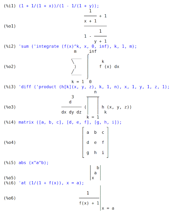
Same expressions, displayed using only ASCII characters (
display2d_unicodeequal tofalse), shown as an image: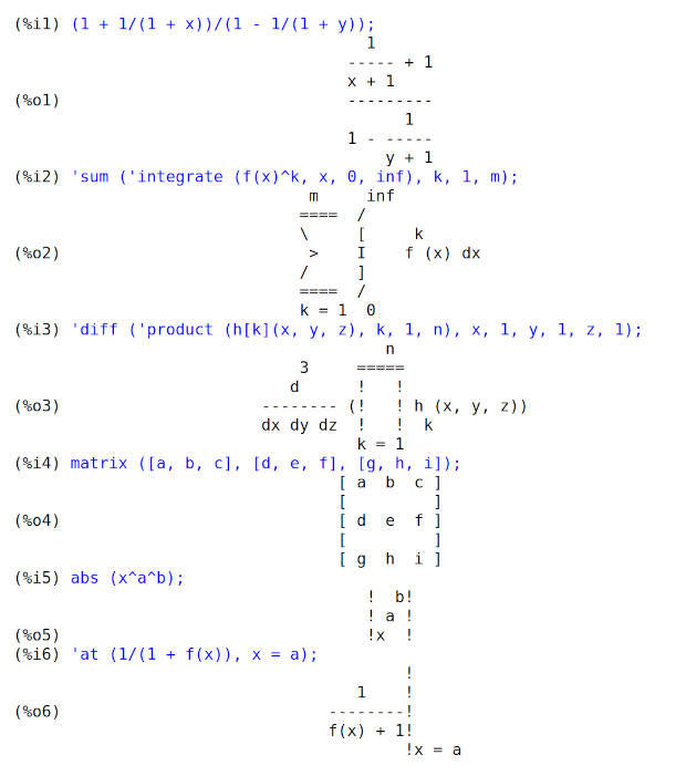
Footnotes:
[1] https://en.wikipedia.org/wiki/Box-drawing_character
Categories: Display flags and variables ·
- Function: dispterms (expr) 
-
Displays expr in parts one below the other. That is, first the operator of expr is displayed, then each term in a sum, or factor in a product, or part of a more general expression is displayed separately. This is useful if expr is too large to be otherwise displayed. For example if
P1,P2, … are very large expressions then the display program may run out of storage space in trying to displayP1 + P2 + ...all at once. However,dispterms (P1 + P2 + ...)displaysP1, then below itP2, etc. When not usingdispterms, if an exponential expression is too wide to be displayed asA^Bit appears asexpt (A, B)(or asncexpt (A, B)in the case ofA^^B).Example:
(%i1) dispterms(2*a*sin(x)+%e^x); + 2 a sin(x) x %e (%o1) done
Categories: Display functions ·
- Special symbol: expt (a, b) 
- Special symbol: ncexpt (a, b) 
-
If an exponential expression is too wide to be displayed as
a^bit appears asexpt (a, b)(or asncexpt (a, b)in the case ofa^^b).exptandncexptare not recognized in input.
- Option variable: exptdispflag 
Default value:
trueWhen
exptdispflagistrue, Maxima displays expressions with negative exponents using quotients. See also%edispflag.Example:
(%i1) exptdispflag:true; (%o1) true
(%i2) 10^-x; 1 (%o2) --- x 10(%i3) exptdispflag:false; (%o3) false
(%i4) 10^-x; - x (%o4) 10Categories: Expressions · Display flags and variables ·
- Function: grind (expr) 
-
The function
grindprints expr to the console in a form suitable for input to Maxima.grindalways returnsdone.When expr is the name of a function or macro,
grindprints the function or macro definition instead of just the name.See also
string, which returns a string instead of printing its output.grindattempts to print the expression in a manner which makes it slightly easier to read than the output ofstring.grindevaluates its argument.Examples:
(%i1) aa + 1729; (%o1) aa + 1729
(%i2) grind (%); aa+1729$ (%o2) done
(%i3) [aa, 1729, aa + 1729]; (%o3) [aa, 1729, aa + 1729]
(%i4) grind (%); [aa,1729,aa+1729]$ (%o4) done
(%i5) matrix ([aa, 17], [29, bb]); [ aa 17 ] (%o5) [ ] [ 29 bb ](%i6) grind (%); matrix([aa,17],[29,bb])$ (%o6) done
(%i7) set (aa, 17, 29, bb); (%o7) {17, 29, aa, bb}(%i8) grind (%); {17,29,aa,bb}$ (%o8) done(%i9) exp (aa / (bb + 17)^29); aa ----------- 29 (bb + 17) (%o9) %e(%i10) grind (%); %e^(aa/(bb+17)^29)$ (%o10) done
(%i11) expr: expand ((aa + bb)^10); 10 9 2 8 3 7 4 6 (%o11) bb + 10 aa bb + 45 aa bb + 120 aa bb + 210 aa bb 5 5 6 4 7 3 8 2 + 252 aa bb + 210 aa bb + 120 aa bb + 45 aa bb 9 10 + 10 aa bb + aa(%i12) grind (expr); bb^10+10*aa*bb^9+45*aa^2*bb^8+120*aa^3*bb^7+210*aa^4*bb^6 +252*aa^5*bb^5+210*aa^6*bb^4+120*aa^7*bb^3+45*aa^8*bb^2 +10*aa^9*bb+aa^10$ (%o12) done(%i13) string (expr); (%o13) bb^10+10*aa*bb^9+45*aa^2*bb^8+120*aa^3*bb^7+210*aa^4*bb^6\ +252*aa^5*bb^5+210*aa^6*bb^4+120*aa^7*bb^3+45*aa^8*bb^2+10*aa^9*\ bb+aa^10
(%i14) cholesky (A):= block ([n : length (A), L : copymatrix (A), p : makelist (0, i, 1, length (A))], for i thru n do for j : i thru n do (x : L[i, j], x : x - sum (L[j, k] * L[i, k], k, 1, i - 1), if i = j then p[i] : 1 / sqrt(x) else L[j, i] : x * p[i]), for i thru n do L[i, i] : 1 / p[i], for i thru n do for j : i + 1 thru n do L[i, j] : 0, L)$ define: warning: redefining the built-in operator cholesky
(%i15) grind (cholesky); cholesky(A):=block( [n:length(A),L:copymatrix(A), p:makelist(0,i,1,length(A))], for i thru n do (for j from i thru n do (x:L[i,j],x:x-sum(L[j,k]*L[i,k],k,1,i-1), if i = j then p[i]:1/sqrt(x) else L[j,i]:x*p[i])), for i thru n do L[i,i]:1/p[i], for i thru n do (for j from i+1 thru n do L[i,j]:0),L)$ (%o15) done(%i16) string (fundef (cholesky)); (%o16) cholesky(A):=block([n:length(A),L:copymatrix(A),p:makelis\ t(0,i,1,length(A))],for i thru n do (for j from i thru n do (x:L\ [i,j],x:x-sum(L[j,k]*L[i,k],k,1,i-1),if i = j then p[i]:1/sqrt(x\ ) else L[j,i]:x*p[i])),for i thru n do L[i,i]:1/p[i],for i thru \ n do (for j from i+1 thru n do L[i,j]:0),L)
Categories: Display functions ·
- Option variable: grind 
-
When the variable
grindistrue, the output ofstringandstringouthas the same format as that ofgrind; otherwise no attempt is made to specially format the output of those functions. The default value of the variablegrindisfalse.grindcan also be specified as an argument ofplayback. Whengrindis present,playbackprints input expressions in the same format as thegrindfunction. Otherwise, no attempt is made to specially format input expressions.Categories: Display flags and variables ·
- Option variable: ibase 
Default value:
10ibaseis the base for integers read by Maxima.ibasemay be assigned any integer between 2 and 36 (decimal), inclusive. Whenibaseis greater than 10, the numerals comprise the decimal numerals 0 through 9 plus letters of the alphabetA,B,C, …, as needed to makeibasedigits in all. Letters are interpreted as digits only if the first digit is 0 through 9.Uppercase and lowercase letters are not distinguished. The numerals for base 36, the largest acceptable base, comprise 0 through 9 and
AthroughZ.Whatever the value of
ibase, when an integer is terminated by a decimal point, it is interpreted in base 10.See also
obase.Examples:
ibaseless than 10 (for example binary numbers).(%i1) ibase : 2 $
(%i2) obase; (%o2) 10
(%i3) 1111111111111111; (%o3) 65535
ibasegreater than 10. Letters are interpreted as digits only if the first digit is 0 through 9 which means that hexadecimal numbers might need to be prepended by a 0.(%i1) ibase : 16 $
(%i2) obase; (%o2) 10
(%i3) 1000; (%o3) 4096
(%i4) abcd; (%o4) abcd
(%i5) symbolp (abcd); (%o5) true
(%i6) 0abcd; (%o6) 43981
(%i7) symbolp (0abcd); (%o7) false
When an integer is terminated by a decimal point, it is interpreted in base 10.
(%i1) ibase : 36 $
(%i2) obase; (%o2) 10
(%i3) 1234; (%o3) 49360
(%i4) 1234.; (%o4) 1234
Categories: Console interaction ·
- Function: ldisp (expr_1, …, expr_n) 
-
Displays expressions expr_1, …, expr_n to the console as printed output.
ldispassigns an intermediate expression label to each argument and returns the list of labels.See also
disp,display, andldisplay.Examples:
(%i1) e: (a+b)^3; 3 (%o1) (b + a)(%i2) f: expand (e); 3 2 2 3 (%o2) b + 3 a b + 3 a b + a(%i3) ldisp (e, f); 3 (%t3) (b + a) 3 2 2 3 (%t4) b + 3 a b + 3 a b + a (%o4) [%t3, %t4](%i5) %t3; 3 (%o5) (b + a)(%i6) %t4; 3 2 2 3 (%o6) b + 3 a b + 3 a b + aCategories: Display functions ·
- Function: ldisplay (expr_1, …, expr_n) 
-
Displays expressions expr_1, …, expr_n to the console as printed output. Each expression is printed as an equation of the form
lhs = rhsin whichlhsis one of the arguments ofldisplayandrhsis its value. Typically each argument is a variable.ldispassigns an intermediate expression label to each equation and returns the list of labels.See also
display,disp, andldisp.Examples:
(%i1) e: (a+b)^3; 3 (%o1) (b + a)(%i2) f: expand (e); 3 2 2 3 (%o2) b + 3 a b + 3 a b + a(%i3) ldisplay (e, f); 3 (%t3) e = (b + a) 3 2 2 3 (%t4) f = b + 3 a b + 3 a b + a (%o4) [%t3, %t4](%i5) %t3; 3 (%o5) e = (b + a)(%i6) %t4; 3 2 2 3 (%o6) f = b + 3 a b + 3 a b + aCategories: Display functions ·
- Option variable: leftjust 
Default value:
falseWhen
leftjustistrue, equations in 2D-display are drawn left justified rather than centered.See also
display2dto switch between 1D- and 2D-display.Example:
(%i1) expand((x+1)^3); 3 2 (%o1) x + 3 x + 3 x + 1(%i2) leftjust:true$
(%i3) expand((x+1)^3); 3 2 (%o3) x + 3 x + 3 x + 1Categories: Display flags and variables ·
- Option variable: linel 
Default value:
79linelis the assumed width (in characters) of the console display for the purpose of displaying expressions.linelmay be assigned any value by the user, although very small or very large values may be impractical. Text printed by built-in Maxima functions, such as error messages and the output ofdescribe, is not affected bylinel.Categories: Display flags and variables ·
- Option variable: lispdisp 
Default value:
falseWhen
lispdispistrue, Lisp symbols are displayed with a leading question mark?. Otherwise, Lisp symbols are displayed with no leading mark. This has the same effect for 1-d and 2-d display.Examples:
(%i1) lispdisp: false$
(%i2) ?foo + ?bar; (%o2) foo + bar
(%i3) lispdisp: true$
(%i4) ?foo + ?bar; (%o4) ?foo + ?bar
Categories: Display flags and variables ·
- Option variable: negsumdispflag 
Default value:
trueWhen
negsumdispflagistrue,x - ydisplays asx - yinstead of as- y + x. Setting it tofalsecauses the special check in display for the difference of two expressions to not be done. One application is that thusa + %i*banda - %i*bmay both be displayed the same way.Categories: Display flags and variables ·
- Option variable: obase 
Default value:
10obaseis the base for integers displayed by Maxima.obasemay be assigned any integer between 2 and 36 (decimal), inclusive. Whenobaseis greater than 10, the numerals comprise the decimal numerals 0 through 9 plus capital letters of the alphabet A, B, C, …, as needed. A leading 0 digit is displayed if the leading digit is otherwise a letter. The numerals for base 36, the largest acceptable base, comprise 0 through 9, and A through Z.See also
ibase.Examples:
(%i1) obase : 2; (%o1) 10
(%i2) 2^8 - 1; (%o2) 11111111
(%i3) obase : 8; (%o3) 10
(%i4) 8^8 - 1; (%o4) 77777777
(%i5) obase : 16; (%o5) 10
(%i6) 16^8 - 1; (%o6) 0FFFFFFFF
(%i7) obase : 36; (%o7) 10
(%i8) 36^8 - 1; (%o8) 0ZZZZZZZZ
Categories: Display flags and variables · Console interaction ·
- Option variable: pfeformat 
Default value:
falseWhen
pfeformatistrue, a ratio of integers is displayed with the solidus (forward slash) character, and an integer denominatornis displayed as a leading multiplicative term1/n.Examples:
(%i1) pfeformat: false$
(%i2) 2^16/7^3; 65536 (%o2) ----- 343(%i3) (a+b)/8; b + a (%o3) ----- 8(%i4) pfeformat: true$
(%i5) 2^16/7^3; (%o5) 65536/343
(%i6) (a+b)/8; (%o6) (1/8) (b + a)
Categories: Display flags and variables ·
- Option variable: powerdisp 
Default value:
falseWhen
powerdispistrue, a sum is displayed with its terms in order of increasing power. Thus a polynomial is displayed as a truncated power series, with the constant term first and the highest power last.By default, terms of a sum are displayed in order of decreasing power.
Example:
(%i1) powerdisp:true; (%o1) true
(%i2) x^2+x^3+x^4; 2 3 4 (%o2) x + x + x(%i3) powerdisp:false; (%o3) false
(%i4) x^2+x^3+x^4; 4 3 2 (%o4) x + x + xCategories: Display flags and variables ·
- Function: print (expr_1, …, expr_n) 
-
Evaluates and displays expr_1, …, expr_n one after another, from left to right, starting at the left edge of the console display.
The value returned by
printis the value of its last argument.printdoes not generate intermediate expression labels.See also
display,disp,ldisplay, andldisp. Those functions display one expression per line, whileprintattempts to display two or more expressions per line.To display the contents of a file, see
printfile.Examples:
(%i1) r: print ("(a+b)^3 is", expand ((a+b)^3), "log (a^10/b) is", radcan (log (a^10/b)))$ 3 2 2 3 (a+b)^3 is b + 3 a b + 3 a b + a log (a^10/b) is 10 log(a) - log(b)(%i2) r; (%o2) 10 log(a) - log(b)
(%i3) disp ("(a+b)^3 is", expand ((a+b)^3), "log (a^10/b) is", radcan (log (a^10/b)))$ (a+b)^3 is 3 2 2 3 b + 3 a b + 3 a b + a log (a^10/b) is 10 log(a) - log(b)Categories: Display functions ·
- Option variable: sqrtdispflag 
Default value:
trueWhen
sqrtdispflagisfalse, causessqrtto display with exponent 1/2.Categories: Mathematical functions · Display flags and variables ·
- Option variable: stardisp 
Default value:
falseWhen
stardispistrue, multiplication is displayed with an asterisk*between operands.Categories: Display flags and variables ·
- Option variable: ttyoff 
Default value:
falseWhen
ttyoffistrue, output expressions are not displayed. Output expressions are still computed and assigned labels. Seelabels.Text printed by built-in Maxima functions, such as error messages and the output of
describe, is not affected byttyoff.Categories: Display flags and variables ·
Next: Expressions, Previous: Command Line [Contents][Index]
7 Data Types and Structures
Next: Strings, Previous: Data Types and Structures, Up: Data Types and Structures [Contents][Index]
7.1 Numbers
Next: Functions and Variables for Numbers, Previous: Numbers, Up: Numbers [Contents][Index]
7.1.1 Introduction to Numbers
Complex numbers
A complex expression is specified in Maxima by adding the real part of the
expression to %i times the imaginary part. Thus the roots of the
equation x^2 - 4*x + 13 = 0 are 2 + 3*%i and 2 - 3*%i.
Note that simplification of products of complex expressions can be effected by
expanding the product. Simplification of quotients, roots, and other functions
of complex expressions can usually be accomplished by using the realpart,
imagpart, rectform, polarform, abs, carg
functions.
Previous: Introduction to Numbers, Up: Numbers [Contents][Index]
7.1.2 Functions and Variables for Numbers
- Function: bfloat (expr) 
-
bfloatreplaces integers, rationals, floating point numbers, and some symbolic constants in expr with bigfloat (variable-precision floating point) numbers.The constants
%e,%gamma,%phi, and%piare replaced by a numerical approximation. However,%ein%e^xis not replaced by a numeric value unlessbfloat(x)is a number.bfloatalso causes numerical evaluation of some built-in functions, namely trigonometric functions, exponential functions,abs, andlog.The number of significant digits in the resulting bigfloats is specified by the global variable
fpprec. Bigfloats already present in expr are replaced with values which have precision specified by the current value offpprec.When
float2bfisfalse, a warning message is printed when a floating point number is replaced by a bigfloat number with less precision.Examples:
bfloatreplaces integers, rationals, floating point numbers, and some symbolic constants in expr with bigfloat numbers.(%i1) bfloat([123, 17/29, 1.75]); (%o1) [1.23b2, 5.862068965517241b-1, 1.75b0] (%i2) bfloat([%e, %gamma, %phi, %pi]); (%o2) [2.718281828459045b0, 5.772156649015329b-1, 1.618033988749895b0, 3.141592653589793b0] (%i3) bfloat((f(123) + g(h(17/29)))/(x + %gamma)); 1.0b0 (g(h(5.862068965517241b-1)) + f(1.23b2)) (%o3) ---------------------------------------------- x + 5.772156649015329b-1bfloatalso causes numerical evaluation of some built-in functions.(%i1) bfloat(sin(17/29)); (%o1) 5.532051841609784b-1 (%i2) bfloat(exp(%pi)); (%o2) 2.314069263277927b1 (%i3) bfloat(abs(-%gamma)); (%o3) 5.772156649015329b-1 (%i4) bfloat(log(%phi)); (%o4) 4.812118250596035b-1
Categories: Numerical evaluation ·
- Function: bfloatp (expr) 
-
Returns
trueif expr is a bigfloat number, otherwisefalse.Categories: Numerical evaluation · Predicate functions ·
- Option variable: bftorat 
Default value:
falsebftoratcontrols the conversion of bfloats to rational numbers. Whenbftoratisfalse,ratepsilonwill be used to control the conversion (this results in relatively small rational numbers). Whenbftoratistrue, the rational number generated will accurately represent the bfloat.Note:
bftorathas no effect on the transformation to rational numbers with the functionrationalize.Example:
(%i1) ratepsilon:1e-4; (%o1) 1.0e-4 (%i2) rat(bfloat(11111/111111)), bftorat:false; `rat' replaced 9.99990999991B-2 by 1/10 = 1.0B-1 1 (%o2)/R/ -- 10 (%i3) rat(bfloat(11111/111111)), bftorat:true; `rat' replaced 9.99990999991B-2 by 11111/111111 = 9.99990999991B-2 11111 (%o3)/R/ ------ 111111Categories: Numerical evaluation ·
- Option variable: bftrunc 
Default value:
truebftrunccauses trailing zeroes in non-zero bigfloat numbers not to be displayed. Thus, ifbftruncisfalse,bfloat (1)displays as1.000000000000000B0. Otherwise, this is displayed as1.0B0.Categories: Numerical evaluation ·
- Function: bigfloat_bits () 
Returns the number of bits of precision in a bigfloat number. This value depends, of course, on the value of
fpprec.(%i1) fpprec:16; (%o1) 16 (%i2) bigfloat_bits(); (%o2) 56 (%i3) fpprec:32; (%o3) 32 (%i4) bigfloat_bits(); (%o4) 109
Categories: Numerical evaluation ·
- Function: bigfloat_eps () 
Returns the smallest bigfloat value,
eps, such that1+epsis not equal to 1. The value depends onfpprec, of course.(%i1) fpprec:16; (%o1) 16 (%i2) bigfloat_eps(); (%o2) 1.387778780781446b-17 (%i3) fpprec:32; (%o3) 32 (%i4) bigfloat_eps(); (%o4) 1.5407439555097886824447823540679b-33
Categories: Numerical evaluation ·
- Function: decode_float (f) 
decode_floattakes a float f and returns a list of three values that characterizes f, which must be either afloatorbfloat. The first value has the same type as f, but is a number in the range[1, 2). The second value is an exponent. The third value is a float of the same type as f and has the value of 1 if f is greater than or equal to 0; otherwise, -1.If the returned list is
[mantissa, expo, sign], thenscale_float(mantissa, exp)*signis identical to f.(%i1) decode_float(4e0); (%o1) [1.0, 2, 1.0] (%i2) decode_float(4b0); (%o2) [1.0b0, 2, 1.0b0] (%i3) decode_float(%pi); decode_float is only defined for floats and bfloats: %pi -- an error. To debug this try: debugmode(true); (%i4) decode_float(float(%pi)); (%o4) [1.570796326794897, 1, 1.0] (%i5) decode_float(1.1e-5); (%o5) [1.441792, - 17, 1.0] (%i6) %[1]*2^%[2]; (%o6) 1.1e-5
This is a relatively simple interface to Common Lisp decode_float. However we return a signficand in the range
[1,2)instead of[0.5, 1). The former matches IEEE-754. Of course, this is extended to support bfloats.Categories: Numerical evaluation ·
- Function: evenp (expr) 
-
Returns
trueif expr is a literal even integer, otherwisefalse.evenpreturnsfalseif expr is a symbol, even if expr is declaredeven.Categories: Predicate functions ·
- Function: float (expr) 
-
Converts integers, rational numbers and bigfloats in expr to floating point numbers. It is also an
evflag,floatcauses non-integral rational numbers and bigfloat numbers to be converted to floating point.Categories: Numerical evaluation · Evaluation flags ·
- Option variable: float2bf 
Default value:
trueWhen
float2bfisfalse, a warning message is printed when a floating point number is replaced by a bigfloat number with less precision.Categories: Numerical evaluation ·
- Function: float_bits () 
Returns the number of bits of precision of a floating-point number.
Categories: Numerical evaluation ·
- Function: float_eps () 
Returns the smallest floating-point value,
eps, such that1+epsis not equal to 1.Categories: Numerical evaluation ·
- Function: float_precision (f) 
Returns the number of bits of precision of a floating-point number, which can be either a float or bigfloat. This is basically the number of bits used to represent the mantissa of a floating-point number. For floats, this is 53 (for IEEE double-floats), but can be less when denormal numbers occur. For bigfloats, this is equal to
fpprec, when converted from digits to bits.Categories: Numerical evaluation ·
- Function: float_sign (f) 
Returns the sign of f. It is +1 or -1 of the same type as f. It is an error if f is not a float or bigfloat. Note that some lisps do not support signed zeros for floating-point numbers. Bigfloats do not support signed zeroes. The examples below assume signed zeroes are supported.
(%i1) float_sign(1.0); (%o1) 1.0 (%i2) float_sign(-5.0); (%o2) - 1.0 (%i3) float_sign(-0.0); (%o3) - 1.0 (%i4) float_sign(1b0); (%o4) 1.0b0 (%i5) float_sign(-5b0); (%o5) - 1.0b0 (%o6) float_sign(-0b0); (%o6) 1.0b0 (%i7) float_sign(%pi); float_sign is only defined for floats and bfloats: %pi -- an error. To debug this try: debugmode(true);
- Function: float_infinity_p (x) 
-
Returns
trueif x is floating point positive infinity or floating point negative infinity, and returnsfalsefor all other arguments; arguments which are not numbers are allowed, andfloat_infinity_preturnsfalsefor all such arguments.Positive and negative floating point infinity may be distinguished by
sign, which returnsposfor positive infinity andnegfor negative infinity.float_infinity_pis defined whether or not the Lisp implementation supports float infinity. When float infinity does not exist in the Lisp implementation’s number system,float_infinity_preturnsfalsefor all arguments.A Lisp implementation may support more than one precision of floating point numbers.
float_infinity_ponly recognizes double precision floating point infinity, and not any other precision.Categories: Numerical evaluation · Predicate functions ·
- Function: float_nan_p (x) 
-
Returns
trueif x is a floating point not-a-number (NaN) value, and returnsfalsefor all other arguments; arguments which are not numbers are allowed, andfloat_nan_preturnsfalsefor all such arguments.float_nan_pis defined whether or not the Lisp implementation supports floating point not-a-number values. When floating point not-a-number does not exist in the Lisp implementation’s number system,float_nan_preturnsfalsefor all arguments.A Lisp implementation may support more than one precision of floating point numbers.
float_nan_ponly recognizes double precision floating point not-a-number, and not any other precision.Categories: Numerical evaluation · Predicate functions ·
- Function: floatnump (expr) 
-
Returns
trueif expr is a floating point number, otherwisefalse.Categories: Numerical evaluation · Predicate functions ·
- Option variable: fpprec 
Default value: 16
fpprecis the number of significant digits for arithmetic on bigfloat numbers.fpprecdoes not affect computations on ordinary floating point numbers.See also
bfloatandfpprintprec.Categories: Numerical evaluation ·
- Option variable: fpprintprec 
Default value: 0
fpprintprecis the number of digits to print when printing an ordinary float or bigfloat number.For ordinary floating point numbers, when
fpprintprechas a value between 2 and 16 (inclusive), the number of digits printed is equal tofpprintprec. Otherwise,fpprintprecis 0, or greater than 16, and the number is printed "readably": that is, it is printed with sufficient digits to exactly reconstruct the number on input.For bigfloat numbers, when
fpprintprechas a value between 2 andfpprec(inclusive), the number of digits printed is equal tofpprintprec. Otherwise,fpprintprecis 0, or greater thanfpprec, and the number of digits printed is equal tofpprec.For both ordinary floats and bigfloats, trailing zero digits are suppressed. The actual number of digits printed is less than
fpprintprecif there are trailing zero digits.fpprintpreccannot be 1.Categories: Numerical evaluation · Display flags and variables ·
- Function: integerp (expr) 
-
Returns
trueif expr is a literal numeric integer, otherwisefalse.integerpreturnsfalseif expr is a symbol, even if expr is declaredinteger.Examples:
(%i1) integerp (0); (%o1) true (%i2) integerp (1); (%o2) true (%i3) integerp (-17); (%o3) true (%i4) integerp (0.0); (%o4) false (%i5) integerp (1.0); (%o5) false (%i6) integerp (%pi); (%o6) false (%i7) integerp (n); (%o7) false (%i8) declare (n, integer); (%o8) done (%i9) integerp (n); (%o9) false
Categories: Predicate functions ·
- Function: integer_decode_float (f) 
integer_decode_floattakes a float f and returns a list of three values that characterizes f, which must be either afloatorbfloat. The first value is an integer. The second value is an exponent. The third value is 1 if f is positive or zero; otherwise, -1.If the returned list is
[mantissa, expo, sign], thenscale_float(fl(mantissa), expo)*signis identical to f. Here,flis eitherfloatorbfloatdepending on whether f is afloator abfloat.(%i1) integer_decode_float(4.0); (%o1) [4503599627370496, - 50, 1] (%i2) integer_decode_float(4b0); (%o2) [36028797018963968, - 53, 1] (%i3) scale_float(float(%o1[1]), %o1[2]); (%o3) 4.0 (%i4) scale_float(bfloat(%o2[1]), %o2[2]); (%o4) 4.0b0 (%i5) integer_decode_float(4); decode_float is only defined for floats and bfloats: 4 -- an error. To debug this try: debugmode(true); (%i6) integer_decode_float(1e-7); (%o6) [7555786372591432, - 76, 1] (%i7) integer_decode_float(1b-7); (%o7) [60446290980731459, - 79, 1] (%i8) scale_float(float(%o6[1]), %o6[2]); (%o8) 1.0e-7
For lisps that support denormal numbers, we have the following results.
(%i1) integer_decode_float(least_positive_float); (%o1) [1, - 1074, 1] (%i2) integer_decode_float(100*least_positive_float); (%o2) [100, - 1074, 1] (%i3) integer_decode_float(least_positive_normalized_float); (%o3) [4503599627370496, - 1074, 1]
The number of bits in the integer part decreases as the denormal number decreases. Bfloat numbers do not have denormals because the exponent is not bounded.
This is a relatively simple interface to Common Lisp integer_decode_float. However, the integer part can vary depending on the Lisp implementation; we return the same value, independent of the Lisp implementation. Of course, this is extended to support bfloats.
Categories: Numerical evaluation ·
- Function: is_power_of_two (n) 
is_power_to_tworeturnstrueif n is a power of two andfalseotherwise. n may be an integer, a rational, a float, or a big float.Some examples:
(%i1) is_power_of_two(0); (%o1) false (%i2) is_power_of_two(4); (%o2) true (%i3) is_power_of_two(355/113); (%o3) false (%i4) is_power_of_two(1/32); (%o4) true (%i5) is_power_of_two(1048576); (%o5) true (%i6) is_power_of_two(1048575); (%o6) false (%i7) is_power_of_two(0.0); (%o7) false (%i8) is_power_of_two(1048576.0); (%o8) true (%i9) is_power_of_two(1048575.0); (%o9) false (%i10) is_power_of_two(1/256.0); (%o10) true (%i11) is_power_of_two(0b0); (%o11) false (%i12) is_power_of_two(1048576b0); (%o12) true (%i13) is_power_of_two(1048575b0); (%o13) false (%i14) is_power_of_two(1/256b0); (%o14) true
Categories: Predicate functions ·
- Option variable: m1pbranch 
Default value:
falsem1pbranchis the principal branch for-1to a power. Quantities such as(-1)^(1/3)(that is, an "odd" rational exponent) and(-1)^(1/4)(that is, an "even" rational exponent) are handled as follows:domain:real (-1)^(1/3): -1 (-1)^(1/4): (-1)^(1/4) domain:complex m1pbranch:false m1pbranch:true (-1)^(1/3) 1/2+%i*sqrt(3)/2 (-1)^(1/4) sqrt(2)/2+%i*sqrt(2)/2Categories: Expressions · Global flags ·
- Function: nonnegintegerp (n) 
-
Return
trueif and only ifn >= 0and n is an integer.Categories: Predicate functions ·
- Function: numberp (expr) 
-
Returns
trueif expr is a literal integer, rational number, floating point number, or bigfloat, otherwisefalse.numberpreturnsfalseif expr is a symbol, even if expr is a symbolic number such as%pior%i, or declared to beeven,odd,integer,rational,irrational,real,imaginary, orcomplex.Examples:
(%i1) numberp (42); (%o1) true (%i2) numberp (-13/19); (%o2) true (%i3) numberp (3.14159); (%o3) true (%i4) numberp (-1729b-4); (%o4) true (%i5) map (numberp, [%e, %pi, %i, %phi, inf, minf]); (%o5) [false, false, false, false, false, false] (%i6) declare (a, even, b, odd, c, integer, d, rational, e, irrational, f, real, g, imaginary, h, complex); (%o6) done (%i7) map (numberp, [a, b, c, d, e, f, g, h]); (%o7) [false, false, false, false, false, false, false, false]Categories: Predicate functions ·
- Option variable: numer 
-
numercauses some mathematical functions (including exponentiation) with numerical arguments to be evaluated in floating point. It causes variables inexprwhich have been given numerals to be replaced by their values. It also sets thefloatswitch on.See also
%enumer.Examples:
(%i1) [sqrt(2), sin(1), 1/(1+sqrt(3))]; 1 (%o1) [sqrt(2), sin(1), -----------] sqrt(3) + 1(%i2) [sqrt(2), sin(1), 1/(1+sqrt(3))],numer; (%o2) [1.414213562373095, 0.8414709848078965, 0.3660254037844387]
Categories: Numerical evaluation · Evaluation flags ·
- Option variable: numer_pbranch 
Default value:
falseThe option variable
numer_pbranchcontrols the numerical evaluation of the power of a negative integer, rational, or floating point number. Whennumer_pbranchistrueand the exponent is a floating point number or the option variablenumeristruetoo, Maxima evaluates the numerical result using the principal branch. Otherwise a simplified, but not an evaluated result is returned.Examples:
(%i1) (-2)^0.75; 0.75 (%o1) (- 2)(%i2) (-2)^0.75,numer_pbranch:true; (%o2) 1.189207115002721 %i - 1.189207115002721
(%i3) (-2)^(3/4); 3/4 3/4 (%o3) (- 1) 2(%i4) (-2)^(3/4),numer; 0.75 (%o4) 1.681792830507429 (- 1)(%i5) (-2)^(3/4),numer,numer_pbranch:true; (%o5) 1.189207115002721 %i - 1.189207115002721
Categories: Numerical evaluation ·
- Function: numerval (x_1, expr_1, …, var_n, expr_n) 
-
Declares the variables
x_1, …, x_n to have numeric values equal toexpr_1, …,expr_n. The numeric value is evaluated and substituted for the variable in any expressions in which the variable occurs if thenumerflag istrue. See alsoev.The expressions
expr_1, …,expr_ncan be any expressions, not necessarily numeric.Categories: Declarations and inferences · Numerical evaluation ·
- Function: oddp (expr) 
-
Returns
trueif expr is a literal odd integer, otherwisefalse.oddpreturnsfalseif expr is a symbol, even if expr is declaredodd.Categories: Predicate functions ·
- Option variable: ratepsilon 
Default value:
2.0e-15ratepsilonis the tolerance used in the conversion of floating point numbers to rational numbers, when the option variablebftorathas the valuefalse. Seebftoratfor an example.Categories: Numerical evaluation · Rational expressions ·
- Function: rationalize (expr) 
-
Convert all double floats and big floats in the Maxima expression expr to their exact rational equivalents. If you are not familiar with the binary representation of floating point numbers, you might be surprised that
rationalize (0.1)does not equal 1/10. This behavior isn’t special to Maxima – the number 1/10 has a repeating, not a terminating, binary representation.(%i1) rationalize (0.5); 1 (%o1) - 2(%i2) rationalize (0.1); 3602879701896397 (%o2) ----------------- 36028797018963968(%i3) fpprec : 5$
(%i4) rationalize (0.1b0); 209715 (%o4) ------- 2097152(%i5) fpprec : 20$
(%i6) rationalize (0.1b0); 236118324143482260685 (%o6) ---------------------- 2361183241434822606848(%i7) rationalize (sin (0.1*x + 5.6)); 3602879701896397 x 3152519739159347 (%o7) sin(------------------ + ----------------) 36028797018963968 562949953421312Categories: Numerical evaluation ·
- Function: ratnump (expr) 
-
Returns
trueif expr is a literal integer or ratio of literal integers, otherwisefalse.Categories: Predicate functions · Rational expressions ·
- Function: scale_float (f, n) 
scale_floatscales the float f by the value2^n. This is done carefully so that no round-off every occurs. If f is a float, then it is possible to underflow to 0 or overflow, depending on the value of f and n. Bigfloats cannot underflow or overflow.(%i1) scale_float(2d0, 2); (%o1) 8.0 (%i2) scale_float(2d0, -2); (%o2) 0.5 (%i3) scale_float(-2d0, -10); (%o3) - 0.001953125 (%i4) scale_float(1d0, -2000); (%o4) 0.0 (%i5) scale_float(2b0, 2); (%o5) 8.0b0 (%i6) scale_float(1b0, -2000); (%o6) 8.709809816217217b-603 (%i7) scale_float(1, 5); scale_float: first arg must be a float or bfloat: 1 -- an error. To debug this try: debugmode(true); (%i8) scale_float(1.0, n); scale_float: second arg must be an integer: n -- an error. To debug this try: debugmode(true);
This is a relatively simple interface to Common Lisp scale_float. Of course, this is extended to support bfloats.
- Function: unit_in_last_place (n) 
-
unit_in_last_placereturns a value that is the gap between n and the nearest other number. See, for example, Kahan, FOOTNOTE 1.unit_in_last_placesupports rational numbers, floating-point numbers and bigfloat numbers. For integer, the result is always 1, and for rational numbers the result is always 0.The examples below assume IEEE-754 arithmetic that supports denormal numbers. Some lisps like Clisp do not have denormal numbers.
(%i1) unit_in_last_place(0); (%o1) 1 (%i2) unit_in_last_place(-123); (%o2) 1 (%i3) unit_in_last_place(2/3); (%o3) 0 (%i4) unit_in_last_place(355/113); (%o4) 0 (%i5) unit_in_last_place(0b0); (%o5) 0.0b0 (%i6) unit_in_last_place(0.0); (%o6) 4.940656458412465e-324 (%i7) unit_in_last_place(1.0); (%o7) 1.110223024625157e-16 (%i8) unit_in_last_place(1b0); (%o8) 1.387778780781446b-17 (%i9) unit_in_last_place(100.0); (%o9) 1.4210854715202e-14 (%i10) unit_in_last_place(100b0); (%o10) 1.77635683940025b-15 (%i11) fpprec:32; (%o11) 32 (%i12) unit_in_last_place(1b0); (%o12) 1.5407439555097886824447823540679b-33 (%i13) unit_in_last_place(100b0); (%o13) 1.972152263052529513529321413207b-31
Categories: Numerical evaluation ·
Next: Constants, Previous: Numbers, Up: Data Types and Structures [Contents][Index]
7.2 Strings
Next: Functions and Variables for Strings, Previous: Strings, Up: Strings [Contents][Index]
7.2.1 Introduction to Strings
Strings (quoted character sequences) are enclosed in double quote marks "
for input, and displayed with or without the quote marks, depending on the
global variable stringdisp.
Strings may contain any characters, including embedded tab, newline, and
carriage return characters. The sequence \" is recognized as a literal
double quote, and \\ as a literal backslash. When backslash appears at
the end of a line, the backslash and the line termination (either newline or
carriage return and newline) are ignored, so that the string continues with the
next line. No other special combinations of backslash with another character
are recognized; when backslash appears before any character other than ",
\, or a line termination, the backslash is ignored. There is no way to
represent a special character (such as tab, newline, or carriage return)
except by embedding the literal character in the string.
There is no character type in Maxima; a single character is represented as a one-character string.
The stringproc add-on package contains many functions for working with
strings.
Examples:
(%i1) s_1 : "This is a string."; (%o1) This is a string.
(%i2) s_2 : "Embedded \"double quotes\" and backslash \\ characters."; (%o2) Embedded "double quotes" and backslash \ characters.
(%i3) s_3 : "Embedded line termination in this string."; (%o3) Embedded line termination in this string.
(%i4) s_4 : "Ignore the \ line termination \ characters in \ this string."; (%o4) Ignore the line termination characters in this string.
(%i5) stringdisp : false; (%o5) false
(%i6) s_1; (%o6) This is a string.
(%i7) stringdisp : true; (%o7) true
(%i8) s_1; (%o8) "This is a string."
Previous: Introduction to Strings, Up: Strings [Contents][Index]
7.2.2 Functions and Variables for Strings
- Function: concat (arg_1, arg_2, …) 
-
Concatenates its arguments. The arguments must evaluate to atoms. The return value is a symbol if the first argument is a symbol and a string otherwise.
concatevaluates its arguments. The single quote'prevents evaluation.See also
sconcat, that works on non-atoms, too,simplode,stringandeval_string. For complex string conversions see alsoprintf.(%i1) y: 7$ (%i2) z: 88$ (%i3) concat (y, z/2); (%o3) 744 (%i4) concat ('y, z/2); (%o4) y44A symbol constructed by
concatmay be assigned a value and appear in expressions. The::(double colon) assignment operator evaluates its left-hand side.(%i5) a: concat ('y, z/2); (%o5) y44 (%i6) a:: 123; (%o6) 123 (%i7) y44; (%o7) 123 (%i8) b^a; y44 (%o8) b (%i9) %, numer; 123 (%o9) bNote that although
concat (1, 2)looks like a number, it is a string.(%i10) concat (1, 2) + 3; (%o10) 12 + 3
Categories: Expressions · Strings ·
- Function: sconcat (arg_1, arg_2, …) 
-
Concatenates its arguments into a string. Unlike
concat, the arguments do not need to be atoms.See also
concat,simplode,stringandeval_string. For complex string conversions see alsoprintf.(%i1) sconcat ("xx[", 3, "]:", expand ((x+y)^3)); (%o1) xx[3]:y^3+3*x*y^2+3*x^2*y+x^3Another purpose for
sconcatis to convert arbitrary objects to strings.(%i1) sconcat (x); (%o1) x
(%i2) stringp(%); (%o2) true
Categories: Expressions · Strings ·
- Function: string (expr) 
-
Converts
exprto Maxima’s linear notation just as if it had been typed in.The return value of
stringis a string, and thus it cannot be used in a computation.See also
concat,sconcat,simplodeandeval_string.Categories: Strings ·
- Option variable: stringdisp 
Default value:
falseWhen
stringdispistrue, strings are displayed enclosed in double quote marks. Otherwise, quote marks are not displayed.stringdispis alwaystruewhen displaying a function definition.Examples:
(%i1) stringdisp: false$
(%i2) "This is an example string."; (%o2) This is an example string.
(%i3) foo () := print ("This is a string in a function definition."); (%o3) foo() := print("This is a string in a function definition.")(%i4) stringdisp: true$
(%i5) "This is an example string."; (%o5) "This is an example string."
Categories: Display flags and variables ·
Next: Lists, Previous: Strings, Up: Data Types and Structures [Contents][Index]
7.3 Constants
7.3.1 Functions and Variables for Constants
- Constant: %catalan 
-
%catalanrepresents Catalan’s constant, G, defined by $$ G = \sum_{n=0}^\infty {(-1)^n\over (2n+1)^2} $$(It is also sometimes denoted by C).
The numeric value of
%catalanis approximately 0.915965594177219. (See DLMF 25.11.E40).Categories: Constants ·
- Constant: %e 
-
%erepresents the base of the natural logarithm, also known as Euler’s number. The numeric value of%eis the double-precision floating-point value 2.718281828459045d0. (See A&S eqn 4.1.16, A&S 4.1.17.)Categories: Constants ·
- Constant: false 
-
falserepresents the Boolean constant of the same name. Maxima implementsfalseby the valueNILin Lisp.Categories: Constants ·
- Constant: %gamma 
-
The Euler-Mascheroni constant, 0.5772156649015329.... It is defined by (A&S eqn 6.1.3 and DLMF 5.2.ii) $$ \gamma = \lim_{n \rightarrow \infty} \left(\sum_{k=1}^n {1\over k} - \log n\right) $$
Categories: Constants ·
- Constant: ind 
-
indrepresents a bounded, indefinite result.See also
limit.Example:
(%i1) limit (sin(1/x), x, 0); (%o1) ind
Categories: Constants ·
- Constant: least_negative_float 
The least negative floating-point number in Maxima. That is, the negative floating-point number closest to 0. It is approximately -4.94065e-324, when denormal numbers are supported. Otherwise it is the same as
least_negative_normalized_float.Categories: Constants ·
- Constant: least_negative_normalized_float 
The least negative normalized floating-point number in Maxima. That is, the negative normalized floating-point number closest to 0. It is approximately -2.22507e-308.
Categories: Constants ·
- Constant: least_positive_float 
The least positive floating-point number in Maxima. That is, the positive floating-point number closest to 0. It is approximately 4.94065e-324, when denormal numbers are supported. Otherwise it is the same as
least_positive_normalized_float.Categories: Constants ·
- Constant: least_positive_normalized_float 
The least positive normalized floating-point number in Maxima. That is, the positive normalized floating-point number closest to 0. It is approximately 2.22507e-308.
Categories: Constants ·
- Constant: most_negative_float 
The most negative floating-point number in Maxima. It is approximately -1.79769e+308.
Categories: Constants ·
- Constant: most_positive_float 
The most positive floating-point number in Maxima. It is approximately 1.797693e+308.
Categories: Constants ·
- Constant: %phi 
-
%phirepresents the so-called golden mean, \((1+\sqrt{5})/2.\) The numeric value of%phiis the double-precision floating-point value 1.618033988749895d0.fibtophiexpresses Fibonacci numbersfib(n)in terms of%phi.By default, Maxima does not know the algebraic properties of
%phi. After evaluatingtellrat(%phi^2 - %phi - 1)andalgebraic: true,ratsimpcan simplify some expressions containing%phi.Examples:
fibtophiexpresses Fibonacci numbersfib(n)in terms of%phi.(%i1) fibtophi (fib (n)); n n %phi - (1 - %phi) (%o1) ------------------- 2 %phi - 1(%i2) fib (n-1) + fib (n) - fib (n+1); (%o2) - fib(n + 1) + fib(n) + fib(n - 1)
(%i3) fibtophi (%); n + 1 n + 1 n n %phi - (1 - %phi) %phi - (1 - %phi) (%o3) - --------------------------- + ------------------- 2 %phi - 1 2 %phi - 1 n - 1 n - 1 %phi - (1 - %phi) + --------------------------- 2 %phi - 1(%i4) ratsimp (%); (%o4) 0
By default, Maxima does not know the algebraic properties of
%phi. After evaluatingtellrat (%phi^2 - %phi - 1)andalgebraic: true,ratsimpcan simplify some expressions containing%phi.(%i1) e : expand ((%phi^2 - %phi - 1) * (A + 1)); 2 2 (%o1) %phi A - %phi A - A + %phi - %phi - 1(%i2) ratsimp (e); 2 2 (%o2) (%phi - %phi - 1) A + %phi - %phi - 1(%i3) tellrat (%phi^2 - %phi - 1); 2 (%o3) [%phi - %phi - 1](%i4) algebraic : true; (%o4) true
(%i5) ratsimp (e); (%o5) 0
Categories: Constants ·
- Constant: %pi 
-
%pirepresents the ratio of the perimeter of a circle to its diameter. The numeric value of%piis the double-precision floating-point value 3.141592653589793d0.Categories: Constants ·
- Constant: true 
-
truerepresents the Boolean constant of the same name. Maxima implementstrueby the valueTin Lisp.Categories: Constants ·
- Constant: und 
-
undrepresents an undefined result.See also
limit.Example:
(%i1) limit (x*sin(x), x, inf); (%o1) und
Categories: Constants ·
- Constant: zeroa 
-
zeroarepresents an infinitesimal above zero.zeroacan be used in expressions.limitsimplifies expressions which contain infinitesimals.Example:
limitsimplifies expressions which contain infinitesimals:(%i1) limit(zeroa); (%o1) 0
(%i2) limit(zeroa+x); (%o2) x
Categories: Constants ·
- Constant: zerob 
-
zerobrepresents an infinitesimal below zero.zerobcan be used in expressions.limitsimplifies expressions which contain infinitesimals.Categories: Constants ·
Next: Arrays, Previous: Constants, Up: Data Types and Structures [Contents][Index]
7.4 Lists
Next: Functions and Variables for Lists, Previous: Lists, Up: Lists [Contents][Index]
7.4.1 Introduction to Lists
Lists are the basic building block for Maxima and Lisp. All data types
other than arrays, hashed arrays and numbers are represented as Lisp lists,
These Lisp lists have the form
((MPLUS) $A 2)
to indicate an expression a+2. At Maxima level one would see
the infix notation a+2. Maxima also has lists which are printed
as
[1, 2, 7, x+y]
for a list with 4 elements. Internally this corresponds to a Lisp list of the form
((MLIST) 1 2 7 ((MPLUS) $X $Y))
The flag which denotes the type field of the Maxima expression is a list itself, since after it has been through the simplifier the list would become
((MLIST SIMP) 1 2 7 ((MPLUS SIMP) $X $Y))
Next: Performance considerations for Lists, Previous: Introduction to Lists, Up: Lists [Contents][Index]
7.4.2 Functions and Variables for Lists
- Operator: [ 
- Operator: ] 
-
[and]mark the beginning and end, respectively, of a list.[and]also enclose the subscripts of a list, array,hashed array, ormemoizing function. Note that other than for arrays accessing thenth element of a list may need an amount of time that is roughly proportional ton, See Performance considerations for Lists.Note that if an element of a subscripted variable is written to before a list or an array of this name is declared a
hashed array(see Arrays) is created, not a list.Examples:
(%i1) x: [a, b, c]; (%o1) [a, b, c]
(%i2) x[3]; (%o2) c
(%i3) array (y, fixnum, 3); (%o3) y
(%i4) y[2]: %pi; (%o4) %pi
(%i5) y[2]; (%o5) %pi
(%i6) z['foo]: 'bar; (%o6) bar
(%i7) z['foo]; (%o7) bar
(%i8) g[k] := 1/(k^2+1); 1 (%o8) g := ------ k 2 k + 1(%i9) g[10]; 1 (%o9) --- 101
- Function: append (list_1, …, list_n) 
-
Returns a single list of the elements of list_1 followed by the elements of list_2, …
appendalso works on general expressions, e.g.append (f(a,b), f(c,d,e));yieldsf(a,b,c,d,e).See also
addrow,addcolandjoin.Do
example(append);for an example.Categories: Lists · Expressions ·
- Function: assoc
assoc (key, e, default)
assoc (key, e) ¶ -
assocsearches for key as the first part of an argument of e and returns the second part of the first match, if any.key may be any expression. e must be a nonatomic expression, and every argument of e must have exactly two parts.
assocreturns the second part of the first matching argument of e. Matches are determined byis(key = first(a))where a is an argument of e.If there are two or more matches, only the first is returned. If there are no matches, default is returned, if specified. Otherwise,
falseis returned.Examples:
key may be any expression. e must be a nonatomic expression, and every argument of e must have exactly two parts.
assocreturns the second part of the first matching argument of e.(%i1) assoc (f(x), foo(g(x) = y, f(x) = z + 1, h(x) = 2*u)); (%o1) z + 1
If there are two or more matches, only the first is returned.
(%i1) assoc (yy, [xx = 111, yy = 222, yy = 333, yy = 444]); (%o1) 222
If there are no matches, default is returned, if specified. Otherwise,
falseis returned.(%i1) assoc (abc, [[x, 111], [y, 222], [z, 333]], none); (%o1) none
(%i2) assoc (abc, [[x, 111], [y, 222], [z, 333]]); (%o2) false
Categories: Lists · Expressions ·
- Function: cons
cons (expr, list)
cons (expr_1, expr_2) ¶ -
cons (expr, list)returns a new list constructed of the element expr as its first element, followed by the elements of list. This is analogous to the Lisp language construction operation "cons".The Maxima function
conscan also be used where the second argument is other than a list and this might be useful. In this case,cons (expr_1, expr_2)returns an expression with same operator as expr_2 but with argumentcons(expr_1, args(expr_2)). Examples:(%i1) cons(a,[b,c,d]); (%o1) [a, b, c, d]
(%i2) cons(a,f(b,c,d)); (%o2) f(a, b, c, d)
In general,
consapplied to a nonlist doesn’t make sense. For instance,cons(a,b^c)results in an illegal expression, since ’^’ cannot take three arguments.When
inflagis true,consoperates on the internal structure of an expression, otherwiseconsoperates on the displayed form. Especially wheninflagis true,consapplied to a nonlist sometimes gives a surprising result; for example(%i1) cons(a,-a), inflag : true; 2 (%o1) - a(%i2) cons(a,-a), inflag : false; (%o2) 0
Categories: Lists · Expressions ·
- Function: create_list (form, x_1, list_1, …, x_n, list_n) 
-
Create a list by evaluating form with x_1 bound to each element of list_1, and for each such binding bind x_2 to each element of list_2, … The number of elements in the result will be the product of the number of elements in each list. Each variable x_i must actually be a symbol – it will not be evaluated. The list arguments will be evaluated once at the beginning of the iteration.
(%i1) create_list (x^i, i, [1, 3, 7]); 3 7 (%o1) [x, x , x ]With a double iteration:
(%i1) create_list ([i, j], i, [a, b], j, [e, f, h]); (%o1) [[a, e], [a, f], [a, h], [b, e], [b, f], [b, h]]
Instead of list_i two args may be supplied each of which should evaluate to a number. These will be the inclusive lower and upper bounds for the iteration.
(%i1) create_list ([i, j], i, [1, 2, 3], j, 1, i); (%o1) [[1, 1], [2, 1], [2, 2], [3, 1], [3, 2], [3, 3]]
Note that the limits or list for the
jvariable can depend on the current value ofi.Categories: Lists ·
- Function: delete
delete (expr_1, expr_2)
delete (expr_1, expr_2, n) ¶ -
delete(expr_1, expr_2)removes from expr_2 any arguments of its top-level operator which are the same (as determined by "=") as expr_1. Note that "=" tests for formal equality, not equivalence. Note also that arguments of subexpressions are not affected.expr_1 may be an atom or a non-atomic expression. expr_2 may be any non-atomic expression.
deletereturns a new expression; it does not modify expr_2.delete(expr_1, expr_2, n)removes from expr_2 the first n arguments of the top-level operator which are the same as expr_1. If there are fewer than n such arguments, then all such arguments are removed.Examples:
Removing elements from a list.
(%i1) delete (y, [w, x, y, z, z, y, x, w]); (%o1) [w, x, z, z, x, w]
Removing terms from a sum.
(%i1) delete (sin(x), x + sin(x) + y); (%o1) y + x
Removing factors from a product.
(%i1) delete (u - x, (u - w)*(u - x)*(u - y)*(u - z)); (%o1) (u - w) (u - y) (u - z)
Removing arguments from an arbitrary expression.
(%i1) delete (a, foo (a, b, c, d, a)); (%o1) foo(b, c, d)
Limit the number of removed arguments.
(%i1) delete (a, foo (a, b, a, c, d, a), 2); (%o1) foo(b, c, d, a)
Whether arguments are the same as expr_1 is determined by "=". Arguments which are
equalbut not "=" are not removed.(%i1) [is (equal (0, 0)), is (equal (0, 0.0)), is (equal (0, 0b0))]; (%o1) [true, true, true]
(%i2) [is (0 = 0), is (0 = 0.0), is (0 = 0b0)]; (%o2) [true, false, false]
(%i3) delete (0, [0, 0.0, 0b0]); (%o3) [0.0, 0.0b0]
(%i4) is (equal ((x + y)*(x - y), x^2 - y^2)); (%o4) true
(%i5) is ((x + y)*(x - y) = x^2 - y^2); (%o5) false
(%i6) delete ((x + y)*(x - y), [(x + y)*(x - y), x^2 - y^2]); 2 2 (%o6) [x - y ]Categories: Lists · Expressions ·
- Function: eighth (expr) 
-
Returns the 8th item of expression or list expr. See
firstfor more details.Categories: Lists · Expressions ·
- Function: endcons
endcons (expr, list)
endcons (expr_1, expr_2) ¶ -
endcons (expr, list)returns a new list constructed of the elements of list followed by expr. The Maxima functionendconscan also be used where the second argument is other than a list and this might be useful. In this case,endcons (expr_1, expr_2)returns an expression with same operator as expr_2 but with argumentendcons(expr_1, args(expr_2)). Examples:(%i1) endcons(a,[b,c,d]); (%o1) [b, c, d, a]
(%i2) endcons(a,f(b,c,d)); (%o2) f(b, c, d, a)
In general,
endconsapplied to a nonlist doesn’t make sense. For instance,endcons(a,b^c)results in an illegal expression, since ’^’ cannot take three arguments.When
inflagis true,endconsoperates on the internal structure of an expression, otherwiseendconsoperates on the displayed form. Especially wheninflagis true,endconsapplied to a nonlist sometimes gives a surprising result; for example(%i1) endcons(a,-a), inflag : true; 2 (%o1) - a(%i2) endcons(a,-a), inflag : false; (%o2) 0
Categories: Lists · Expressions ·
- Function: fifth (expr) 
-
Returns the 5th item of expression or list expr. See
firstfor more details.Categories: Lists · Expressions ·
- Function: first (expr) 
-
Returns the first part of expr which may result in the first element of a list, the first row of a matrix, the first term of a sum, etc.:
(%i1) matrix([1,2],[3,4]); [ 1 2 ] (%o1) [ ] [ 3 4 ] (%i2) first(%); (%o2) [1,2] (%i3) first(%); (%o3) 1 (%i4) first(a*b/c+d+e/x); a b (%o4) --- c (%i5) first(a=b/c+d+e/x); (%o5) aNote that
firstand its related functions,restandlast, work on the form of expr which is displayed not the form which is typed on input. If the variableinflagis set totruehowever, these functions will look at the internal form of expr. One reason why this may make a difference is that the simplifier re-orders expressions:(%i1) x+y; (%o1) y+1 (%i2) first(x+y),inflag : true; (%o2) x (%i3) first(x+y),inflag : false; (%o3) y
The functions
second…tenthyield the second through the tenth part of their input argument.Categories: Lists · Expressions ·
- Function: firstn (expr, count) 
-
Returns the first count arguments of expr, if expr has at least count arguments. Returns expr if expr has less than count arguments.
expr may be any nonatomic expression. When expr is something other than a list,
firstnreturns an expression which has the same operator as expr. count must be a nonnegative integer.firstnhonors the global flaginflag, which governs whether the internal form of an expression is processed (wheninflagis true) or the displayed form (wheninflagis false).Note that
firstn(expr, 1), which returns a nonatomic expression containing the first argument, is not the same asfirst(expr), which returns the first argument by itself.Examples:
firstnreturns the first count elements of expr, if expr has at least count elements.(%i1) mylist : [1, a, 2, b, 3, x, 4 - y, 2*z + sin(u)]; (%o1) [1, a, 2, b, 3, x, 4 - y, 2 z + sin(u)]
(%i2) firstn (mylist, 0); (%o2) []
(%i3) firstn (mylist, 1); (%o3) [1]
(%i4) firstn (mylist, 2); (%o4) [1, a]
(%i5) firstn (mylist, 7); (%o5) [1, a, 2, b, 3, x, 4 - y]
firstnreturns expr if expr has less than count elements.(%i1) mylist : [1, a, 2, b, 3, x, 4 - y, 2*z + sin(u)]; (%o1) [1, a, 2, b, 3, x, 4 - y, 2 z + sin(u)]
(%i2) firstn (mylist, 100); (%o2) [1, a, 2, b, 3, x, 4 - y, 2 z + sin(u)]
expr may be any nonatomic expression.
(%i1) myfoo : foo(1, a, 2, b, 3, x, 4 - y, 2*z + sin(u)); (%o1) foo(1, a, 2, b, 3, x, 4 - y, 2 z + sin(u))
(%i2) firstn (myfoo, 4); (%o2) foo(1, a, 2, b)
(%i3) mybar : bar[m, n](1, a, 2, b, 3, x, 4 - y, 2*z + sin(u)); (%o3) bar (1, a, 2, b, 3, x, 4 - y, 2 z + sin(u)) m, n(%i4) firstn (mybar, 4); (%o4) bar (1, a, 2, b) m, n(%i5) mymatrix : genmatrix (lambda ([i, j], 10*i + j), 10, 4) $
(%i6) firstn (mymatrix, 3); [ 11 12 13 14 ] [ ] (%o6) [ 21 22 23 24 ] [ ] [ 31 32 33 34 ]firstnhonors the global flaginflag.(%i1) myexpr : a + b + c + d + e; (%o1) e + d + c + b + a
(%i2) firstn (myexpr, 3), inflag=true; (%o2) c + b + a
(%i3) firstn (myexpr, 3), inflag=false; (%o3) e + d + c
Note that
firstn(expr, 1)is not the same asfirst(expr).(%i1) firstn ([w, x, y, z], 1); (%o1) [w]
(%i2) first ([w, x, y, z]); (%o2) w
Categories: Lists · Expressions ·
- Function: fourth (expr) 
-
Returns the 4th item of expression or list expr. See
firstfor more details.Categories: Lists · Expressions ·
- Function: join (l, m) 
-
Creates a new list containing the elements of lists l and m, interspersed. The result has elements
[l[1], m[1], l[2], m[2], ...]. The lists l and m may contain any type of elements.If the lists are different lengths,
joinignores elements of the longer list.Maxima complains if l or m is not a list.
See also
append.Examples:
(%i1) L1: [a, sin(b), c!, d - 1]; (%o1) [a, sin(b), c!, d - 1]
(%i2) join (L1, [1, 2, 3, 4]); (%o2) [a, 1, sin(b), 2, c!, 3, d - 1, 4]
(%i3) join (L1, [aa, bb, cc, dd, ee, ff]); (%o3) [a, aa, sin(b), bb, c!, cc, d - 1, dd]
Categories: Lists ·
- Function: last (expr) 
-
Returns the last part (term, row, element, etc.) of the expr.
See also
lastn.Categories: Lists · Expressions ·
- Function: lastn (expr, count) 
-
Returns the last count arguments of expr, if expr has at least count arguments. Returns expr if expr has less than count arguments.
expr may be any nonatomic expression. When expr is something other than a list,
lastnreturns an expression which has the same operator as expr. count must be a nonnegative integer.lastnhonors the global flaginflag, which governs whether the internal form of an expression is processed (wheninflagis true) or the displayed form (wheninflagis false).Note that
lastn(expr, 1), which returns a nonatomic expression containing the last argument, is not the same aslast(expr), which returns the last argument by itself.Examples:
lastnreturns the last count elements of expr, if expr has at least count elements.(%i1) mylist : [1, a, 2, b, 3, x, 4 - y, 2*z + sin(u)]; (%o1) [1, a, 2, b, 3, x, 4 - y, 2 z + sin(u)]
(%i2) lastn (mylist, 0); (%o2) []
(%i3) lastn (mylist, 1); (%o3) [2 z + sin(u)]
(%i4) lastn (mylist, 2); (%o4) [4 - y, 2 z + sin(u)]
(%i5) lastn (mylist, 7); (%o5) [a, 2, b, 3, x, 4 - y, 2 z + sin(u)]
lastnreturns expr if expr has less than count elements.(%i1) mylist : [1, a, 2, b, 3, x, 4 - y, 2*z + sin(u)]; (%o1) [1, a, 2, b, 3, x, 4 - y, 2 z + sin(u)]
(%i2) lastn (mylist, 100); (%o2) [1, a, 2, b, 3, x, 4 - y, 2 z + sin(u)]
expr may be any nonatomic expression.
(%i1) myfoo : foo(1, a, 2, b, 3, x, 4 - y, 2*z + sin(u)); (%o1) foo(1, a, 2, b, 3, x, 4 - y, 2 z + sin(u))
(%i2) lastn (myfoo, 4); (%o2) foo(3, x, 4 - y, 2 z + sin(u))
(%i3) mybar : bar[m, n](1, a, 2, b, 3, x, 4 - y, 2*z + sin(u)); (%o3) bar (1, a, 2, b, 3, x, 4 - y, 2 z + sin(u)) m, n(%i4) lastn (mybar, 4); (%o4) bar (3, x, 4 - y, 2 z + sin(u)) m, n(%i5) mymatrix : genmatrix (lambda ([i, j], 10*i + j), 10, 4) $
(%i6) lastn (mymatrix, 3); [ 81 82 83 84 ] [ ] (%o6) [ 91 92 93 94 ] [ ] [ 101 102 103 104 ]lastnhonors the global flaginflag.(%i1) myexpr : a + b + c + d + e; (%o1) e + d + c + b + a
(%i2) lastn (myexpr, 3), inflag=true; (%o2) e + d + c
(%i3) lastn (myexpr, 3), inflag=false; (%o3) c + b + a
Note that
lastn(expr, 1)is not the same aslast(expr).(%i1) lastn ([w, x, y, z], 1); (%o1) [z]
(%i2) last ([w, x, y, z]); (%o2) z
Categories: Lists · Expressions ·
- Function: length (expr) 
-
Returns (by default) the number of parts in the external (displayed) form of expr. For lists this is the number of elements, for matrices it is the number of rows, and for sums it is the number of terms (see
dispform).The
lengthcommand is affected by theinflagswitch. So, e.g.length(a/(b*c));gives 2 ifinflagisfalse(Assumingexptdispflagistrue), but 3 ifinflagistrue(the internal representation is essentiallya*b^-1*c^-1).Determining a list’s length typically needs an amount of time proportional to the number of elements in the list. If the length of a list is used inside a loop it therefore might drastically increase the performance if the length is calculated outside the loop instead.
Categories: Lists · Expressions ·
- Option variable: listarith 
Default value:
trueIf
falsecauses any arithmetic operations with lists to be suppressed; whentrue, list-matrix operations are contagious causing lists to be converted to matrices yielding a result which is always a matrix. However, list-list operations should return lists.Categories: Lists · Global flags ·
- Function: listp (expr) 
-
Returns
trueif expr is a list elsefalse.Categories: Lists · Predicate functions ·
- Function: lreduce
lreduce (F, s)
lreduce (F, s, s_0) ¶ -
Extends the binary function F to an n-ary function by composition, where s is a list.
lreduce(F, s)returnsF(... F(F(s_1, s_2), s_3), ... s_n). When the optional argument s_0 is present, the result is equivalent tolreduce(F, cons(s_0, s)).The function F is first applied to the leftmost list elements, thus the name "lreduce".
See also
rreduce,xreduce, andtree_reduce.Examples:
lreducewithout the optional argument.(%i1) lreduce (f, [1, 2, 3]); (%o1) f(f(1, 2), 3)
(%i2) lreduce (f, [1, 2, 3, 4]); (%o2) f(f(f(1, 2), 3), 4)
lreducewith the optional argument.(%i1) lreduce (f, [1, 2, 3], 4); (%o1) f(f(f(4, 1), 2), 3)
lreduceapplied to built-in binary operators./is the division operator.(%i1) lreduce ("^", [a, b, c, d]); b c d (%o1) ((a ) )(%i2) lreduce ("/", [a, b, c, d]); a (%o2) ----- b c dCategories: Lists ·
- Function: makelist
makelist ()
makelist (expr)
makelist (expr, n)
makelist (expr, i, i_max)
makelist (expr, i, i_0, i_max)
makelist (expr, i, i_0, i_max, step)
makelist (expr, x, list) ¶ -
The first form,
makelist (), creates an empty list. The second form,makelist (expr), creates a list with expr as its single element.makelist (expr, n)creates a list of n elements generated from expr.The most general form,
makelist (expr, i, i_0, i_max, step), returns the list of elements obtained whenev (expr, i=j)is applied to the elements j of the sequence: i_0, i_0 + step, i_0 + 2*step, ..., with |j| less than or equal to |i_max|.The increment step can be a number (positive or negative) or an expression. If it is omitted, the default value 1 will be used. If both i_0 and step are omitted, they will both have a default value of 1.
makelist (expr, x, list)returns a list, thejth element of which is equal toev (expr, x=list[j])forjequal to 1 throughlength (list).Examples:
(%i1) makelist (concat (x,i), i, 6); (%o1) [x1, x2, x3, x4, x5, x6]
(%i2) makelist (x=y, y, [a, b, c]); (%o2) [x = a, x = b, x = c]
(%i3) makelist (x^2, x, 3, 2*%pi, 2); (%o3) [9, 25]
(%i4) makelist (random(6), 4); (%o4) [2, 0, 2, 5]
(%i5) flatten (makelist (makelist (i^2, 3), i, 4)); (%o5) [1, 1, 1, 4, 4, 4, 9, 9, 9, 16, 16, 16]
(%i6) flatten (makelist (makelist (i^2, i, 3), 4)); (%o6) [1, 4, 9, 1, 4, 9, 1, 4, 9, 1, 4, 9]
Categories: Lists ·
- Function: member (expr_1, expr_2) 
-
Returns
trueifis(expr_1 = a)for some element a inargs(expr_2), otherwise returnsfalse.expr_2is typically a list, in which caseargs(expr_2) = expr_2andis(expr_1 = a)for some element a inexpr_2is the test.memberdoes not inspect parts of the arguments ofexpr_2, so it may returnfalseeven ifexpr_1is a part of some argument ofexpr_2.See also
elementp.Examples:
(%i1) member (8, [8, 8.0, 8b0]); (%o1) true
(%i2) member (8, [8.0, 8b0]); (%o2) false
(%i3) member (b, [a, b, c]); (%o3) true
(%i4) member (b, [[a, b], [b, c]]); (%o4) false
(%i5) member ([b, c], [[a, b], [b, c]]); (%o5) true
(%i6) F (1, 1/2, 1/4, 1/8); 1 1 1 (%o6) F(1, -, -, -) 2 4 8(%i7) member (1/8, %); (%o7) true
(%i8) member ("ab", ["aa", "ab", sin(1), a + b]); (%o8) true
- Function: ninth (expr) 
-
Returns the 9th item of expression or list expr. See
firstfor more details.Categories: Lists · Expressions ·
- Function: pop (list) 
-
popremoves and returns the first element from the list list. The argument list must be a mapatom that is bound to a nonempty list. If the argument list is not bound to a nonempty list, Maxima signals an error. For examples, seepush.Categories: Lists · Expressions ·
- Function: push (item, list) 
-
pushprepends the item item to the list list and returns a copy of the new list. The second argument list must be a mapatom that is bound to a list. The first argument item can be any Maxima symbol or expression. If the argument list is not bound to a list, Maxima signals an error.To remove the first item from a list, see
pop.Examples:
(%i1) ll: []; (%o1) []
(%i2) push (x, ll); (%o2) [x]
(%i3) push (x^2+y, ll); 2 (%o3) [y + x , x](%i4) a: push ("string", ll); 2 (%o4) [string, y + x , x](%i5) pop (ll); (%o5) string
(%i6) pop (ll); 2 (%o6) y + x(%i7) pop (ll); (%o7) x
(%i8) ll; (%o8) []
(%i9) a; 2 (%o9) [string, y + x , x]Categories: Lists · Expressions ·
- Function: rest
rest (expr, n)
rest (expr) ¶ -
Returns expr with its first n elements removed if n is positive and its last
- nelements removed if n is negative. If n is 1 it may be omitted. The first argument expr may be a list, matrix, or other expression. When expr is an atom,restsignals an error; when expr is an empty list andpartswitchis false,restsignals an error. When expr is an empty list andpartswitchis true,restreturnsend.Applying
restto expression such asf(a,b,c)returnsf(b,c). In general, applyingrestto a nonlist doesn’t make sense. For example, because ’^’ requires two arguments,rest(a^b)results in an error message. The functionsargsandopmay be useful as well, sinceargs(a^b)returns[a,b]andop(a^b)returns ^.(%i1) rest(a+b+c); (%o1) b+a (%i2) rest(a+b+c,2); (%o2) a (%i3) rest(a+b+c,-2); (%o3) c
Categories: Lists · Expressions ·
- Function: reverse (list) 
-
Reverses the order of the members of the list (not the members themselves).
reversealso works on general expressions, e.g.reverse(a=b);givesb=a.See also
sreverse.Categories: Lists · Expressions ·
- Function: rreduce
rreduce (F, s)
rreduce (F, s, s_{n + 1}) ¶ -
Extends the binary function F to an n-ary function by composition, where s is a list.
rreduce(F, s)returnsF(s_1, ... F(s_{n - 2}, F(s_{n - 1}, s_n))). When the optional argument s_{n + 1} is present, the result is equivalent torreduce(F, endcons(s_{n + 1}, s)).The function F is first applied to the rightmost list elements, thus the name "rreduce".
See also
lreduce,tree_reduce, andxreduce.Examples:
rreducewithout the optional argument.(%i1) rreduce (f, [1, 2, 3]); (%o1) f(1, f(2, 3))
(%i2) rreduce (f, [1, 2, 3, 4]); (%o2) f(1, f(2, f(3, 4)))
rreducewith the optional argument.(%i1) rreduce (f, [1, 2, 3], 4); (%o1) f(1, f(2, f(3, 4)))
rreduceapplied to built-in binary operators./is the division operator.(%i1) rreduce ("^", [a, b, c, d]); d c b (%o1) a(%i2) rreduce ("/", [a, b, c, d]); a c (%o2) --- b dCategories: Lists ·
- Function: second (expr) 
-
Returns the 2nd item of expression or list expr. See
firstfor more details.Categories: Lists · Expressions ·
- Function: seventh (expr) 
-
Returns the 7th item of expression or list expr. See
firstfor more details.Categories: Lists · Expressions ·
- Function: sixth (expr) 
-
Returns the 6th item of expression or list expr. See
firstfor more details.Categories: Lists · Expressions ·
- Function: sort
sort (L, P)
sort (L) ¶ -
sort(L, P)sorts a list L according to a predicatePof two arguments which defines a strict weak order on the elements of L. IfP(a, b)istrue, thenaappears beforebin the result. If neitherP(a, b)norP(b, a)aretrue, thenaandbare equivalent, and appear in the result in the same order as in the input. That is,sortis a stable sort.If
P(a, b)andP(b, a)are bothtruefor some elements of L, then P is not a valid sort predicate, and the result is undefined. IfP(a, b)is something other thantrueorfalse,sortsignals an error.The predicate may be specified as the name of a function or binary infix operator, or as a
lambdaexpression. If specified as the name of an operator, the name must be enclosed in double quotes.The sorted list is returned as a new object; the argument L is not modified.
sort(L)is equivalent tosort(L, orderlessp).The default sorting order is ascending, as determined by
orderlessp. The predicateordergreatpsorts a list in descending order.All Maxima atoms and expressions are comparable under
orderlesspandordergreatp.Operators
<and>order numbers, constants, and constant expressions by magnitude. Note thatorderlesspandordergreatpdo not order numbers, constants, and constant expressions by magnitude.ordermagnitudeporders numbers, constants, and constant expressions the same as<, and all other elements the same asorderlessp.Examples:
sortsorts a list according to a predicate of two arguments which defines a strict weak order on the elements of the list.(%i1) sort ([1, a, b, 2, 3, c], 'orderlessp); (%o1) [1, 2, 3, a, b, c]
(%i2) sort ([1, a, b, 2, 3, c], 'ordergreatp); (%o2) [c, b, a, 3, 2, 1]
The predicate may be specified as the name of a function or binary infix operator, or as a
lambdaexpression. If specified as the name of an operator, the name must be enclosed in double quotes.(%i1) L : [[1, x], [3, y], [4, w], [2, z]]; (%o1) [[1, x], [3, y], [4, w], [2, z]]
(%i2) foo (a, b) := a[1] > b[1]; (%o2) foo(a, b) := a > b 1 1(%i3) sort (L, 'foo); (%o3) [[4, w], [3, y], [2, z], [1, x]]
(%i4) infix (">>"); (%o4) >>(%i5) a >> b := a[1] > b[1]; (%o5) (a >> b) := a > b 1 1(%i6) sort (L, ">>"); (%o6) [[4, w], [3, y], [2, z], [1, x]]
(%i7) sort (L, lambda ([a, b], a[1] > b[1])); (%o7) [[4, w], [3, y], [2, z], [1, x]]
sort(L)is equivalent tosort(L, orderlessp).(%i1) L : [a, 2*b, -5, 7, 1 + %e, %pi]; (%o1) [a, 2 b, - 5, 7, %e + 1, %pi]
(%i2) sort (L); (%o2) [- 5, 7, %e + 1, %pi, a, 2 b]
(%i3) sort (L, 'orderlessp); (%o3) [- 5, 7, %e + 1, %pi, a, 2 b]
The default sorting order is ascending, as determined by
orderlessp. The predicateordergreatpsorts a list in descending order.(%i1) L : [a, 2*b, -5, 7, 1 + %e, %pi]; (%o1) [a, 2 b, - 5, 7, %e + 1, %pi]
(%i2) sort (L); (%o2) [- 5, 7, %e + 1, %pi, a, 2 b]
(%i3) sort (L, 'ordergreatp); (%o3) [2 b, a, %pi, %e + 1, 7, - 5]
All Maxima atoms and expressions are comparable under
orderlesspandordergreatp.(%i1) L : [11, -17, 29b0, 9*c, 7.55, foo(x, y), -5/2, b + a]; 5 (%o1) [11, - 17, 2.9b1, 9 c, 7.55, foo(x, y), - -, b + a] 2(%i2) sort (L, orderlessp); 5 (%o2) [- 17, - -, 7.55, 11, 2.9b1, b + a, 9 c, foo(x, y)] 2(%i3) sort (L, ordergreatp); 5 (%o3) [foo(x, y), 9 c, b + a, 2.9b1, 11, 7.55, - -, - 17] 2Operators
<and>order numbers, constants, and constant expressions by magnitude. Note thatorderlesspandordergreatpdo not order numbers, constants, and constant expressions by magnitude.(%i1) L : [%pi, 3, 4, %e, %gamma]; (%o1) [%pi, 3, 4, %e, %gamma]
(%i2) sort (L, ">"); (%o2) [4, %pi, 3, %e, %gamma]
(%i3) sort (L, ordergreatp); (%o3) [%pi, %gamma, %e, 4, 3]
ordermagnitudeporders numbers, constants, and constant expressions the same as<, and all other elements the same asorderlessp.(%i1) L: [%i, 1+%i, 2*x, minf, inf, %e, sin(1), 0, 1,2,3, 1.0, 1.0b0]; (%o1) [%i, %i + 1, 2 x, minf, inf, %e, sin(1), 0, 1, 2, 3, 1.0, 1.0b0](%i2) sort (L, ordermagnitudep); (%o2) [minf, 0, sin(1), 1, 1.0, 1.0b0, 2, %e, 3, inf, %i, %i + 1, 2 x](%i3) sort (L, orderlessp); (%o3) [0, 1, 1.0, 2, 3, sin(1), 1.0b0, %e, %i, %i + 1, inf, minf, 2 x]Categories: Lists ·
- Function: sublist (list, p) 
-
Returns the list of elements of list for which the predicate
preturnstrue.Example:
(%i1) L: [1, 2, 3, 4, 5, 6]; (%o1) [1, 2, 3, 4, 5, 6]
(%i2) sublist (L, evenp); (%o2) [2, 4, 6]
Categories: Lists ·
- Function: sublist_indices (L, P) 
-
Returns the indices of the elements
xof the list L for which the predicatemaybe(P(x))returnstrue; this excludesunknownas well asfalse. P may be the name of a function or a lambda expression. L must be a literal list.Examples:
(%i1) sublist_indices ('[a, b, b, c, 1, 2, b, 3, b], lambda ([x], x='b)); (%o1) [2, 3, 7, 9](%i2) sublist_indices ('[a, b, b, c, 1, 2, b, 3, b], symbolp); (%o2) [1, 2, 3, 4, 7, 9](%i3) sublist_indices ([1 > 0, 1 < 0, 2 < 1, 2 > 1, 2 > 0], identity); (%o3) [1, 4, 5](%i4) assume (x < -1); (%o4) [x < - 1]
(%i5) map (maybe, [x > 0, x < 0, x < -2]); (%o5) [false, true, unknown]
(%i6) sublist_indices ([x > 0, x < 0, x < -2], identity); (%o6) [2]
Categories: Lists ·
- Function: tenth (expr) 
-
Returns the 10th item of expression or list expr. See
firstfor more details.Categories: Lists · Expressions ·
- Function: third (expr) 
-
Returns the 3rd item of expression or list expr. See
firstfor more details.Categories: Lists · Expressions ·
- Function: tree_reduce
tree_reduce (F, s)
tree_reduce (F, s, s_0) ¶ -
Extends the binary function F to an n-ary function by composition, where s is a set or list.
tree_reduceis equivalent to the following: Apply F to successive pairs of elements to form a new list[F(s_1, s_2), F(s_3, s_4), ...], carrying the final element unchanged if there are an odd number of elements. Then repeat until the list is reduced to a single element, which is the return value.When the optional argument s_0 is present, the result is equivalent
tree_reduce(F, cons(s_0, s)).For addition of floating point numbers,
tree_reducemay return a sum that has a smaller rounding error than eitherrreduceorlreduce.The elements of s and the partial results may be arranged in a minimum-depth binary tree, thus the name "tree_reduce".
Examples:
tree_reduceapplied to a list with an even number of elements.(%i1) tree_reduce (f, [a, b, c, d]); (%o1) f(f(a, b), f(c, d))
tree_reduceapplied to a list with an odd number of elements.(%i1) tree_reduce (f, [a, b, c, d, e]); (%o1) f(f(f(a, b), f(c, d)), e)
- Function: unique (L) 
-
Returns the unique elements of the list L.
When all the elements of L are unique,
uniquereturns a shallow copy of L, not L itself.If L is not a list,
uniquereturns L.Example:
(%i1) unique ([1, %pi, a + b, 2, 1, %e, %pi, a + b, [1]]); (%o1) [1, 2, %e, %pi, [1], b + a]
- Function: xreduce
xreduce (F, s)
xreduce (F, s, s_0) ¶ -
Extends the function F to an n-ary function by composition, or, if F is already n-ary, applies F to s. When F is not n-ary,
xreduceis the same aslreduce. The argument s is a list.Functions known to be n-ary include addition
+, multiplication*,and,or,max,min, andappend. Functions may also be declared n-ary bydeclare(F, nary). For these functions,xreduceis expected to be faster than eitherrreduceorlreduce.When the optional argument s_0 is present, the result is equivalent to
xreduce(s, cons(s_0, s)).Floating point addition is not exactly associative; be that as it may,
xreduceapplies Maxima’s n-ary addition when s contains floating point numbers.Examples:
xreduceapplied to a function known to be n-ary.Fis called once, with all arguments.(%i1) declare (F, nary); (%o1) done
(%i2) F ([L]) := L; (%o2) F([L]) := L
(%i3) xreduce (F, [a, b, c, d, e]); (%o3) [a, b, c, d, e]
xreduceapplied to a function not known to be n-ary.Gis called several times, with two arguments each time.(%i1) G ([L]) := L; (%o1) G([L]) := L
(%i2) xreduce (G, [a, b, c, d, e]); (%o2) [[[[a, b], c], d], e]
(%i3) lreduce (G, [a, b, c, d, e]); (%o3) [[[[a, b], c], d], e]
Previous: Functions and Variables for Lists, Up: Lists [Contents][Index]
7.4.3 Performance considerations for Lists
Lists provide efficient ways of appending and removing elements. They can be created without knowing their final dimensions. Lisp provides efficient means of copying and handling lists. Also nested lists do not need to be strictly rectangular. These advantages over declared arrays come with the drawback that the amount of time needed for accessing a random element within a list may be roughly proportional to the element’s distance from its beginning. Efficient traversal of lists is still possible, though, by using the list as a stack or a fifo:
(%i1) l:[Test,1,2,3,4]; (%o1) [Test, 1, 2, 3, 4]
(%i2) while l # [] do
disp(pop(l));
Test
1
2
3
4
(%o2) done
Another even faster example would be:
(%i1) l:[Test,1,2,3,4]; (%o1) [Test, 1, 2, 3, 4]
(%i2) for i in l do
disp(pop(l));
Test
1
2
3
4
(%o2) done
Beginning traversal with the last element of a list is possible after
reversing the list using reverse ().
If the elements of a long list need to be processed in a different
order performance might be increased by converting the list into a
declared array first.
Note also that the ending condition of for loops
is tested for every iteration which means that the result of a
length should be cached if it is used in the ending
condition:
(%i1) l:makelist(i,i,1,100000)$
(%i2) lngth:length(l); (%o2) 100000
(%i3) x:1; (%o3) 1
(%i4) for i:1 thru lngth do
x:x+1$
(%i5) x; (%o5) 100001
Next: Structures, Previous: Lists, Up: Data Types and Structures [Contents][Index]
7.5 Arrays
Maxima supports 3 array-like constructs:
- If one tries to write to an indexed variable without creating a list first an
undeclared array (also named hashed array) is created that grows dynamically and
allows numbers, symbols and strings as indices:
(%i1) a["feww"]:1; (%o1) 1
(%i2) a[qqwdqwd]:3; (%o2) 3
(%i3) a[5]:99; (%o3) 99
(%i4) a[qqwdqwd]; (%o4) 3
(%i5) a[5]; (%o5) 99
(%i6) a["feww"]; (%o6) 1
Since lisp handles hashed arrays and
memoizing functionssimilar to arrays many of the functions that can be applied to arrays can be applied to them, as well. - Lists (see
makelistallow for fast addition and removal of elements, can be created without knowing their final size. - Declared arrays that allow fast access to random elements at the cost that their size needs to be known at construction time. (See Performance considerations for Lists.)
7.5.1 Functions and Variables for Arrays
- Function: array
array (name, dim_1, …, dim_n)
array (name, type, dim_1, …, dim_n)
array ([name_1, …, name_m], dim_1, …, dim_n) ¶ -
Creates an n-dimensional array. n may be less than or equal to 5. The subscripts for the i’th dimension are the integers running from 0 to dim_i.
array (name, dim_1, ..., dim_n)creates a general array.array (name, type, dim_1, ..., dim_n)creates an array, with elements of a specified type. type can befixnumfor integers of limited size orflonumfor floating-point numbers.array ([name_1, ..., name_m], dim_1, ..., dim_n)creates m arrays, all of the same dimensions.See also
arraymake,arrayinfoandmake_array.Categories: Arrays ·
- Function: arrayapply (A, [i_1, …, i_n]) 
-
Evaluates
A [i_1, ..., i_n], where A is an array and i_1, …, i_n are integers.This is reminiscent of
apply, except the first argument is an array instead of a function.Categories: Expressions · Arrays ·
- Function: arrayinfo (A) 
-
Returns information about the array A. The argument A may be a declared array, a
hashed array, amemoizing function, or a subscripted function.For declared arrays,
arrayinforeturns a list comprising the atomdeclared, the number of dimensions, and the size of each dimension. The elements of the array, both bound and unbound, are returned bylistarray.For undeclared arrays (hashed arrays),
arrayinforeturns a list comprising the atomhashed, the number of subscripts, and the subscripts of every element which has a value. The values are returned bylistarray.For
memoizing functions,arrayinforeturns a list comprising the atomhashed, the number of subscripts, and any subscript values for which there are stored function values. The stored function values are returned bylistarray.For subscripted functions,
arrayinforeturns a list comprising the atomhashed, the number of subscripts, and any subscript values for which there are lambda expressions. The lambda expressions are returned bylistarray.See also
listarray.Examples:
arrayinfoandlistarrayapplied to a declared array.(%i1) array (aa, 2, 3); (%o1) aa
(%i2) aa [2, 3] : %pi; (%o2) %pi
(%i3) aa [1, 2] : %e; (%o3) %e
(%i4) arrayinfo (aa); (%o4) [declared, 2, [2, 3]]
(%i5) listarray (aa); (%o5) [#####, #####, #####, #####, #####, #####, %e, #####, #####, #####, #####, %pi]arrayinfoandlistarrayapplied to an undeclared array (hashed array.).(%i1) bb [FOO] : (a + b)^2; 2 (%o1) (b + a)(%i2) bb [BAR] : (c - d)^3; 3 (%o2) (c - d)(%i3) arrayinfo (bb); (%o3) [hashed, 1, [BAR], [FOO]]
(%i4) listarray (bb); 3 2 (%o4) [(c - d) , (b + a) ]arrayinfoandlistarrayapplied to amemoizing function.(%i1) cc [x, y] := y / x; y (%o1) cc := - x, y x(%i2) cc [u, v]; v (%o2) - u(%i3) cc [4, z]; z (%o3) - 4(%i4) arrayinfo (cc); (%o4) [hashed, 2, [4, z], [u, v]]
(%i5) listarray (cc); z v (%o5) [-, -] 4 uUsing
arrayinfoin order to convert an undeclared array to a declared array:(%i1) for i:0 thru 10 do a[i]:i^2$
(%i2) indices:map(first,rest(rest(arrayinfo(a)))); (%o2) [0, 1, 2, 3, 4, 5, 6, 7, 8, 9, 10]
(%i3) array(A,fixnum,length(indices)-1)$ (%i4) fillarray(A,map(lambda([x],a[x]),indices))$
(%i5) listarray(A); (%o5) [0, 1, 4, 9, 16, 25, 36, 49, 64, 81, 100]
arrayinfoandlistarrayapplied to a subscripted function.(%i1) dd [x] (y) := y ^ x; x (%o1) dd (y) := y x(%i2) dd [a + b]; b + a (%o2) lambda([y], y )(%i3) dd [v - u]; v - u (%o3) lambda([y], y )(%i4) arrayinfo (dd); (%o4) [hashed, 1, [b + a], [v - u]]
(%i5) listarray (dd); b + a v - u (%o5) [lambda([y], y ), lambda([y], y )]Categories: Arrays ·
- Function: arraymake (A, [i_1, …, i_n]) 
-
Returns the expression
A[i_1, ..., i_n]. The result is an unevaluated array reference.arraymakeis reminiscent offunmake, except the return value is an unevaluated array reference instead of an unevaluated function call.Examples:
(%i1) arraymake (A, [1]); (%o1) A 1(%i2) arraymake (A, [k]); (%o2) A k(%i3) arraymake (A, [i, j, 3]); (%o3) A i, j, 3(%i4) array (A, fixnum, 10); (%o4) A
(%i5) fillarray (A, makelist (i^2, i, 1, 11)); (%o5) A
(%i6) arraymake (A, [5]); (%o6) A 5(%i7) ''%; (%o7) 36
(%i8) L : [a, b, c, d, e]; (%o8) [a, b, c, d, e]
(%i9) arraymake ('L, [n]); (%o9) L n(%i10) ''%, n = 3; (%o10) c
(%i11) A2 : make_array (fixnum, 10); (%o11) {Lisp Array: #(0 0 0 0 0 0 0 0 0 0)}(%i12) fillarray (A2, [1, 2, 3, 4, 5, 6, 7, 8, 9, 10]); (%o12) {Lisp Array: #(1 2 3 4 5 6 7 8 9 10)}(%i13) arraymake ('A2, [8]); (%o13) A2 8(%i14) ''%; (%o14) 9
Categories: Expressions · Arrays ·
- System variable: arrays 
Default value:
[]arraysis a list of arrays that have been allocated. These comprise arrays declared byarray,hashed arraysthat can be constructed by implicit definition (assigning something to an element that isn’t yet declared as a list or an array), andmemoizing functionsdefined by:=anddefine. Arrays defined bymake_arrayare not included.See also
array,arrayapply,arrayinfo,arraymake,fillarray,listarray, andrearray.Examples:
(%i1) array (aa, 5, 7); (%o1) aa
(%i2) bb [FOO] : (a + b)^2; 2 (%o2) (b + a)(%i3) cc [x] := x/100; x (%o3) cc := --- x 100(%i4) dd : make_array ('any, 7); (%o4) {Lisp Array: #(NIL NIL NIL NIL NIL NIL NIL)}(%i5) arrays; (%o5) [aa, bb, cc]
Categories: Arrays · Global variables ·
- Function: arraysetapply (A, [i_1, …, i_n], x) 
-
Assigns x to
A[i_1, ..., i_n], where A is an array and i_1, …, i_n are integers.arraysetapplyevaluates its arguments.Categories: Expressions · Arrays ·
- Function: fillarray (A, B) 
-
Fills array A from B, which is a list or an array.
If a specific type was declared for A when it was created, it can only be filled with elements of that same type; it is an error if an attempt is made to copy an element of a different type.
If the dimensions of the arrays A and B are different, A is filled in row-major order. If there are not enough elements in B the last element is used to fill out the rest of A. If there are too many, the remaining ones are ignored.
fillarrayreturns its first argument.Examples:
Create an array of 9 elements and fill it from a list.
(%i1) array (a1, fixnum, 8); (%o1) a1
(%i2) listarray (a1); (%o2) [0, 0, 0, 0, 0, 0, 0, 0, 0]
(%i3) fillarray (a1, [1, 2, 3, 4, 5, 6, 7, 8, 9]); (%o3) a1
(%i4) listarray (a1); (%o4) [1, 2, 3, 4, 5, 6, 7, 8, 9]
When there are too few elements to fill the array, the last element is repeated. When there are too many elements, the extra elements are ignored.
(%i1) a2 : make_array (fixnum, 8); (%o1) {Lisp Array: #(0 0 0 0 0 0 0 0)}(%i2) fillarray (a2, [1, 2, 3, 4, 5]); (%o2) {Lisp Array: #(1 2 3 4 5 5 5 5)}(%i3) fillarray (a2, [4]); (%o3) {Lisp Array: #(4 4 4 4 4 4 4 4)}(%i4) fillarray (a2, makelist (i, i, 1, 100)); (%o4) {Lisp Array: #(1 2 3 4 5 6 7 8)}Multiple-dimension arrays are filled in row-major order.
(%i1) a3 : make_array (fixnum, 2, 5); (%o1) {Lisp Array: #2A((0 0 0 0 0) (0 0 0 0 0))}(%i2) fillarray (a3, [1, 2, 3, 4, 5, 6, 7, 8, 9, 10]); (%o2) {Lisp Array: #2A((1 2 3 4 5) (6 7 8 9 10))}(%i3) a4 : make_array (fixnum, 5, 2); (%o3) {Lisp Array: #2A((0 0) (0 0) (0 0) (0 0) (0 0))}(%i4) fillarray (a4, a3); (%o4) {Lisp Array: #2A((1 2) (3 4) (5 6) (7 8) (9 10))}Categories: Arrays ·
- Function: listarray (A) 
-
Returns a list of the elements of the array A. The argument A may be an array, an undeclared array (
hashed array), amemoizing function, or a subscripted function.Elements are listed in row-major order. That is, elements are sorted according to the first index, then according to the second index, and so on. The sorting order of index values is the same as the order established by
orderless.For undeclared arrays (
hashed arrays),memoizing functions, and subscripted functions, the elements correspond to the index values returned byarrayinfo.Unbound elements of general arrays (that is, not
fixnumand notflonum) are returned as#####. Unbound elements offixnumorflonumarrays are returned as 0 or 0.0, respectively. Unbound elements of hashed arrays,memoizing functions, and subscripted functions are not returned.Examples:
listarrayandarrayinfoapplied to a declared array.(%i1) array (aa, 2, 3); (%o1) aa
(%i2) aa [2, 3] : %pi; (%o2) %pi
(%i3) aa [1, 2] : %e; (%o3) %e
(%i4) listarray (aa); (%o4) [#####, #####, #####, #####, #####, #####, %e, #####, #####, #####, #####, %pi](%i5) arrayinfo (aa); (%o5) [declared, 2, [2, 3]]
listarrayandarrayinfoapplied to an undeclared array (hashed array).(%i1) bb [FOO] : (a + b)^2; 2 (%o1) (b + a)(%i2) bb [BAR] : (c - d)^3; 3 (%o2) (c - d)(%i3) listarray (bb); 3 2 (%o3) [(c - d) , (b + a) ](%i4) arrayinfo (bb); (%o4) [hashed, 1, [BAR], [FOO]]
listarrayandarrayinfoapplied to amemoizing function.(%i1) cc [x, y] := y / x; y (%o1) cc := - x, y x(%i2) cc [u, v]; v (%o2) - u(%i3) cc [4, z]; z (%o3) - 4(%i4) listarray (cc); z v (%o4) [-, -] 4 u(%i5) arrayinfo (cc); (%o5) [hashed, 2, [4, z], [u, v]]
listarrayandarrayinfoapplied to a subscripted function.(%i1) dd [x] (y) := y ^ x; x (%o1) dd (y) := y x(%i2) dd [a + b]; b + a (%o2) lambda([y], y )(%i3) dd [v - u]; v - u (%o3) lambda([y], y )(%i4) listarray (dd); b + a v - u (%o4) [lambda([y], y ), lambda([y], y )](%i5) arrayinfo (dd); (%o5) [hashed, 1, [b + a], [v - u]]
Categories: Arrays ·
- Function: make_array (type, dim_1, …, dim_n) 
-
Creates and returns a Lisp array. type may be
any,flonum,fixnum,hashedorfunctional. There are n indices, and the i’th index runs from 0 to dim_i - 1.The advantage of
make_arrayoverarrayis that the return value doesn’t have a name, and once a pointer to it goes away, it will also go away. For example, ify: make_array (...)thenypoints to an object which takes up space, but aftery: false,yno longer points to that object, so the object can be garbage collected.Examples:
(%i1) A1 : make_array (fixnum, 10); (%o1) {Lisp Array: #(0 0 0 0 0 0 0 0 0 0)}(%i2) A1 [8] : 1729; (%o2) 1729
(%i3) A1; (%o3) {Lisp Array: #(0 0 0 0 0 0 0 0 1729 0)}(%i4) A2 : make_array (flonum, 10); (%o4) {Lisp Array: #(0.0 0.0 0.0 0.0 0.0 0.0 0.0 0.0 0.0 0.0)}(%i5) A2 [2] : 2.718281828; (%o5) 2.718281828
(%i6) A2; (%o6) {Lisp Array: #(0.0 0.0 2.718281828 0.0 0.0 0.0 0.0 0.0 0.0 0.0)}(%i7) A3 : make_array (any, 10); (%o7) {Lisp Array: #(NIL NIL NIL NIL NIL NIL NIL NIL NIL NIL)}(%i8) A3 [4] : x - y - z; (%o8) (- z) - y + x
(%i9) A3; (%o9) {Lisp Array: #(NIL NIL NIL NIL ((MPLUS SIMP) $X ((MTIMES SIMP) -1 $Y) ((MTIMES S\ IMP) -1 $Z)) NIL NIL NIL NIL NIL)}(%i10) A4 : make_array (fixnum, 2, 3, 5); (%o10) {Lisp Array: #3A(((0 0 0 0 0) (0 0 0 0 0) (0 0 0 0 0)) ((0 0 0 0 0) (0 0 0 0 0) (0 0 0 0 0)))}(%i11) fillarray (A4, makelist (i, i, 1, 2*3*5)); (%o11) {Lisp Array: #3A(((1 2 3 4 5) (6 7 8 9 10) (11 12 13 14 1\ 5)) ((16 17 18 19 20) (21 22 23 24 25) (26 27 28 29\ 30)))}(%i12) A4 [0, 2, 1]; (%o12) 12
Categories: Arrays ·
- Function: rearray (A, dim_1, …, dim_n) 
-
Changes the dimensions of an array. The new array will be filled with the elements of the old one in row-major order. If the old array was too small, the remaining elements are filled with
false,0.0or0, depending on the type of the array. The type of the array cannot be changed.Categories: Arrays ·
- Function: remarray
remarray (A_1, …, A_n)
remarray (all) ¶ -
Removes arrays and array associated functions and frees the storage occupied. The arguments may be declared arrays,
hashed arrays, array functions, and subscripted functions.remarray (all)removes all items in the global listarrays.It may be necessary to use this function if it is desired to clear the cache of a
memoizing function.remarrayreturns the list of arrays removed.remarrayquotes its arguments.Categories: Arrays ·
- Function: subvar (x, i) 
-
Evaluates the subscripted expression
x[i].subvarevaluates its arguments.arraymake (x, [i])constructs the expressionx[i], but does not evaluate it.Examples:
(%i1) x : foo $ (%i2) i : 3 $
(%i3) subvar (x, i); (%o3) foo 3(%i4) foo : [aa, bb, cc, dd, ee]$
(%i5) subvar (x, i); (%o5) cc
(%i6) arraymake (x, [i]); (%o6) foo 3(%i7) ''%; (%o7) cc
Categories: Expressions · Arrays ·
- Function: subvarp (expr) 
-
Returns
trueif expr is a subscripted variable, for examplea[i].Categories: Predicate functions ·
- Option variable: use_fast_arrays 
Default value:
falseWhen
use_fast_arraysistrue, arrays declared byarrayare values instead of properties, and undeclared arrays (hashed arrays) are implemented as Lisp hashed arrays.When
use_fast_arraysisfalse, arrays declared byarrayare properties, and undeclared arrays are implemented with Maxima’s own hashed array implementation.Note that the code
use_fast_arraysswitches to is not necessarily faster than the default one; Arrays created bymake_arrayare not affected byuse_fast_arrays.See also
translate_fast_arrays.Categories: Arrays · Global flags ·
- Option variable: translate_fast_arrays 
Default value:
falseWhen
translate_fast_arraysistrue, the Maxima-to-Lisp translator generates code that assumes arrays are values instead of properties, as ifuse_fast_arraysweretrue.When
translate_fast_arraysisfalse, the Maxima-to-Lisp translator generates code that assumes arrays are properties, as ifuse_fast_arrayswerefalse.Categories: Arrays · Translation flags and variables ·
Previous: Arrays, Up: Data Types and Structures [Contents][Index]
7.6 Structures
Next: Functions and Variables for Structures, Previous: Structures, Up: Structures [Contents][Index]
7.6.1 Introduction to Structures
Maxima provides a simple data aggregate called a structure. A structure is an expression in which arguments are identified by name (the field name) and the expression as a whole is identified by its operator (the structure name). A field value can be any expression.
A structure is defined by the defstruct function;
the global variable structures is the list of user-defined structures.
The function new creates instances of structures.
The @ operator refers to fields.
kill(S) removes the structure definition S,
and kill(x@ a) unbinds the field a of the structure instance x.
In the pretty-printing console display (with display2d equal to true),
structure instances are displayed with the value of each field
represented as an equation, with the field name on the left-hand side
and the value on the right-hand side.
(The equation is only a display construct; only the value is actually stored.)
In 1-dimensional display (via grind or with display2d equal to false),
structure instances are displayed without the field names.
There is no way to use a field name as a function name, although a field value can be a lambda expression. Nor can the values of fields be restricted to certain types; any field can be assigned any kind of expression. There is no way to make some fields accessible or inaccessible in different contexts; all fields are always visible.
Previous: Introduction to Structures, Up: Structures [Contents][Index]
7.6.2 Functions and Variables for Structures
- Global variable: structures 
-
structuresis the list of user-defined structures defined bydefstruct.Categories: Structures · Global variables ·
- Function: defstruct
defstruct (S(a_1, …, a_n))
defstruct (S(a_1 = v_1, …, a_n = v_n)) ¶ -
Define a structure, which is a list of named fields a_1, …, a_n associated with a symbol S. An instance of a structure is just an expression which has operator S and exactly
narguments.new(S)creates a new instance of structure S.An argument which is just a symbol a specifies the name of a field. An argument which is an equation
a = vspecifies the field name a and its default value v. The default value can be any expression.defstructputs S on the list of user-defined structures,structures.kill(S)removes S from the list of user-defined structures, and removes the structure definition.Examples:
(%i1) defstruct (foo (a, b, c)); (%o1) [foo(a, b, c)] (%i2) structures; (%o2) [foo(a, b, c)] (%i3) new (foo); (%o3) foo(a, b, c) (%i4) defstruct (bar (v, w, x = 123, y = %pi)); (%o4) [bar(v, w, x = 123, y = %pi)] (%i5) structures; (%o5) [foo(a, b, c), bar(v, w, x = 123, y = %pi)] (%i6) new (bar); (%o6) bar(v, w, x = 123, y = %pi) (%i7) kill (foo); (%o7) done (%i8) structures; (%o8) [bar(v, w, x = 123, y = %pi)]
Categories: Structures ·
- Function: new
new (S)
new (S (v_1, …, v_n)) ¶ -
newcreates new instances of structures.new(S)creates a new instance of structure S in which each field is assigned its default value, if any, or no value at all if no default was specified in the structure definition.new(S(v_1, ..., v_n))creates a new instance of S in which fields are assigned the values v_1, …, v_n.Examples:
(%i1) defstruct (foo (w, x = %e, y = 42, z)); (%o1) [foo(w, x = %e, y = 42, z)] (%i2) new (foo); (%o2) foo(w, x = %e, y = 42, z) (%i3) new (foo (1, 2, 4, 8)); (%o3) foo(w = 1, x = 2, y = 4, z = 8)
Categories: Structures ·
- Operator: @ 
-
@is the structure field access operator. The expressionx@ arefers to the value of field a of the structure instance x. The field name is not evaluated.If the field a in x has not been assigned a value,
x@ aevaluates to itself.kill(x@ a)removes the value of field a in x.Examples:
(%i1) defstruct (foo (x, y, z)); (%o1) [foo(x, y, z)] (%i2) u : new (foo (123, a - b, %pi)); (%o2) foo(x = 123, y = a - b, z = %pi) (%i3) u@z; (%o3) %pi (%i4) u@z : %e; (%o4) %e (%i5) u; (%o5) foo(x = 123, y = a - b, z = %e) (%i6) kill (u@z); (%o6) done (%i7) u; (%o7) foo(x = 123, y = a - b, z) (%i8) u@z; (%o8) u@z
The field name is not evaluated.
(%i1) defstruct (bar (g, h)); (%o1) [bar(g, h)] (%i2) x : new (bar); (%o2) bar(g, h) (%i3) x@h : 42; (%o3) 42 (%i4) h : 123; (%o4) 123 (%i5) x@h; (%o5) 42 (%i6) x@h : 19; (%o6) 19 (%i7) x; (%o7) bar(g, h = 19) (%i8) h; (%o8) 123
Categories: Structures · Operators ·
Next: Operators, Previous: Data Types and Structures [Contents][Index]
8 Expressions
- Introduction to Expressions
- Nouns and Verbs
- Identifiers
- Inequality
- Functions and Variables for Expressions
Next: Nouns and Verbs, Previous: Expressions, Up: Expressions [Contents][Index]
8.1 Introduction to Expressions
There are a number of reserved words which should not be used as variable names. Their use would cause a possibly cryptic syntax error.
integrate next from diff in at limit sum for and elseif then else do or if unless product while thru step
Most things in Maxima are expressions. A sequence of expressions can be made into an expression by separating them by commas and putting parentheses around them. This is similar to the C comma expression.
(%i1) x: 3$
(%i2) (x: x+1, x: x^2); (%o2) 16
(%i3) (if (x > 17) then 2 else 4); (%o3) 4
(%i4) (if (x > 17) then x: 2 else y: 4, y+x); (%o4) 20
Even loops in Maxima are expressions, although the value they
return is the not too useful done.
(%i1) y: (x: 1, for i from 1 thru 10 do (x: x*i))$
(%i2) y; (%o2) done
Whereas what you really want is probably to include a third term in the comma expression which actually gives back the value.
(%i1) y: (x: 1, for i from 1 thru 10 do (x: x*i), x)$
(%i2) y; (%o2) 3628800
Next: Identifiers, Previous: Introduction to Expressions, Up: Expressions [Contents][Index]
8.2 Nouns and Verbs
Maxima distinguishes between operators which are "nouns" and operators which are
"verbs". A verb is an operator which can be executed. A noun is an operator
which appears as a symbol in an expression, without being executed. By default,
function names are verbs. A verb can be changed into a noun by quoting the
function name or applying the nounify function. A noun can be changed
into a verb by applying the verbify function. The evaluation flag
nouns causes ev to evaluate nouns in an expression.
The verb form is distinguished by a leading dollar sign $ on the
corresponding Lisp symbol. In contrast, the noun form is distinguished by a
leading percent sign % on the corresponding Lisp symbol. Some nouns have
special display properties, such as 'integrate and 'derivative
(returned by diff), but most do not. By default, the noun and verb forms
of a function are identical when displayed. The global flag noundisp
causes Maxima to display nouns with a leading quote mark '.
See also noun, nouns, nounify, and
verbify.
Examples:
(%i1) foo (x) := x^2;
2
(%o1) foo(x) := x
(%i2) foo (42); (%o2) 1764
(%i3) 'foo (42); (%o3) foo(42)
(%i4) 'foo (42), nouns; (%o4) 1764
(%i5) declare (bar, noun); (%o5) done
(%i6) bar (x) := x/17;
x
(%o6) bar(x) := --
17
(%i7) bar (52); (%o7) bar(52)
(%i8) bar (52), nouns; (%o8) bar(52)
(%i9) integrate (1/x, x, 1, 42); (%o9) log(42)
(%i10) 'integrate (1/x, x, 1, 42);
42
/
| 1
(%o10) | - dx
| x
/
1
(%i11) ev (%, nouns); (%o11) log(42)
Next: Inequality, Previous: Nouns and Verbs, Up: Expressions [Contents][Index]
8.3 Identifiers
Maxima identifiers may comprise alphabetic characters, plus the numerals 0
through 9, plus any other character preceded by the backslash \
character.
A numeral may be the first character of an identifier if it is preceded by a backslash. Numerals which are the second or later characters need not be preceded by a backslash.
The alphabetic characters are initially %, _,
and all characters for which the Lisp function
ALPHA-CHAR-P returns true.
Characters may be declared alphabetic by the declare function.
If so declared, they need not be preceded by a backslash in an identifier.
Maxima is case-sensitive. The identifiers foo, FOO, and
Foo are distinct. See Lisp and Maxima for more on this point.
A Maxima identifier is a Lisp symbol which begins with a dollar sign $.
Any other Lisp symbol is preceded by a question mark ? when it appears
in Maxima. See Lisp and Maxima for more on this point.
Examples:
(%i1) %an_ordinary_identifier42; (%o1) %an_ordinary_identifier42
(%i2) embedded\ spaces\ in\ an\ identifier; (%o2) embedded spaces in an identifier
(%i3) symbolp (%); (%o3) true
(%i4) [foo+bar, foo\+bar]; (%o4) [foo + bar, foo+bar]
(%i5) [1729, \1729]; (%o5) [1729, 1729]
(%i6) [symbolp (foo\+bar), symbolp (\1729)]; (%o6) [true, true]
(%i7) [is (foo\+bar = foo+bar), is (\1729 = 1729)]; (%o7) [false, false]
(%i8) baz\~quux; (%o8) baz~quux
(%i9) declare ("~", alphabetic);
(%o9) done
(%i10) baz~quux; (%o10) baz~quux
(%i11) [is (foo = FOO), is (FOO = Foo), is (Foo = foo)]; (%o11) [false, false, false]
(%i12) :lisp (defvar *my-lisp-variable* '$foo) *MY-LISP-VARIABLE*
(%i12) ?\*my\-lisp\-variable\*; (%o12) foo
Next: Functions and Variables for Expressions, Previous: Identifiers, Up: Expressions [Contents][Index]
8.4 Inequality
Maxima has the inequality operators <, <=, >=, >,
#, and notequal. See if for a description of conditional
expressions.
Previous: Inequality, Up: Expressions [Contents][Index]
8.5 Functions and Variables for Expressions
- Function: alias (new_name_1, old_name_1, …, new_name_n, old_name_n) 
-
provides an alternate name for a (user or system) function, variable, array, etc. Any even number of arguments may be used.
Categories: Declarations and inferences ·
- System variable: aliases 
Default value:
[]aliasesis the list of atoms which have a user defined alias (set up by thealias,ordergreat,orderlessfunctions or by declaring the atom anounwithdeclare.)Categories: Declarations and inferences · Global variables ·
- Keyword: allbut 
-
works with the
partcommands (i.e.part,inpart,substpart,substinpart,dpart, andlpart). For example,(%i1) expr : e + d + c + b + a; (%o1) e + d + c + b + a
(%i2) part (expr, [2, 5]); (%o2) d + a
while
(%i1) expr : e + d + c + b + a; (%o1) e + d + c + b + a
(%i2) part (expr, allbut (2, 5)); (%o2) e + c + b
allbutis also recognized bykill.(%i1) [aa : 11, bb : 22, cc : 33, dd : 44, ee : 55]; (%o1) [11, 22, 33, 44, 55]
(%i2) kill (allbut (cc, dd)); (%o0) done
(%i1) [aa, bb, cc, dd]; (%o1) [aa, bb, 33, 44]
kill(allbut(a_1, a_2, ...))has the effect ofkill(all)except that it does not kill the symbols a_1, a_2, …
- Function: args (expr) 
-
Returns the list of arguments of
expr, which may be any kind of expression other than an atom. Only the arguments of the top-level operator are extracted; subexpressions ofexprappear as elements or subexpressions of elements of the list of arguments.The order of the items in the list may depend on the global flag
inflag.args (expr)is equivalent tosubstpart ("[", expr, 0). See alsosubstpart,apply,funmake, andop.How to convert a matrix to a nested list:
(%i1) M:matrix([1,2],[3,4]); [ 1 2 ] (%o1) [ ] [ 3 4 ](%i2) args(M); (%o2) [[1, 2], [3, 4]]
Since maxima internally treats a sum of
nterms as a summation command withnarguments args() can extract the list of terms in a sum:(%i1) a+b+c; (%o1) c + b + a
(%i2) args(%); (%o2) [c, b, a]
Categories: Expressions ·
- Function: atom (expr) 
-
Returns
trueif expr is atomic (i.e. a number, name or string) elsefalse. Thusatom(5)istruewhileatom(a[1])andatom(sin(x))arefalse(assuminga[1]andxare unbound).Categories: Expressions · Predicate functions ·
- Option variable: display_box_double_lines 
Default value:
trueWhen
display_box_double_linesistrue,boxexpressions are displayed with Unicode double-line characters.When
display_box_double_linesisfalse,boxexpressions are displayed with Unicode single-line characters.display_box_double_linesonly has any effect whendisplay2d_unicodeistrue.Categories: Expressions · Display flags and variables ·
- Function: box
box (expr)
box (expr, a) ¶ -
Returns expr enclosed in a box. The return value is an expression with
boxas the operator and expr as the argument. A box is drawn on the display whendisplay2distrue.box (expr, a)encloses expr in a box labelled by the symbol a. The label is truncated if it is longer than the width of the box.boxevaluates its argument. However, a boxed expression does not evaluate to its content, so boxed expressions are effectively excluded from computations.remboxremoves the box again.boxcharis the character used to draw the box inboxand in thedpartandlpartfunctions.See also
rembox,dpart,lpart, anddisplay_box_double_lines.Examples:
(%i1) box (a^2 + b^2); """"""""" " 2 2" (%o1) "b + a " """""""""(%i2) a : 1234; (%o2) 1234
(%i3) b : c - d; (%o3) c - d
(%i4) box (a^2 + b^2); """""""""""""""""""" " 2 " (%o4) "(c - d) + 1522756" """"""""""""""""""""(%i5) box (a^2 + b^2, term_1); term_1"""""""""""""" " 2 " (%o5) "(c - d) + 1522756" """"""""""""""""""""(%i6) 1729 - box (1729); """""" (%o6) 1729 - "1729" """"""(%i7) boxchar: "-"; (%o7) -
(%i8) box (sin(x) + cos(y)); ----------------- (%o8) -cos(y) + sin(x)- -----------------Categories: Expressions ·
- Option variable: boxchar 
Default value:
"boxcharis the character used to draw the box in theboxand in thedpartandlpartfunctions.boxcharis only used whendisplay2d_unicodeisfalse.All boxes in an expression are drawn with the current value of
boxchar; the drawing character is not stored with the box expression.Categories: Expressions ·
- Function: collapse (expr) 
-
Collapses expr by causing all of its common (i.e., equal) subexpressions to share (i.e., use the same cells), thereby saving space. (
collapseis a subroutine used by theoptimizecommand.) Thus, callingcollapsemay be useful after loading in asavefile. You can collapse several expressions together by usingcollapse ([expr_1, ..., expr_n]). Similarly, you can collapse the elements of the arrayAby doingcollapse (listarray ('A)).Categories: Expressions ·
- Function: copy (e) 
-
Return a copy of the Maxima expression e. Although e can be any Maxima expression, the copy function is the most useful when e is either a list or a matrix; consider:
(%i1) m : [1,[2,3]]$ (%i2) mm : m$ (%i3) mm[2][1] : x$
(%i4) m; (%o4) [1, [x, 3]]
(%i5) mm; (%o5) [1, [x, 3]]
Let’s try the same experiment, but this time let mm be a copy of m
(%i1) m : [1,[2,3]]$ (%i2) mm : copy(m)$ (%i3) mm[2][1] : x$
(%i4) m; (%o4) [1, [2, 3]]
(%i5) mm; (%o5) [1, [x, 3]]
This time, the assignment to mm does not change the value of m.
Categories: Expressions ·
- Function: disolate (expr, x_1, …, x_n) 
-
is similar to
isolate(expr, x)except that it enables the user to isolate more than one variable simultaneously. This might be useful, for example, if one were attempting to change variables in a multiple integration, and that variable change involved two or more of the integration variables. This function is autoloaded from simplification/disol.mac. A demo is available bydemo("disol")$.Categories: Expressions ·
- Function: dispform
dispform (expr)
dispform (expr, all) ¶ -
Returns the external representation of expr.
dispform(expr)returns the external representation with respect to the main (top-level) operator.dispform(expr, all)returns the external representation with respect to all operators in expr.See also
part,inpart, andinflag.Examples:
The internal representation of
- xis "negative one timesx" while the external representation is "minusx".(%i1) - x; (%o1) - x
(%i2) ?format (true, "~S~%", %); ((MTIMES SIMP) -1 $X) (%o2) false
(%i3) dispform (- x); (%o3) - x
(%i4) ?format (true, "~S~%", %); ((MMINUS SIMP) $X) (%o4) false
The internal representation of
sqrt(x)is "xto the power 1/2" while the external representation is "square root ofx".(%i1) sqrt (x); (%o1) sqrt(x)
(%i2) ?format (true, "~S~%", %); ((MEXPT SIMP) $X ((RAT SIMP) 1 2)) (%o2) false
(%i3) dispform (sqrt (x)); (%o3) sqrt(x)
(%i4) ?format (true, "~S~%", %); ((%SQRT SIMP) $X) (%o4) false
Use of the optional argument
all.(%i1) expr : sin (sqrt (x)); (%o1) sin(sqrt(x))
(%i2) freeof (sqrt, expr); (%o2) true
(%i3) freeof (sqrt, dispform (expr)); (%o3) true
(%i4) freeof (sqrt, dispform (expr, all)); (%o4) false
Categories: Expressions ·
- Function: dpart (expr, n_1, …, n_k) 
-
Selects the same subexpression as
part, but instead of just returning that subexpression as its value, it returns the whole expression with the selected subexpression displayed inside a box. The box is actually part of the expression.(%i1) dpart (x+y/z^2, 1, 2, 1); y (%o1) ---- + x 2 """ "z" """Categories: Expressions ·
- Option variable: exptisolate 
Default value:
falseexptisolate, whentrue, causesisolate (expr, var)to examine exponents of atoms (such as%e) which containvar.Categories: Expressions ·
- Option variable: exptsubst 
Default value:
falseexptsubst, whentrue, permits substitutions such asyfor%e^xin%e^(a x).(%i1) %e^(a*x); a x (%o1) %e(%i2) exptsubst; (%o2) false
(%i3) subst(y, %e^x, %e^(a*x)); a x (%o3) %e(%i4) exptsubst: not exptsubst; (%o4) true
(%i5) subst(y, %e^x, %e^(a*x)); a (%o5) yCategories: Exponential and logarithm functions · Expressions ·
- Function: freeof (x_1, …, x_n, expr) 
-
freeof (x_1, expr)returnstrueif no subexpression of expr is equal to x_1 or if x_1 occurs only as a dummy variable in expr, or if x_1 is neither the noun nor verb form of any operator in expr, and returnsfalseotherwise.freeof (x_1, ..., x_n, expr)is equivalent tofreeof (x_1, expr) and ... and freeof (x_n, expr).The arguments x_1, …, x_n may be names of functions and variables, subscripted names, operators (enclosed in double quotes), or general expressions.
freeofevaluates its arguments.freeofoperates only on expr as it stands (after simplification and evaluation) and does not attempt to determine if some equivalent expression would give a different result. In particular, simplification may yield an equivalent but different expression which comprises some different elements than the original form of expr.A variable is a dummy variable in an expression if it has no binding outside of the expression. Dummy variables recognized by
freeofare the index of a sum or product, the limit variable inlimit, the integration variable in the definite integral form ofintegrate, the original variable inlaplace, formal variables inatexpressions, and arguments inlambdaexpressions.The indefinite form of
integrateis not free of its variable of integration.Examples:
Arguments are names of functions, variables, subscripted names, operators, and expressions.
freeof (a, b, expr)is equivalent tofreeof (a, expr) and freeof (b, expr).(%i1) expr: z^3 * cos (a[1]) * b^(c+d); d + c 3 (%o1) cos(a ) b z 1(%i2) freeof (z, expr); (%o2) false
(%i3) freeof (cos, expr); (%o3) false
(%i4) freeof (a[1], expr); (%o4) false
(%i5) freeof (cos (a[1]), expr); (%o5) false
(%i6) freeof (b^(c+d), expr); (%o6) false
(%i7) freeof ("^", expr); (%o7) false(%i8) freeof (w, sin, a[2], sin (a[2]), b*(c+d), expr); (%o8) true
freeofevaluates its arguments.(%i1) expr: (a+b)^5$ (%i2) c: a$
(%i3) freeof (c, expr); (%o3) false
freeofdoes not consider equivalent expressions. Simplification may yield an equivalent but different expression.(%i1) expr: (a+b)^5$
(%i2) expand (expr); 5 4 2 3 3 2 4 5 (%o2) b + 5 a b + 10 a b + 10 a b + 5 a b + a(%i3) freeof (a+b, %); (%o3) true
(%i4) freeof (a+b, expr); (%o4) false
(%i5) exp (x); x (%o5) %e(%i6) freeof (exp, exp (x)); (%o6) true
A summation or definite integral is free of its dummy variable. An indefinite integral is not free of its variable of integration.
(%i1) freeof (i, 'sum (f(i), i, 0, n)); (%o1) true
(%i2) freeof (x, 'integrate (x^2, x, 0, 1)); (%o2) true
(%i3) freeof (x, 'integrate (x^2, x)); (%o3) false
Categories: Expressions ·
- Option variable: inflag 
Default value:
falseWhen
inflagistrue, functions for part extraction inspect the internal form ofexpr.Note that the simplifier re-orders expressions. Thus
first (x + y)returnsxifinflagistrueandyifinflagisfalse. (first (y + x)gives the same results.)Also, setting
inflagtotrueand callingpartorsubstpartis the same as callinginpartorsubstinpart.Functions affected by the setting of
inflagare:part,substpart,first,rest,last,length, thefor…inconstruct,map,fullmap,maplist,reveal,pickapart,argsandop.Categories: Expressions ·
- Function: inpart (expr, n_1, …, n_k) 
-
is similar to
partbut works on the internal representation of the expression rather than the displayed form and thus may be faster since no formatting is done. Care should be taken with respect to the order of subexpressions in sums and products (since the order of variables in the internal form is often different from that in the displayed form) and in dealing with unary minus, subtraction, and division (since these operators are removed from the expression).part (x+y, 0)orinpart (x+y, 0)yield+, though in order to refer to the operator it must be enclosed in "s. For example... if inpart (%o9,0) = "+" then ....Examples:
(%i1) x + y + w*z; (%o1) w z + y + x
(%i2) inpart (%, 3, 2); (%o2) z
(%i3) part (%th (2), 1, 2); (%o3) z
(%i4) 'limit (f(x)^g(x+1), x, 0, minus); g(x + 1) (%o4) limit f(x) x -> 0-(%i5) inpart (%, 1, 2); (%o5) g(x + 1)
Categories: Expressions ·
- Function: isolate (expr, x) 
-
Returns expr with subexpressions which are sums and which do not contain var replaced by intermediate expression labels (these being atomic symbols like
%t1,%t2, …). This is often useful to avoid unnecessary expansion of subexpressions which don’t contain the variable of interest. Since the intermediate labels are bound to the subexpressions they can all be substituted back by evaluating the expression in which they occur.exptisolate(default value:false) iftruewill causeisolateto examine exponents of atoms (like%e) which contain var.isolate_wrt_timesiftrue, thenisolatewill also isolate with respect to products. Seeisolate_wrt_times. See alsodisolate.Do
example (isolate)for examples.Categories: Expressions ·
- Option variable: isolate_wrt_times 
Default value:
falseWhen
isolate_wrt_timesistrue,isolatewill also isolate with respect to products. E.g. compare both settings of the switch on(%i1) isolate_wrt_times: true$ (%i2) isolate (expand ((a+b+c)^2), c); (%t2) 2 a (%t3) 2 b 2 2 (%t4) b + 2 a b + a 2 (%o4) c + %t3 c + %t2 c + %t4 (%i4) isolate_wrt_times: false$ (%i5) isolate (expand ((a+b+c)^2), c); 2 (%o5) c + 2 b c + 2 a c + %t4Categories: Expressions ·
- Option variable: listconstvars 
Default value:
falseWhen
listconstvarsistruethe list returned bylistofvarscontains constant variables, such as%e,%pi,%ior any variables declared as constant that occur in expr. A variable is declared asconstanttype viadeclare, andconstantpreturnstruefor all variables declared asconstant. The default is to omit constant variables fromlistofvarsreturn value.Categories: Expressions ·
- Option variable: listdummyvars 
Default value:
trueWhen
listdummyvarsisfalse, "dummy variables" in the expression will not be included in the list returned bylistofvars. (The meaning of "dummy variables" is as given infreeof. "Dummy variables" are mathematical things like the index of a sum or product, the limit variable, and the definite integration variable.)Example:
(%i1) listdummyvars: true$
(%i2) listofvars ('sum(f(i), i, 0, n)); (%o2) [i, n](%i3) listdummyvars: false$
(%i4) listofvars ('sum(f(i), i, 0, n)); (%o4) [n]Categories: Expressions ·
- Function: listofvars (expr) 
-
Returns a list of the variables in expr.
listconstvarsiftruecauseslistofvarsto include%e,%pi,%i, and any variables declared constant in the list it returns if they appear in expr. The default is to omit these.See also the option variable
listdummyvarsto exclude or include "dummy variables" in the list of variables.(%i1) listofvars (f (x[1]+y) / g^(2+a)); (%o1) [g, a, x , y] 1Categories: Expressions ·
- Function: lfreeof (list, expr) 
-
For each member m of list, calls
freeof (m, expr). It returnsfalseif any call tofreeofdoes andtrueotherwise.Example:
(%i1) lfreeof ([ a, x], x^2+b); (%o1) false
(%i2) lfreeof ([ b, x], x^2+b); (%o2) false
(%i3) lfreeof ([ a, y], x^2+b); (%o3) true
Categories: Expressions ·
- Function: lpart (label, expr, n_1, …, n_k) 
-
is similar to
dpartbut uses a labelled box. A labelled box is similar to the one produced bydpartbut it has a name in the top line.Categories: Expressions ·
- Property: mainvar 
-
You may declare variables to be
mainvar. The ordering scale for atoms is essentially: numbers<constants (e.g.,%e,%pi)<scalars<other variables<mainvars. E.g., compareexpand ((X+Y)^4)with(declare (x, mainvar), expand ((x+y)^4)). (Note: Care should be taken if you elect to use the above feature. E.g., if you subtract an expression in whichxis amainvarfrom one in whichxisn’t amainvar, resimplification e.g. withev (expr, simp)may be necessary if cancellation is to occur. Also, if you save an expression in whichxis amainvar, you probably should also savex.)Categories: Declarations and inferences · Expressions ·
- Property: noun 
-
nounis one of the options of thedeclarecommand. It makes a function so declared a "noun", meaning that it won’t be evaluated automatically.Example:
(%i1) factor (12345678); 2 (%o1) 2 3 47 14593(%i2) declare (factor, noun); (%o2) done
(%i3) factor (12345678); (%o3) factor(12345678)
(%i4) ''%, nouns; 2 (%o4) 2 3 47 14593Categories: Nouns and verbs ·
- Option variable: noundisp 
Default value:
falseWhen
noundispistrue, nouns display with a single quote. This switch is alwaystruewhen displaying function definitions.Categories: Display flags and variables · Nouns and verbs ·
- Function: nounify (f) 
-
Returns the noun form of the function name f. This is needed if one wishes to refer to the name of a verb function as if it were a noun. Note that some verb functions will return their noun forms if they can’t be evaluated for certain arguments. This is also the form returned if a function call is preceded by a quote.
See also
verbify.Categories: Nouns and verbs ·
- Function: nterms (expr) 
-
Returns the number of terms that expr would have if it were fully expanded out and no cancellations or combination of terms occurred. Note that expressions like
sin (expr),sqrt (expr),exp (expr), etc. count as just one term regardless of how many terms expr has (if it is a sum).Categories: Expressions ·
- Function: op (expr) 
-
Returns the main operator of the expression expr. This is equivalent to
part (expr, 0)withpartswitchset tofalse.opreturns a string if the main operator is a built-in or user-defined prefix, binary or n-ary infix, postfix, matchfix, or nofix operator. Otherwise, if expr is a subscripted function expression,opreturns the subscripted function; in this case the return value is not an atom. Otherwise, expr is amemoizing functionor ordinary function expression, andopreturns a symbol.opobserves the value of the global flaginflag.opevaluates it argument.See also
args.Examples:
(%i1) stringdisp: true$
(%i2) op (a * b * c); (%o2) "*"
(%i3) op (a * b + c); (%o3) "+"
(%i4) op ('sin (a + b)); (%o4) sin(%i5) op (a!); (%o5) "!"
(%i6) op (-a); (%o6) "-"
(%i7) op ([a, b, c]); (%o7) "["
(%i8) op ('(if a > b then c else d)); (%o8) "if"(%i9) op ('foo (a)); (%o9) foo(%i10) prefix (foo); (%o10) "foo"
(%i11) op (foo a); (%o11) "foo"
(%i12) op (F [x, y] (a, b, c)); (%o12) F x, y(%i13) op (G [u, v, w]); (%o13) G
Categories: Expressions · Operators ·
- Function: operatorp
operatorp (expr, op)
operatorp (expr, [op_1, …, op_n]) ¶ -
operatorp (expr, op)returnstrueif op is equal to the operator of expr.operatorp (expr, [op_1, ..., op_n])returnstrueif some element op_1, …, op_n is equal to the operator of expr.operatorpobserves the value of the global flaginflag.Categories: Operators · Predicate functions ·
- Option variable: opsubst 
Default value:
trueWhen
opsubstisfalse,substdoes not attempt to substitute into the operator of an expression. E.g.,(opsubst: false, subst (x^2, r, r+r[0]))will work.(%i1) r+r[0]; (%o1) r + r 0(%i2) opsubst; (%o2) true
(%i3) subst (x^2, r, r+r[0]); 2 2 (%o3) x + (x ) 0(%i4) opsubst: not opsubst; (%o4) false
(%i5) subst (x^2, r, r+r[0]); 2 (%o5) x + r 0Categories: Expressions ·
- Function: optimize (expr) 
-
Returns an expression that produces the same value and side effects as expr but does so more efficiently by avoiding the recomputation of common subexpressions.
optimizealso has the side effect of "collapsing" its argument so that all common subexpressions are shared. Doexample (optimize)for examples.Categories: Expressions ·
- Option variable: optimprefix 
Default value:
%optimprefixis the prefix used for generated symbols by theoptimizecommand.Categories: Expressions ·
- Function: ordergreat (v_1, …, v_n) 
- Function: orderless (v_1, …, v_n) 
-
ordergreatchanges the canonical ordering of Maxima expressions such that v_1 succeeds v_2 succeeds … succeeds v_n, and v_n succeeds any other symbol not mentioned as an argument.orderlesschanges the canonical ordering of Maxima expressions such that v_1 precedes v_2 precedes … precedes v_n, and v_n precedes any other variable not mentioned as an argument.The order established by
ordergreatandorderlessis dissolved byunorder.ordergreatandorderlesscan be called only once each, unlessunorderis called; only the last call toordergreatandorderlesshas any effect.See also
ordergreatp.Categories: Expressions ·
- Function: ordergreatp (expr_1, expr_2) 
- Function: orderlessp (expr_1, expr_2) 
-
ordergreatpreturnstrueif expr_1 succeeds expr_2 in the canonical ordering of Maxima expressions, andfalseotherwise.orderlesspreturnstrueif expr_1 precedes expr_2 in the canonical ordering of Maxima expressions, andfalseotherwise.All Maxima atoms and expressions are comparable under
ordergreatpandorderlessp, although there are isolated examples of expressions for which these predicates are not transitive; that is a bug.The canonical ordering of atoms (symbols, literal numbers, and strings) is the following.
(integers and floats) precede (bigfloats) precede (declared constants) precede (strings) precede (declared scalars) precede (first argument to
orderless) precedes … precedes (last argument toorderless) precedes (other symbols) precede (last argument toordergreat) precedes … precedes (first argument toordergreat) precedes (declared main variables)For non-atomic expressions, the canonical ordering is derived from the ordering for atoms. For the built-in
+*and^operators, the ordering is not easily summarized. For other built-in operators and all other functions and operators, expressions are ordered by their arguments (beginning with the first argument), then by the name of the operator or function. In the case of subscripted expressions, the subscripted symbol is considered the operator and the subscript is considered an argument.The canonical ordering of expressions is modified by the functions
ordergreatandorderless, and themainvar,constant, andscalardeclarations.See also
sort.Examples:
Ordering ordinary symbols and constants. Note that
%piis not ordered according to its numerical value.(%i1) stringdisp : true; (%o1) true
(%i2) sort ([%pi, 3b0, 3.0, x, X, "foo", 3, a, 4, "bar", 4.0, 4b0]); (%o2) [3, 3.0, 4, 4.0, 3.0b0, 4.0b0, %pi, "bar", "foo", X, a, x]
Effect of
ordergreatandorderlessfunctions.(%i1) sort ([M, H, K, T, E, W, G, A, P, J, S]); (%o1) [A, E, G, H, J, K, M, P, S, T, W]
(%i2) ordergreat (S, J); (%o2) done
(%i3) orderless (M, H); (%o3) done
(%i4) sort ([M, H, K, T, E, W, G, A, P, J, S]); (%o4) [M, H, A, E, G, K, P, T, W, J, S]
Effect of
mainvar,constant, andscalardeclarations.(%i1) sort ([aa, foo, bar, bb, baz, quux, cc, dd, A1, B1, C1]); (%o1) [A1, B1, C1, aa, bar, baz, bb, cc, dd, foo, quux]
(%i2) declare (aa, mainvar); (%o2) done
(%i3) declare ([baz, quux], constant); (%o3) done
(%i4) declare ([A1, B1], scalar); (%o4) done
(%i5) sort ([aa, foo, bar, bb, baz, quux, cc, dd, A1, B1, C1]); (%o5) [baz, quux, A1, B1, C1, bar, bb, cc, dd, foo, aa]
Ordering non-atomic expressions.
(%i1) sort ([1, 2, n, f(1), f(2), f(2, 1), g(1), g(1, 2), g(n), f(n, 1)]); (%o1) [1, 2, f(1), g(1), g(1, 2), f(2), f(2, 1), n, g(n), f(n, 1)](%i2) sort ([foo(1), X[1], X[k], foo(k), 1, k]); (%o2) [1, X , foo(1), k, X , foo(k)] 1 kCategories: Expressions · Predicate functions ·
- Function: part (expr, n_1, …, n_k) 
-
Returns parts of the displayed form of
expr. It obtains the part ofexpras specified by the indices n_1, …, n_k. First part n_1 ofexpris obtained, then part n_2 of that, etc. The result is part n_k of … part n_2 of part n_1 ofexpr. If no indices are specifiedexpris returned.partcan be used to obtain an element of a list, a row of a matrix, etc.If the last argument to a
partfunction is a list of indices then several subexpressions are picked out, each one corresponding to an index of the list. Thuspart (x + y + z, [1, 3])isz+x.pieceholds the last expression selected when using thepartfunctions. It is set during the execution of the function and thus may be referred to in the function itself as shown below.If
partswitchis set totruethenendis returned when a selected part of an expression doesn’t exist, otherwise an error message is given.See also
inpart,substpart,substinpart,dpart, andlpart.Examples:
(%i1) part(z+2*y+a,2); (%o1) 2 y
(%i2) part(z+2*y+a,[1,3]); (%o2) z + a
(%i3) part(z+2*y+a,2,1); (%o3) 2
example (part)displays additional examples.Categories: Expressions ·
- Function: partition (expr, x) 
-
Returns a list of two expressions. They are (1) the factors of expr (if it is a product), the terms of expr (if it is a sum), or the list (if it is a list) which don’t contain x and, (2) the factors, terms, or list which do.
Examples:
(%i1) partition (2*a*x*f(x), x); (%o1) [2 a, x f(x)]
(%i2) partition (a+b, x); (%o2) [b + a, 0]
(%i3) partition ([a, b, f(a), c], a); (%o3) [[b, c], [a, f(a)]]
Categories: Expressions ·
- Option variable: partswitch 
Default value:
falseWhen
partswitchistrue,endis returned when a selected part of an expression doesn’t exist, otherwise an error message is given.Categories: Expressions ·
- Function: pickapart (expr, n) 
-
Assigns intermediate expression labels to subexpressions of expr at depth n, an integer. Subexpressions at greater or lesser depths are not assigned labels.
pickapartreturns an expression in terms of intermediate expressions equivalent to the original expression expr.See also
part,dpart,lpart,inpart, andreveal.Examples:
(%i1) expr: (a+b)/2 + sin (x^2)/3 - log (1 + sqrt(x+1)); 2 sin(x ) b + a (%o1) - log(sqrt(x + 1) + 1) + ------- + ----- 3 2 (%i2) pickapart (expr, 0);2 sin(x ) b + a (%t2) - log(sqrt(x + 1) + 1) + ------- + ----- 3 2(%o2) %t2 (%i3) pickapart (expr, 1); (%t3) - log(sqrt(x + 1) + 1) 2 sin(x ) (%t4) ------- 3 b + a (%t5) ----- 2 (%o5) %t5 + %t4 + %t3 (%i5) pickapart (expr, 2); (%t6) log(sqrt(x + 1) + 1) 2 (%t7) sin(x ) (%t8) b + a %t8 %t7 (%o8) --- + --- - %t6 2 3 (%i8) pickapart (expr, 3); (%t9) sqrt(x + 1) + 1 2 (%t10) x b + a sin(%t10) (%o10) ----- - log(%t9) + --------- 2 3 (%i10) pickapart (expr, 4); (%t11) sqrt(x + 1)2 sin(x ) b + a (%o11) ------- + ----- - log(%t11 + 1) 3 2(%i11) pickapart (expr, 5); (%t12) x + 1 2 sin(x ) b + a (%o12) ------- + ----- - log(sqrt(%t12) + 1) 3 2 (%i12) pickapart (expr, 6); 2 sin(x ) b + a (%o12) ------- + ----- - log(sqrt(x + 1) + 1) 3 2Categories: Expressions ·
- System variable: piece 
-
Holds the last expression selected when using the
partfunctions. It is set during the execution of the function and thus may be referred to in the function itself.Categories: Expressions ·
- Function: psubst
psubst (list, expr)
psubst (a, b, expr) ¶ -
psubst(a, b, expr)is similar tosubst. Seesubst.In distinction from
substthe functionpsubstmakes parallel substitutions, if the first argument list is a list of equations.See also
sublisfor making parallel substitutions andletandletsimpfor others ways to do substitutions.Example:
The first example shows parallel substitution with
psubst. The second example shows the result for the functionsubst, which does a serial substitution.(%i1) psubst ([a^2=b, b=a], sin(a^2) + sin(b)); (%o1) sin(b) + sin(a)
(%i2) subst ([a^2=b, b=a], sin(a^2) + sin(b)); (%o2) 2 sin(a)
Categories: Expressions ·
- Function: rembox
rembox (expr, unlabelled)
rembox (expr, label)
rembox (expr) ¶ -
Removes boxes from expr.
rembox (expr, unlabelled)removes all unlabelled boxes from expr.rembox (expr, label)removes only boxes bearing label.rembox (expr)removes all boxes, labelled and unlabelled.Boxes are drawn by the
box,dpart, andlpartfunctions.Examples:
(%i1) expr: (a*d - b*c)/h^2 + sin(%pi*x); a d - b c (%o1) sin(%pi x) + --------- 2 h(%i2) dpart (dpart (expr, 1, 1), 2, 2); """"""" a d - b c (%o2) sin("%pi x") + --------- """"""" """" " 2" "h " """"(%i3) expr2: lpart (BAR, lpart (FOO, %, 1), 2); FOO""""""""""" BAR"""""""" " """"""" " "a d - b c" (%o3) "sin("%pi x")" + "---------" " """"""" " " """" " """""""""""""" " " 2" " " "h " " " """" " """""""""""(%i4) rembox (expr2, unlabelled); BAR"""""""" FOO""""""""" "a d - b c" (%o4) "sin(%pi x)" + "---------" """""""""""" " 2 " " h " """""""""""(%i5) rembox (expr2, FOO); BAR"""""""" """"""" "a d - b c" (%o5) sin("%pi x") + "---------" """"""" " """" " " " 2" " " "h " " " """" " """""""""""(%i6) rembox (expr2, BAR); FOO""""""""""" " """"""" " a d - b c (%o6) "sin("%pi x")" + --------- " """"""" " """" """""""""""""" " 2" "h " """"(%i7) rembox (expr2); a d - b c (%o7) sin(%pi x) + --------- 2 hCategories: Expressions ·
- Function: reveal (expr, depth) 
-
Replaces parts of expr at the specified integer depth with descriptive summaries.
- Sums and differences are replaced by
Sum(n)where n is the number of operands of the sum. - Products are replaced by
Product(n)where n is the number of operands of the product. - Exponentials are replaced by
Expt. - Quotients are replaced by
Quotient. - Unary negation is replaced by
Negterm. - Lists are replaced by
List(n)where n is the number of elements of the list.
When depth is greater than or equal to the maximum depth of expr,
reveal (expr, depth)returns expr unmodified.revealevaluates its arguments.revealreturns the summarized expression.Example:
(%i1) e: expand ((a - b)^2)/expand ((exp(a) + exp(b))^2); 2 2 b - 2 a b + a (%o1) ------------------------- b + a 2 b 2 a 2 %e + %e + %e(%i2) reveal (e, 1); (%o2) Quotient
(%i3) reveal (e, 2); Sum(3) (%o3) ------ Sum(3)(%i4) reveal (e, 3); Expt + Negterm + Expt (%o4) ------------------------ Product(2) + Expt + Expt(%i5) reveal (e, 4); 2 2 b - Product(3) + a (%o5) ------------------------------------ Product(2) Product(2) 2 Expt + %e + %e(%i6) reveal (e, 5); 2 2 b - 2 a b + a (%o6) -------------------------- Sum(2) 2 b 2 a 2 %e + %e + %e(%i7) reveal (e, 6); 2 2 b - 2 a b + a (%o7) ------------------------- b + a 2 b 2 a 2 %e + %e + %eCategories: Expressions · Display functions · - Sums and differences are replaced by
- Function: sqrtdenest (expr) 
Denests
sqrtof simple, numerical, binomial surds, where possible. E.g.(%i1) sqrt(sqrt(3)/2+1)/sqrt(11*sqrt(2)-12); sqrt(3) sqrt(------- + 1) 2 (%o1) --------------------- sqrt(11 sqrt(2) - 12)(%i2) sqrtdenest(%); sqrt(3) 1 ------- + - 2 2 (%o2) ------------- 1/4 3/4 3 2 - 2Sometimes it helps to apply
sqrtdenestmore than once, on such as(19601-13860 sqrt(2))^(7/4).Categories: Expressions ·
- Function: sublis (list, expr) 
-
Makes multiple parallel substitutions into an expression. list is a list of equations. The left hand side of the equations must be an atom.
The variable
sublis_apply_lambdacontrols simplification aftersublis.See also
psubstfor making parallel substitutions.Example:
(%i1) sublis ([a=b, b=a], sin(a) + cos(b)); (%o1) sin(b) + cos(a)
Categories: Expressions ·
- Option variable: sublis_apply_lambda 
Default value:
trueControls whether
lambda’s substituted are applied in simplification aftersublisis used or whether you have to do anevto get things to apply.truemeans do the application.Categories: Expressions ·
- Option variable: subnumsimp 
Default value:
falseIf
truethen the functionssubstandpsubstcan substitute a subscripted variablef[x]with a number, when only the symbolfis given.See also
subst.subst: cannot substitute 100 for operator g in expression g x – an error. To debug this try: debugmode(true);
(%i1) subst(100,g,g[x]+2);
(%i2) subst(100,g,g[x]+2),subnumsimp:true; (%o2) 102
Categories: Expressions ·
- Function: subst (a, b, c) 
-
Substitutes a for b in c. b must be an atom or a complete subexpression of c. For example,
x+y+zis a complete subexpression of2*(x+y+z)/wwhilex+yis not. When b does not have these characteristics, one may sometimes usesubstpartorratsubst(see below). Alternatively, if b is of the forme/fthen one could usesubst (a*f, e, c)while if b is of the forme^(1/f)then one could usesubst (a^f, e, c). Thesubstcommand also discerns thex^yinx^-yso thatsubst (a, sqrt(x), 1/sqrt(x))yields1/a. a and b may also be operators of an expression enclosed in double-quotes"or they may be function names. If one wishes to substitute for the independent variable in derivative forms then theatfunction (see below) should be used.substis an alias forsubstitute.The commands
subst (eq_1, expr)orsubst ([eq_1, ..., eq_k], expr)are other permissible forms. The eq_i are equations indicating substitutions to be made. For each equation, the right side will be substituted for the left in the expression expr. The equations are substituted in serial from left to right in expr. See the functionssublisandpsubstfor making parallel substitutions.exptsubstiftruepermits substitutions likeyfor%e^xin%e^(a*x)to take place.When
opsubstisfalse,substwill not attempt to substitute into the operator of an expression. E.g.(opsubst: false, subst (x^2, r, r+r[0]))will work.See also
at,evandpsubst, as well asletandletsimp.Examples:
(%i1) subst (a, x+y, x + (x+y)^2 + y); 2 (%o1) y + x + a(%i2) subst (-%i, %i, a + b*%i); (%o2) a - %i b
The substitution is done in serial for a list of equations. Compare this with a parallel substitution:
(%i1) subst([a=b, b=c], a+b); (%o1) 2 c
(%i2) sublis([a=b, b=c], a+b); (%o2) c + b
Single-character Operators like
+and-have to be quoted in order to be replaced by subst. It is to note, though, thata+b-cmight be expressed asa+b+(-1*c)internally.(%i1) subst(["+"="-"],a+b-c); (%o1) c - b + a
The difference between
substandatcan be seen in the following example:(%i1) g1:y(t)=a*x(t)+b*diff(x(t),t); d (%o1) y(t) = b (-- (x(t))) + a x(t) dt(%i2) subst('diff(x(t),t)=1,g1); (%o2) y(t) = a x(t) + b(%i3) at(g1,'diff(x(t),t)=1); | d | (%o3) y(t) = b (-- (x(t))| ) + a x(t) dt |d |-- (x(t)) = 1 dtFor further examples, do
example (subst).Categories: Expressions ·
- Function: substinpart (x, expr, n_1, …, n_k) 
-
Similar to
substpart, butsubstinpartworks on the internal representation of expr.Examples:
(%i1) x . 'diff (f(x), x, 2); 2 d (%o1) x . (--- (f(x))) 2 dx(%i2) substinpart (d^2, %, 2); 2 (%o2) x . d(%i3) substinpart (f1, f[1](x + 1), 0); (%o3) f1(x + 1)
If the last argument to a
partfunction is a list of indices then several subexpressions are picked out, each one corresponding to an index of the list. Thus(%i1) part (x + y + z, [1, 3]); (%o1) z + x
pieceholds the value of the last expression selected when using thepartfunctions. It is set during the execution of the function and thus may be referred to in the function itself as shown below. Ifpartswitchis set totruethenendis returned when a selected part of an expression doesn’t exist, otherwise an error message is given.(%i1) expr: 27*y^3 + 54*x*y^2 + 36*x^2*y + y + 8*x^3 + x + 1; 3 2 2 3 (%o1) 27 y + 54 x y + 36 x y + y + 8 x + x + 1(%i2) part (expr, 2, [1, 3]); 2 (%o2) 54 y(%i3) sqrt (piece/54); (%o3) abs(y)
(%i4) substpart (factor (piece), expr, [1, 2, 3, 5]); 3 (%o4) (3 y + 2 x) + y + x + 1(%i5) expr: 1/x + y/x - 1/z; 1 y 1 (%o5) - - + - + - z x x(%i6) substpart (xthru (piece), expr, [2, 3]); y + 1 1 (%o6) ----- - - x zAlso, setting the option
inflagtotrueand callingpartorsubstpartis the same as callinginpartorsubstinpart.Categories: Expressions ·
- Function: substpart (x, expr, n_1, …, n_k) 
-
Substitutes x for the subexpression picked out by the rest of the arguments as in
part. It returns the new value of expr. x may be some operator to be substituted for an operator of expr. In some cases x needs to be enclosed in double-quotes"(e.g.substpart ("+", a*b, 0)yieldsb + a).Example:
(%i1) 1/(x^2 + 2); 1 (%o1) ------ 2 x + 2(%i2) substpart (3/2, %, 2, 1, 2); 1 (%o2) -------- 3/2 x + 2(%i3) a*x + f(b, y); (%o3) a x + f(b, y)
(%i4) substpart ("+", %, 1, 0); (%o4) x + f(b, y) + aAlso, setting the option
inflagtotrueand callingpartorsubstpartis the same as callinginpartorsubstinpart.Categories: Expressions ·
- Function: symbolp (expr) 
-
Returns
trueif expr is a symbol, elsefalse.See also Identifiers.
Categories: Predicate functions ·
- Function: unorder () 
-
Disables the aliasing created by the last use of the ordering commands
ordergreatandorderless.ordergreatandorderlessmay not be used more than one time each without callingunorder.unorderdoes not substitute back in expressions the original symbols for the aliases introduced byordergreatandorderless. Therefore, after execution ofunorderthe aliases appear in previous expressions.See also
ordergreatandorderless.Examples:
ordergreat(a)introduces an alias for the symbola. Therefore, the difference of%o2and%o4does not vanish.unorderdoes not substitute back the symbolaand the alias appears in the output%o7.(%i1) unorder(); (%o1) []
(%i2) b*x + a^2; 2 (%o2) b x + a(%i3) ordergreat (a); (%o3) done
(%i4) b*x + a^2; %th(1) - %th(3); 2 (%o4) a + b x(%i5) unorder(); 2 2 (%o5) a - a(%i6) %th(2); (%o6) [a]
Categories: Expressions ·
- Function: verbify (f) 
-
Returns the verb form of the function name f. See also
verb,noun, andnounify.Examples:
(%i1) verbify ('foo); (%o1) foo(%i2) :lisp $% $FOO
(%i2) nounify (foo); (%o2) foo
(%i3) :lisp $% %FOO
Categories: Nouns and verbs ·
Next: Evaluation, Previous: Expressions [Contents][Index]
9 Operators
- Introduction to operators
- Arithmetic operators
- Relational operators
- Logical operators
- Operators for Equations
- Assignment operators
- User defined operators
Next: Arithmetic operators, Previous: Operators, Up: Operators [Contents][Index]
9.1 Introduction to operators
It is possible to define new operators with specified precedence, to undefine existing operators, or to redefine the precedence of existing operators. An operator may be unary prefix or unary postfix, binary infix, n-ary infix, matchfix, or nofix. "Matchfix" means a pair of symbols which enclose their argument or arguments, and "nofix" means an operator which takes no arguments. As examples of the different types of operators, there are the following.
- unary prefix
negation
- a- unary postfix
factorial
a!- binary infix
exponentiation
a^b- n-ary infix
addition
a + b- matchfix
list construction
[a, b]
(There are no built-in nofix operators; for an example of such an operator,
see nofix.)
The mechanism to define a new operator is straightforward. It is only necessary to declare a function as an operator; the operator function might or might not be defined.
An example of user-defined operators is the following. Note that the explicit
function call "dd" (a) is equivalent to dd a, likewise
"<-" (a, b) is equivalent to a <- b. Note also that the functions
"dd" and "<-" are undefined in this example.
(%i1) prefix ("dd");
(%o1) dd
(%i2) dd a; (%o2) dd a
(%i3) "dd" (a); (%o3) dd a
(%i4) infix ("<-");
(%o4) <-
(%i5) a <- dd b; (%o5) a <- dd b
(%i6) "<-" (a, "dd" (b)); (%o6) a <- dd b
The Maxima functions which define new operators are summarized in this table, stating the default left and right binding powers (lbp and rbp, respectively). (Binding power determines operator precedence. However, since left and right binding powers can differ, binding power is somewhat more complicated than precedence.) Some of the operation definition functions take additional arguments; see the function descriptions for details.
prefixrbp=180
postfixlbp=180
infixlbp=180, rbp=180
narylbp=180, rbp=180
matchfix(binding power not applicable)
nofix(binding power not applicable)
For comparison, here are some built-in operators and their left and right binding powers.
Operator lbp rbp : 180 20 :: 180 20 := 180 20 ::= 180 20 ! 160 !! 160 ^ 140 139 . 130 129 * 120 / 120 120 + 100 100 - 100 134 = 80 80 # 80 80 > 80 80 >= 80 80 < 80 80 <= 80 80 not 70 and 65 or 60 , 10 $ -1 ; -1
remove and kill remove operator properties from an atom.
remove ("a", op) removes only the operator properties of a.
kill ("a") removes all properties of a, including the
operator properties. Note that the name of the operator must be enclosed in
quotation marks.
incorrect syntax: # is not a prefix operator 5 ## ^ incorrect syntax: # is not a prefix operator 5 ## ^
(%i1) infix ("##");
(%o1) ##
(%i2) "##" (a, b) := a^b;
b
(%o2) (a ## b) := a
(%i3) 5 ## 3; (%o3) 125
(%i4) remove ("##", op);
(%o4) done
(%i5) 5 ## 3;
(%i5) "##" (5, 3); (%o5) 125
(%i6) infix ("##");
(%o6) ##
(%i7) 5 ## 3; (%o7) 125
(%i8) kill ("##");
(%o8) done
(%i9) 5 ## 3;
(%i9) "##" (5, 3); (%o9) ##(5, 3)
Next: Relational operators, Previous: Introduction to operators, Up: Operators [Contents][Index]
9.2 Arithmetic operators
- Operator: + 
- Operator: - 
- Operator: * 
- Operator: / 
- Operator: ^ 
-
The symbols
+*/and^represent addition, multiplication, division, and exponentiation, respectively. The names of these operators are"+""*""/"and"^", which may appear where the name of a function or operator is required.The symbols
+and-represent unary addition and negation, respectively, and the names of these operators are"+"and"-", respectively.Subtraction
a - bis represented within Maxima as addition,a + (- b). Expressions such asa + (- b)are displayed as subtraction. Maxima recognizes"-"only as the name of the unary negation operator, and not as the name of the binary subtraction operator.Division
a / bis represented within Maxima as multiplication,a * b^(- 1). Expressions such asa * b^(- 1)are displayed as division. Maxima recognizes"/"as the name of the division operator.Addition and multiplication are n-ary, commutative operators. Division and exponentiation are binary, noncommutative operators.
Maxima sorts the operands of commutative operators to construct a canonical representation. For internal storage, the ordering is determined by
orderlessp. For display, the ordering for addition is determined byordergreatp, and for multiplication, it is the same as the internal ordering.Arithmetic computations are carried out on literal numbers (integers, rationals, ordinary floats, and bigfloats). Except for exponentiation, all arithmetic operations on numbers are simplified to numbers. Exponentiation is simplified to a number if either operand is an ordinary float or bigfloat or if the result is an exact integer or rational; otherwise an exponentiation may be simplified to
sqrtor another exponentiation or left unchanged.Floating-point contagion applies to arithmetic computations: if any operand is a bigfloat, the result is a bigfloat; otherwise, if any operand is an ordinary float, the result is an ordinary float; otherwise, the operands are rationals or integers and the result is a rational or integer.
Arithmetic computations are a simplification, not an evaluation. Thus arithmetic is carried out in quoted (but simplified) expressions.
Arithmetic operations are applied element-by-element to lists when the global flag
listarithistrue, and always applied element-by-element to matrices. When one operand is a list or matrix and another is an operand of some other type, the other operand is combined with each of the elements of the list or matrix.Examples:
Addition and multiplication are n-ary, commutative operators. Maxima sorts the operands to construct a canonical representation. The names of these operators are
"+"and"*".(%i1) c + g + d + a + b + e + f; (%o1) g + f + e + d + c + b + a
(%i2) [op (%), args (%)]; (%o2) [+, [g, f, e, d, c, b, a]]
(%i3) c * g * d * a * b * e * f; (%o3) a b c d e f g
(%i4) [op (%), args (%)]; (%o4) [*, [a, b, c, d, e, f, g]]
(%i5) apply ("+", [a, 8, x, 2, 9, x, x, a]); (%o5) 3 x + 2 a + 19(%i6) apply ("*", [a, 8, x, 2, 9, x, x, a]); 2 3 (%o6) 144 a xDivision and exponentiation are binary, noncommutative operators. The names of these operators are
"/"and"^".(%i1) [a / b, a ^ b]; a b (%o1) [-, a ] b(%i2) [map (op, %), map (args, %)]; (%o2) [[/, ^], [[a, b], [a, b]]]
(%i3) [apply ("/", [a, b]), apply ("^", [a, b])]; a b (%o3) [-, a ] bSubtraction and division are represented internally in terms of addition and multiplication, respectively.
(%i1) [inpart (a - b, 0), inpart (a - b, 1), inpart (a - b, 2)]; (%o1) [+, a, - b]
(%i2) [inpart (a / b, 0), inpart (a / b, 1), inpart (a / b, 2)]; 1 (%o2) [*, a, -] bComputations are carried out on literal numbers. Floating-point contagion applies.
(%i1) 17 + b - (1/2)*29 + 11^(2/4); 5 (%o1) b + sqrt(11) + - 2(%i2) [17 + 29, 17 + 29.0, 17 + 29b0]; (%o2) [46, 46.0, 4.6b1]
Arithmetic computations are a simplification, not an evaluation.
(%i1) simp : false; (%o1) false
(%i2) '(17 + 29*11/7 - 5^3); 29 11 3 (%o2) 17 + ----- - 5 7(%i3) simp : true; (%o3) true
(%i4) '(17 + 29*11/7 - 5^3); 437 (%o4) - --- 7Arithmetic is carried out element-by-element for lists (depending on
listarith) and matrices.(%i1) matrix ([a, x], [h, u]) - matrix ([1, 2], [3, 4]); [ a - 1 x - 2 ] (%o1) [ ] [ h - 3 u - 4 ](%i2) 5 * matrix ([a, x], [h, u]); [ 5 a 5 x ] (%o2) [ ] [ 5 h 5 u ](%i3) listarith : false; (%o3) false
(%i4) [a, c, m, t] / [1, 7, 2, 9]; [a, c, m, t] (%o4) ------------ [1, 7, 2, 9](%i5) [a, c, m, t] ^ x; x (%o5) [a, c, m, t](%i6) listarith : true; (%o6) true
(%i7) [a, c, m, t] / [1, 7, 2, 9]; c m t (%o7) [a, -, -, -] 7 2 9(%i8) [a, c, m, t] ^ x; x x x x (%o8) [a , c , m , t ]Categories: Operators ·
- Operator: ** 
-
Exponentiation operator. Maxima recognizes
**as the same operator as^in input, and it is displayed as^in 1-dimensional output, or by placing the exponent as a superscript in 2-dimensional output.The
fortranfunction displays the exponentiation operator as**, whether it was input as**or^.Examples:
(%i1) is (a**b = a^b); (%o1) true
(%i2) x**y + x^z; z y (%o2) x + x(%i3) string (x**y + x^z); (%o3) x^z+x^y
(%i4) fortran (x**y + x^z); x**z+x**y (%o4) doneCategories: Operators ·
- Operator: ^^ 
-
Noncommutative exponentiation operator.
^^is the exponentiation operator corresponding to noncommutative multiplication., just as the ordinary exponentiation operator^corresponds to commutative multiplication*.Noncommutative exponentiation is displayed by
^^in 1-dimensional output, and by placing the exponent as a superscript within angle brackets< >in 2-dimensional output.Examples:
(%i1) a . a . b . b . b + a * a * a * b * b; 3 2 <2> <3> (%o1) a b + a . b(%i2) string (a . a . b . b . b + a * a * a * b * b); (%o2) a^3*b^2+a^^2 . b^^3
Categories: Operators ·
- Operator: . 
-
The dot operator, for matrix (non-commutative) multiplication. When
"."is used in this way, spaces should be left on both sides of it, e.g.A . BThis distinguishes it plainly from a decimal point in a floating point number.See also
Dot,dot0nscsimp,dot0simp,dot1simp,dotassoc,dotconstrules,dotdistrib,dotexptsimp,dotident, anddotscrules.Categories: Operators ·
Next: Logical operators, Previous: Arithmetic operators, Up: Operators [Contents][Index]
9.3 Relational operators
- Operator: < 
- Operator: <= 
- Operator: >= 
- Operator: > 
-
The symbols
<<=>=and>represent less than, less than or equal, greater than or equal, and greater than, respectively. The names of these operators are"<""<="">="and">", which may appear where the name of a function or operator is required.These relational operators are all binary operators; constructs such as
a < b < care not recognized by Maxima.Relational expressions are evaluated to Boolean values by the functions
isandmaybe, and the programming constructsif,while, andunless. Relational expressions are not otherwise evaluated or simplified to Boolean values, although the arguments of relational expressions are evaluated (when evaluation is not otherwise prevented by quotation).When a relational expression cannot be evaluated to
trueorfalse, the behavior ofisandifare governed by the global flagprederror. Whenprederroristrue,isandiftrigger an error. Whenprederrorisfalse,isreturnsunknown, andifreturns a partially-evaluated conditional expression.maybealways behaves as ifprederrorwerefalse, andwhileandunlessalways behave as ifprederrorweretrue.Relational operators do not distribute over lists or other aggregates.
See also
=,#,equal, andnotequal.Examples:
Relational expressions are evaluated to Boolean values by some functions and programming constructs.
(%i1) [x, y, z] : [123, 456, 789]; (%o1) [123, 456, 789]
(%i2) is (x < y); (%o2) true
(%i3) maybe (y > z); (%o3) false
(%i4) if x >= z then 1 else 0; (%o4) 0
(%i5) block ([S], S : 0, for i:1 while i <= 100 do S : S + i, return (S)); (%o5) 5050Relational expressions are not otherwise evaluated or simplified to Boolean values, although the arguments of relational expressions are evaluated.
(%i1) [x, y, z] : [123, 456, 789]; (%o1) [123, 456, 789]
(%i2) [x < y, y <= z, z >= y, y > z]; (%o2) [123 < 456, 456 <= 789, 789 >= 456, 456 > 789]
(%i3) map (is, %); (%o3) [true, true, true, false]
Categories: Operators ·
Next: Operators for Equations, Previous: Relational operators, Up: Operators [Contents][Index]
9.4 Logical operators
- Operator: and 
-
The logical conjunction operator.
andis an n-ary infix operator; its operands are Boolean expressions, and its result is a Boolean value.andforces evaluation (likeis) of one or more operands, and may force evaluation of all operands.Operands are evaluated in the order in which they appear.
andevaluates only as many of its operands as necessary to determine the result. If any operand isfalse, the result isfalseand no further operands are evaluated.The global flag
prederrorgoverns the behavior ofandwhen an evaluated operand cannot be determined to betrueorfalse.andprints an error message whenprederroristrue. Otherwise, operands which do not evaluate totrueorfalseare accepted, and the result is a Boolean expression.andis not commutative:a and bmight not be equal tob and adue to the treatment of indeterminate operands.Categories: Operators ·
- Operator: not 
-
The logical negation operator.
notis a prefix operator; its operand is a Boolean expression, and its result is a Boolean value.notforces evaluation (likeis) of its operand.The global flag
prederrorgoverns the behavior ofnotwhen its operand cannot be determined to betrueorfalse.notprints an error message whenprederroristrue. Otherwise, operands which do not evaluate totrueorfalseare accepted, and the result is a Boolean expression.Categories: Operators ·
- Operator: or 
-
The logical disjunction operator.
oris an n-ary infix operator; its operands are Boolean expressions, and its result is a Boolean value.orforces evaluation (likeis) of one or more operands, and may force evaluation of all operands.Operands are evaluated in the order in which they appear.
orevaluates only as many of its operands as necessary to determine the result. If any operand istrue, the result istrueand no further operands are evaluated.The global flag
prederrorgoverns the behavior oforwhen an evaluated operand cannot be determined to betrueorfalse.orprints an error message whenprederroristrue. Otherwise, operands which do not evaluate totrueorfalseare accepted, and the result is a Boolean expression.oris not commutative:a or bmight not be equal tob or adue to the treatment of indeterminate operands.Categories: Operators ·
Next: Assignment operators, Previous: Logical operators, Up: Operators [Contents][Index]
9.5 Operators for Equations
- Operator: # 
-
Represents the negation of syntactic equality
=.Note that because of the rules for evaluation of predicate expressions (in particular because
not exprcauses evaluation of expr),not a = bis equivalent tois(a # b), instead ofa # b.Examples:
(%i1) a = b; (%o1) a = b
(%i2) is (a = b); (%o2) false
(%i3) a # b; (%o3) a # b
(%i4) not a = b; (%o4) true
(%i5) is (a # b); (%o5) true
(%i6) is (not a = b); (%o6) true
Categories: Operators ·
- Operator: = 
-
The equation operator.
An expression
a = b, by itself, represents an unevaluated equation, which might or might not hold. Unevaluated equations may appear as arguments tosolveandalgsysor some other functions.The function
isevaluates=to a Boolean value.is(a = b)evaluatesa = btotruewhen a and b are identical. That is, a and b are atoms which are identical, or they are not atoms and their operators are identical and their arguments are identical. Otherwise,is(a = b)evaluates tofalse; it never evaluates tounknown. Whenis(a = b)istrue, a and b are said to be syntactically equal, in contrast to equivalent expressions, for whichis(equal(a, b))istrue. Expressions can be equivalent and not syntactically equal.The negation of
=is represented by#. As with=, an expressiona # b, by itself, is not evaluated.is(a # b)evaluatesa # btotrueorfalse.In addition to
is, some other operators evaluate=and#totrueorfalse, namelyif,and,or, andnot.Note that because of the rules for evaluation of predicate expressions (in particular because
not exprcauses evaluation of expr),not a = bis equivalent tois(a # b), instead ofa # b.rhsandlhsreturn the right-hand and left-hand sides, respectively, of an equation or inequation.Examples:
An expression
a = b, by itself, represents an unevaluated equation, which might or might not hold.(%i1) eq_1 : a * x - 5 * y = 17; (%o1) a x - 5 y = 17
(%i2) eq_2 : b * x + 3 * y = 29; (%o2) 3 y + b x = 29
(%i3) solve ([eq_1, eq_2], [x, y]); 196 29 a - 17 b (%o3) [[x = ---------, y = -----------]] 5 b + 3 a 5 b + 3 a(%i4) subst (%, [eq_1, eq_2]); 196 a 5 (29 a - 17 b) (%o4) [--------- - --------------- = 17, 5 b + 3 a 5 b + 3 a 196 b 3 (29 a - 17 b) --------- + --------------- = 29] 5 b + 3 a 5 b + 3 a(%i5) ratsimp (%); (%o5) [17 = 17, 29 = 29]
is(a = b)evaluatesa = btotruewhen a and b are syntactically equal (that is, identical). Expressions can be equivalent and not syntactically equal.(%i1) a : (x + 1) * (x - 1); (%o1) (x - 1) (x + 1)
(%i2) b : x^2 - 1; 2 (%o2) x - 1(%i3) [is (a = b), is (a # b)]; (%o3) [false, true]
(%i4) [is (equal (a, b)), is (notequal (a, b))]; (%o4) [true, false]
Some operators evaluate
=and#totrueorfalse.(%i1) if expand ((x + y)^2) = x^2 + 2 * x * y + y^2 then FOO else BAR; (%o1) FOO(%i2) eq_3 : 2 * x = 3 * x; (%o2) 2 x = 3 x
(%i3) eq_4 : exp (2) = %e^2; 2 2 (%o3) %e = %e(%i4) [eq_3 and eq_4, eq_3 or eq_4, not eq_3]; (%o4) [false, true, true]
Because
not exprcauses evaluation of expr,not a = bis equivalent tois(a # b).(%i1) [2 * x # 3 * x, not (2 * x = 3 * x)]; (%o1) [2 x # 3 x, true]
(%i2) is (2 * x # 3 * x); (%o2) true
Categories: Operators ·
Next: User defined operators, Previous: Operators for Equations, Up: Operators [Contents][Index]
9.6 Assignment operators
- Operator: : 
-
Assignment operator.
When the left-hand side is a simple variable (not subscripted),
:evaluates its right-hand side and associates that value with the left-hand side.When the left-hand side is a subscripted element of a list, matrix, declared Maxima array, or Lisp array, the right-hand side is assigned to that element. The subscript must name an existing element; such objects cannot be extended by naming nonexistent elements.
When the left-hand side is a subscripted element of a
hashed array, the right-hand side is assigned to that element, if it already exists, or a new element is allocated, if it does not already exist.When the left-hand side is a list of simple and/or subscripted variables, the right-hand side must evaluate to a list, and the elements of the right-hand side are assigned to the elements of the left-hand side, in parallel.
See also
killandremvalue, which undo the association between the left-hand side and its value.Examples:
Assignment to a simple variable.
(%i1) a; (%o1) a
(%i2) a : 123; (%o2) 123
(%i3) a; (%o3) 123
Assignment to an element of a list.
(%i1) b : [1, 2, 3]; (%o1) [1, 2, 3]
(%i2) b[3] : 456; (%o2) 456
(%i3) b; (%o3) [1, 2, 456]
Assignment to a variable that neither is the name of a list nor of an array creates a
hashed array.(%i1) c[99] : 789; (%o1) 789
(%i2) c[99]; (%o2) 789
(%i3) c; (%o3) c
(%i4) arrayinfo (c); (%o4) [hashed, 1, [99]]
(%i5) listarray (c); (%o5) [789]
Multiple assignment.
(%i1) [a, b, c] : [45, 67, 89]; (%o1) [45, 67, 89]
(%i2) a; (%o2) 45
(%i3) b; (%o3) 67
(%i4) c; (%o4) 89
Multiple assignment is carried out in parallel. The values of
aandbare exchanged in this example.(%i1) [a, b] : [33, 55]; (%o1) [33, 55]
(%i2) [a, b] : [b, a]; (%o2) [55, 33]
(%i3) a; (%o3) 55
(%i4) b; (%o4) 33
Categories: Evaluation · Operators ·
- Operator: :: 
-
Assignment operator.
::is the same as:(which see) except that::evaluates its left-hand side as well as its right-hand side.Examples:
(%i1) x : 'foo; (%o1) foo
(%i2) x :: 123; (%o2) 123
(%i3) foo; (%o3) 123
(%i4) x : '[a, b, c]; (%o4) [a, b, c]
(%i5) x :: [11, 22, 33]; (%o5) [11, 22, 33]
(%i6) a; (%o6) 11
(%i7) b; (%o7) 22
(%i8) c; (%o8) 33
Categories: Evaluation · Operators ·
- Operator: ::= 
-
Macro function definition operator.
::=defines a function (called a "macro" for historical reasons) which quotes its arguments, and the expression which it returns (called the "macro expansion") is evaluated in the context from which the macro was called. A macro function is otherwise the same as an ordinary function.macroexpandreturns a macro expansion (without evaluating it).macroexpand (foo (x))followed by''%is equivalent tofoo (x)whenfoois a macro function.::=puts the name of the new macro function onto the global listmacros.kill,remove, andremfunctionunbind macro function definitions and remove names frommacros.fundefordispfunreturn a macro function definition or assign it to a label, respectively.Macro functions commonly contain
buildqandspliceexpressions to construct an expression, which is then evaluated.Examples
A macro function quotes its arguments, so message (1) shows
y - z, not the value ofy - z. The macro expansion (the quoted expression'(print ("(2) x is equal to", x))) is evaluated in the context from which the macro was called, printing message (2).(%i1) x: %pi$ (%i2) y: 1234$ (%i3) z: 1729 * w$
(%i4) printq1 (x) ::= block (print ("(1) x is equal to", x), '(print ("(2) x is equal to", x)))$(%i5) printq1 (y - z); (1) x is equal to y - z (2) x is equal to %pi (%o5) %pi
An ordinary function evaluates its arguments, so message (1) shows the value of
y - z. The return value is not evaluated, so message (2) is not printed until the explicit evaluation''%.(%i1) x: %pi$ (%i2) y: 1234$ (%i3) z: 1729 * w$
(%i4) printe1 (x) := block (print ("(1) x is equal to", x), '(print ("(2) x is equal to", x)))$(%i5) printe1 (y - z); (1) x is equal to 1234 - 1729 w (%o5) print((2) x is equal to, x)
(%i6) ''%; (2) x is equal to %pi (%o6) %pi
macroexpandreturns a macro expansion.macroexpand (foo (x))followed by''%is equivalent tofoo (x)whenfoois a macro function.(%i1) x: %pi$ (%i2) y: 1234$ (%i3) z: 1729 * w$ (%i4) g (x) ::= buildq ([x], print ("x is equal to", x))$(%i5) macroexpand (g (y - z)); (%o5) print(x is equal to, y - z)
(%i6) ''%; x is equal to 1234 - 1729 w (%o6) 1234 - 1729 w
(%i7) g (y - z); x is equal to 1234 - 1729 w (%o7) 1234 - 1729 w
Categories: Function definition · Operators ·
- Operator: := 
-
The function definition operator.
f(x_1, ..., x_n) := exprdefines a function named f with arguments x_1, …, x_n and function body expr.:=never evaluates the function body (unless explicitly evaluated by quote-quote''). The function body is evaluated every time the function is called.f[x_1, ..., x_n] := exprdefines a so-calledmemoizing function. Its function body is evaluated just once for each distinct value of its arguments, and that value is returned, without evaluating the function body, whenever the arguments have those values again. (A function of this kind is also known as a “array function”.)f[x_1, ..., x_n](y_1, ..., y_m) := expris a special case of amemoizing function.f[x_1, ..., x_n]is amemoizing functionwhich returns a lambda expression with argumentsy_1, ..., y_m. The function body is evaluated once for each distinct value ofx_1, ..., x_n, and the body of the lambda expression is that value.When the last or only function argument x_n is a list of one element, the function defined by
:=accepts a variable number of arguments. Actual arguments are assigned one-to-one to formal arguments x_1, …, x_(n - 1), and any further actual arguments, if present, are assigned to x_n as a list.All function definitions appear in the same namespace; defining a function
fwithin another functiongdoes not automatically limit the scope offtog. However,local(f)makes the definition of functionfeffective only within the block or other compound expression in whichlocalappears.If some formal argument x_k is a quoted symbol, the function defined by
:=does not evaluate the corresponding actual argument. Otherwise all actual arguments are evaluated.Examples:
:=never evaluates the function body (unless explicitly evaluated by quote-quote).(%i1) expr : cos(y) - sin(x); (%o1) cos(y) - sin(x)
(%i2) F1 (x, y) := expr; (%o2) F1(x, y) := expr
(%i3) F1 (a, b); (%o3) cos(y) - sin(x)
(%i4) F2 (x, y) := ''expr; (%o4) F2(x, y) := cos(y) - sin(x)
(%i5) F2 (a, b); (%o5) cos(b) - sin(a)
f(x_1, ..., x_n) := ...defines an ordinary function.(%i1) G1(x, y) := (print ("Evaluating G1 for x=", x, "and y=", y), x.y - y.x); (%o1) G1(x, y) := (print("Evaluating G1 for x=", x, "and y=", y), x . y - y . x)(%i2) G1([1, a], [2, b]); Evaluating G1 for x= [1, a] and y= [2, b] (%o2) 0
(%i3) G1([1, a], [2, b]); Evaluating G1 for x= [1, a] and y= [2, b] (%o3) 0
f[x_1, ..., x_n] := ...defines amemoizing function.(%i1) G2[a] := (print ("Evaluating G2 for a=", a), a^2); 2 (%o1) G2 := (print("Evaluating G2 for a=", a), a ) a(%i2) G2[1234]; Evaluating G2 for a= 1234 (%o2) 1522756
(%i3) G2[1234]; (%o3) 1522756
(%i4) G2[2345]; Evaluating G2 for a= 2345 (%o4) 5499025
(%i5) arrayinfo (G2); (%o5) [hashed, 1, [1234], [2345]]
(%i6) listarray (G2); (%o6) [1522756, 5499025]
f[x_1, ..., x_n](y_1, ..., y_m) := expris a special case of amemoizing function.(%i1) G3[n](x) := (print ("Evaluating G3 for n=", n), diff (sin(x)^2, x, n)); (%o1) G3 (x) := (print("Evaluating G3 for n=", n), n 2 diff(sin (x), x, n))(%i2) G3[2]; Evaluating G3 for n= 2 2 2 (%o2) lambda([x], 2 cos (x) - 2 sin (x))(%i3) G3[2]; 2 2 (%o3) lambda([x], 2 cos (x) - 2 sin (x))(%i4) G3[2](1); 2 2 (%o4) 2 cos (1) - 2 sin (1)(%i5) arrayinfo (G3); (%o5) [hashed, 1, [2]]
(%i6) listarray (G3); 2 2 (%o6) [lambda([x], 2 cos (x) - 2 sin (x))]When the last or only function argument x_n is a list of one element, the function defined by
:=accepts a variable number of arguments.(%i1) H ([L]) := apply ("+", L); (%o1) H([L]) := apply("+", L)(%i2) H (a, b, c); (%o2) c + b + a
localmakes a local function definition.(%i1) foo (x) := 1 - x; (%o1) foo(x) := 1 - x
(%i2) foo (100); (%o2) - 99
(%i3) block (local (foo), foo (x) := 2 * x, foo (100)); (%o3) 200
(%i4) foo (100); (%o4) - 99
Categories: Function definition · Operators ·
Previous: Assignment operators, Up: Operators [Contents][Index]
9.7 User defined operators
- Function: infix
infix (op)
infix (op, lbp, rbp)
infix (op, lbp, rbp, lpos, rpos, pos) ¶ -
Declares op to be an infix operator. An infix operator is a function of two arguments, with the name of the function written between the arguments. For example, the subtraction operator
-is an infix operator.infix (op)declares op to be an infix operator with default binding powers (left and right both equal to 180) and parts of speech (left and right both equal toany).infix (op, lbp, rbp)declares op to be an infix operator with stated left and right binding powers and default parts of speech (left and right both equal toany).infix (op, lbp, rbp, lpos, rpos, pos)declares op to be an infix operator with stated left and right binding powers and parts of speech lpos, rpos, and pos for the left operand, the right operand, and the operator result, respectively."Part of speech", in reference to operator declarations, means expression type. Three types are recognized:
expr,clause, andany, indicating an algebraic expression, a Boolean expression, or any kind of expression, respectively. Maxima can detect some syntax errors by comparing the declared part of speech to an actual expression.The precedence of op with respect to other operators derives from the left and right binding powers of the operators in question. If the left and right binding powers of op are both greater the left and right binding powers of some other operator, then op takes precedence over the other operator. If the binding powers are not both greater or less, some more complicated relation holds.
The associativity of op depends on its binding powers. Greater left binding power (lbp) implies an instance of op is evaluated before other operators to its left in an expression, while greater right binding power (rbp) implies an instance of op is evaluated before other operators to its right in an expression. Thus greater lbp makes op right-associative, while greater rbp makes op left-associative. If lbp is equal to rbp, op is left-associative.
See also Introduction to operators.
Examples:
If the left and right binding powers of op are both greater the left and right binding powers of some other operator, then op takes precedence over the other operator.
(%i1) :lisp (get '$+ 'lbp) 100
(%i1) :lisp (get '$+ 'rbp) 134
(%i1) infix ("##", 101, 101); (%o1) ##(%i2) "##"(a, b) := sconcat("(", a, ",", b, ")"); (%o2) (a ## b) := sconcat("(", a, ",", b, ")")(%i3) 1 + a ## b + 2; (%o3) (a,b) + 3
(%i4) infix ("##", 99, 99); (%o4) ##(%i5) 1 + a ## b + 2; (%o5) (a+1,b+2)
Greater lbp makes op right-associative, while greater rbp makes op left-associative.
(%i1) infix ("##", 100, 99); (%o1) ##(%i2) "##"(a, b) := sconcat("(", a, ",", b, ")")$(%i3) foo ## bar ## baz; (%o3) (foo,(bar,baz))
(%i4) infix ("##", 100, 101); (%o4) ##(%i5) foo ## bar ## baz; (%o5) ((foo,bar),baz)
Maxima can detect some syntax errors by comparing the declared part of speech to an actual expression.
incorrect syntax: Found ALGEBRAIC expression where LOGICAL expression expected if x ## y then ^
(%i1) infix ("##", 100, 99, expr, expr, expr); (%o1) ##(%i2) if x ## y then 1 else 0;
(%i2) infix ("##", 100, 99, expr, expr, clause); (%o2) ##(%i3) if x ## y then 1 else 0; (%o3) if x ## y then 1 else 0
- Function: matchfix
matchfix (ldelimiter, rdelimiter)
matchfix (ldelimiter, rdelimiter, arg_pos, pos) ¶ -
Declares a matchfix operator with left and right delimiters ldelimiter and rdelimiter. The delimiters are specified as strings.
A "matchfix" operator is a function of any number of arguments, such that the arguments occur between matching left and right delimiters. The delimiters may be any strings, so long as the parser can distinguish the delimiters from the operands and other expressions and operators. In practice this rules out unparseable delimiters such as
%,,,$and;, and may require isolating the delimiters with white space. The right delimiter can be the same or different from the left delimiter.A left delimiter can be associated with only one right delimiter; two different matchfix operators cannot have the same left delimiter.
An existing operator may be redeclared as a matchfix operator without changing its other properties. In particular, built-in operators such as addition
+can be declared matchfix, but operator functions cannot be defined for built-in operators.The command
matchfix (ldelimiter, rdelimiter, arg_pos, pos)declares the argument part-of-speech arg_pos and result part-of-speech pos, and the delimiters ldelimiter and rdelimiter."Part of speech", in reference to operator declarations, means expression type. Three types are recognized:
expr,clause, andany, indicating an algebraic expression, a Boolean expression, or any kind of expression, respectively. Maxima can detect some syntax errors by comparing the declared part of speech to an actual expression.The function to carry out a matchfix operation is an ordinary user-defined function. The operator function is defined in the usual way with the function definition operator
:=ordefine. The arguments may be written between the delimiters, or with the left delimiter as a quoted string and the arguments following in parentheses.dispfun (ldelimiter)displays the function definition.The only built-in matchfix operator is the list constructor
[ ]. Parentheses( )and double-quotes" "act like matchfix operators, but are not treated as such by the Maxima parser.matchfixevaluates its arguments.matchfixreturns its first argument, ldelimiter.Examples:
Delimiters may be almost any strings.
(%i1) matchfix ("@@", "~"); (%o1) @@(%i2) @@ a, b, c ~; (%o2) @@a, b, c~
(%i3) matchfix (">>", "<<"); (%o3) >>(%i4) >> a, b, c <<; (%o4) >>a, b, c<<
(%i5) matchfix ("foo", "oof"); (%o5) foo(%i6) foo a, b, c oof; (%o6) fooa, b, coof
(%i7) >> w + foo x, y oof + z << / @@ p, q ~; >>z + foox, yoof + w<< (%o7) ---------------------- @@p, q~Matchfix operators are ordinary user-defined functions.
(%i1) matchfix ("!-", "-!"); (%o1) "!-" (%i2) !- x, y -! := x/y - y/x; x y (%o2) !-x, y-! := - - - y x (%i3) define (!-x, y-!, x/y - y/x); x y (%o3) !-x, y-! := - - - y x (%i4) define ("!-" (x, y), x/y - y/x); x y (%o4) !-x, y-! := - - - y x (%i5) dispfun ("!-"); x y (%t5) !-x, y-! := - - - y x (%o5) done (%i6) !-3, 5-!; 16 (%o6) - -- 15 (%i7) "!-" (3, 5); 16 (%o7) - -- 15
- Function: nary
nary (op)
nary (op, bp, arg_pos, pos) ¶ -
An
naryoperator is used to denote a function of any number of arguments, each of which is separated by an occurrence of the operator, e.g. A+B or A+B+C. Thenary("x")function is a syntax extension function to declarexto be annaryoperator. Functions may be declared to benary. Ifdeclare(j,nary);is done, this tells the simplifier to simplify, e.g.j(j(a,b),j(c,d))toj(a, b, c, d).See also Introduction to operators.
- Function: nofix
nofix (op)
nofix (op, pos) ¶ -
nofixoperators are used to denote functions of no arguments. The mere presence of such an operator in a command will cause the corresponding function to be evaluated. For example, when one types "exit;" to exit from a Maxima break, "exit" is behaving similar to anofixoperator. The functionnofix("x")is a syntax extension function which declaresxto be anofixoperator.See also Introduction to operators.
- Function: postfix
postfix (op)
postfix (op, lbp, lpos, pos) ¶ -
postfixoperators like theprefixvariety denote functions of a single argument, but in this case the argument immediately precedes an occurrence of the operator in the input string, e.g. 3!. Thepostfix("x")function is a syntax extension function to declarexto be apostfixoperator.See also Introduction to operators.
- Function: prefix
prefix (op)
prefix (op, rbp, rpos, pos) ¶ -
A
prefixoperator is one which signifies a function of one argument, which argument immediately follows an occurrence of the operator.prefix("x")is a syntax extension function to declarexto be aprefixoperator.See also Introduction to operators.
Next: Simplification, Previous: Operators [Contents][Index]
10 Evaluation
Previous: Evaluation, Up: Evaluation [Contents][Index]
10.1 Functions and Variables for Evaluation
- Operator: ' 
-
The single quote operator
'prevents evaluation.Applied to a symbol, the single quote prevents evaluation of the symbol.
Applied to a function call, the single quote prevents evaluation of the function call, although the arguments of the function are still evaluated (if evaluation is not otherwise prevented). The result is the noun form of the function call.
Applied to a parenthesized expression, the single quote prevents evaluation of all symbols and function calls in the expression. E.g.,
'(f(x))means do not evaluate the expressionf(x).'f(x)(with the single quote applied tofinstead off(x)) means return the noun form offapplied to[x].The single quote does not prevent simplification.
When the global flag
noundispistrue, nouns display with a single quote. This switch is alwaystruewhen displaying function definitions.See also the quote-quote operator
''andnouns.Examples:
Applied to a symbol, the single quote prevents evaluation of the symbol.
(%i1) aa: 1024; (%o1) 1024 (%i2) aa^2; (%o2) 1048576 (%i3) 'aa^2; 2 (%o3) aa (%i4) ''%; (%o4) 1048576Applied to a function call, the single quote prevents evaluation of the function call. The result is the noun form of the function call.
(%i1) x0: 5; (%o1) 5 (%i2) x1: 7; (%o2) 7 (%i3) integrate (x^2, x, x0, x1); 218 (%o3) --- 3 (%i4) 'integrate (x^2, x, x0, x1);7 / [ 2 (%o4) I x dx ] / 5(%i5) %, nouns; 218 (%o5) --- 3Applied to a parenthesized expression, the single quote prevents evaluation of all symbols and function calls in the expression.
(%i1) aa: 1024; (%o1) 1024 (%i2) bb: 19; (%o2) 19 (%i3) sqrt(aa) + bb; (%o3) 51 (%i4) '(sqrt(aa) + bb); (%o4) bb + sqrt(aa) (%i5) ''%; (%o5) 51
The single quote does not prevent simplification.
(%i1) sin (17 * %pi) + cos (17 * %pi); (%o1) - 1 (%i2) '(sin (17 * %pi) + cos (17 * %pi)); (%o2) - 1
Maxima considers floating point operations by its in-built mathematical functions to be a simplification.
(%i1) sin(1.0); (%o1) .8414709848078965 (%i2) '(sin(1.0)); (%o2) .8414709848078965
When the global flag
noundispistrue, nouns display with a single quote.(%i1) x:%pi; (%o1) %pi (%i2) bfloat(x); (%o2) 3.141592653589793b0 (%i3) sin(x); (%o3) 0 (%i4) noundisp; (%o4) false (%i5) 'bfloat(x); (%o5) bfloat(%pi) (%i6) bfloat('x); (%o6) x (%i7) 'sin(x); (%o7) 0 (%i8) sin('x); (%o8) sin(x) (%i9) noundisp : not noundisp; (%o9) true (%i10) 'bfloat(x); (%o10) 'bfloat(%pi) (%i11) bfloat('x); (%o11) x (%i12) 'sin(x); (%o12) 0 (%i13) sin('x); (%o13) sin(x) (%i14)Categories: Evaluation · Operators ·
- Operator: '' 
-
The quote-quote operator
''(two single quote marks) modifies evaluation in input expressions.Applied to a general expression expr, quote-quote causes the value of expr to be substituted for expr in the input expression.
Applied to the operator of an expression, quote-quote changes the operator from a noun to a verb (if it is not already a verb).
The quote-quote operator is applied by the input parser; it is not stored as part of a parsed input expression. The quote-quote operator is always applied as soon as it is parsed, and cannot be quoted. Thus quote-quote causes evaluation when evaluation is otherwise suppressed, such as in function definitions, lambda expressions, and expressions quoted by single quote
'.Quote-quote is recognized by
batchandload.See also
ev, the single-quote operator'andnouns.Examples:
Applied to a general expression expr, quote-quote causes the value of expr to be substituted for expr in the input expression.
(%i1) expand ((a + b)^3); 3 2 2 3 (%o1) b + 3 a b + 3 a b + a (%i2) [_, ''_]; 3 3 2 2 3 (%o2) [expand((b + a) ), b + 3 a b + 3 a b + a ] (%i3) [%i1, ''%i1]; 3 3 2 2 3 (%o3) [expand((b + a) ), b + 3 a b + 3 a b + a ] (%i4) [aa : cc, bb : dd, cc : 17, dd : 29]; (%o4) [cc, dd, 17, 29] (%i5) foo_1 (x) := aa - bb * x; (%o5) foo_1(x) := aa - bb x (%i6) foo_1 (10); (%o6) cc - 10 dd (%i7) ''%; (%o7) - 273 (%i8) ''(foo_1 (10)); (%o8) - 273 (%i9) foo_2 (x) := ''aa - ''bb * x; (%o9) foo_2(x) := cc - dd x (%i10) foo_2 (10); (%o10) - 273 (%i11) [x0 : x1, x1 : x2, x2 : x3]; (%o11) [x1, x2, x3] (%i12) x0; (%o12) x1 (%i13) ''x0; (%o13) x2 (%i14) '' ''x0; (%o14) x3Applied to the operator of an expression, quote-quote changes the operator from a noun to a verb (if it is not already a verb).
(%i1) declare (foo, noun); (%o1) done (%i2) foo (x) := x - 1729; (%o2) ''foo(x) := x - 1729 (%i3) foo (100); (%o3) foo(100) (%i4) ''foo (100); (%o4) - 1629
The quote-quote operator is applied by the input parser; it is not stored as part of a parsed input expression.
(%i1) [aa : bb, cc : dd, bb : 1234, dd : 5678]; (%o1) [bb, dd, 1234, 5678] (%i2) aa + cc; (%o2) dd + bb (%i3) display (_, op (_), args (_)); _ = cc + aa op(cc + aa) = + args(cc + aa) = [cc, aa] (%o3) done (%i4) ''(aa + cc); (%o4) 6912 (%i5) display (_, op (_), args (_)); _ = dd + bb op(dd + bb) = + args(dd + bb) = [dd, bb] (%o5) doneQuote-quote causes evaluation when evaluation is otherwise suppressed, such as in function definitions, lambda expressions, and expressions quoted by single quote
'.(%i1) foo_1a (x) := ''(integrate (log (x), x)); (%o1) foo_1a(x) := x log(x) - x (%i2) foo_1b (x) := integrate (log (x), x); (%o2) foo_1b(x) := integrate(log(x), x) (%i3) dispfun (foo_1a, foo_1b); (%t3) foo_1a(x) := x log(x) - x (%t4) foo_1b(x) := integrate(log(x), x) (%o4) [%t3, %t4] (%i5) integrate (log (x), x); (%o5) x log(x) - x (%i6) foo_2a (x) := ''%; (%o6) foo_2a(x) := x log(x) - x (%i7) foo_2b (x) := %; (%o7) foo_2b(x) := % (%i8) dispfun (foo_2a, foo_2b); (%t8) foo_2a(x) := x log(x) - x (%t9) foo_2b(x) := % (%o9) [%t7, %t8] (%i10) F : lambda ([u], diff (sin (u), u)); (%o10) lambda([u], diff(sin(u), u)) (%i11) G : lambda ([u], ''(diff (sin (u), u))); (%o11) lambda([u], cos(u)) (%i12) '(sum (a[k], k, 1, 3) + sum (b[k], k, 1, 3)); (%o12) sum(b , k, 1, 3) + sum(a , k, 1, 3) k k (%i13) '(''(sum (a[k], k, 1, 3)) + ''(sum (b[k], k, 1, 3))); (%o13) b + a + b + a + b + a 3 3 2 2 1 1Categories: Evaluation · Operators ·
- Function: ev (expr, arg_1, …, arg_n) 
-
Evaluates the expression expr in the environment specified by the arguments arg_1, …, arg_n. The arguments are switches (Boolean flags), assignments, equations, and functions.
evreturns the result (another expression) of the evaluation.The evaluation is carried out in steps, as follows.
- First the environment is set up by scanning the arguments which may
be any or all of the following.
-
simpcauses expr to be simplified regardless of the setting of the switchsimpwhich inhibits simplification iffalse. -
noevalsuppresses the evaluation phase ofev(see step (4) below). This is useful in conjunction with the other switches and in causing expr to be resimplified without being reevaluated. -
nounscauses the evaluation of noun forms (typically unevaluated functions such as'integrateor'diff) in expr. -
expandcauses expansion. -
expand (m, n)causes expansion, setting the values ofmaxposexandmaxnegexto m and n respectively. -
detoutcauses any matrix inverses computed in expr to have their determinant kept outside of the inverse rather than dividing through each element. -
diffcauses all differentiations indicated in expr to be performed. -
derivlist (x, y, z, ...)causes only differentiations with respect to the indicated variables. See alsoderivlist. -
rischcauses integrals in expr to be evaluated using the Risch algorithm. Seerisch. The standard integration routine is invoked when using the special symbolnouns. -
floatcauses non-integral rational numbers to be converted to floating point. -
numercauses some mathematical functions (including exponentiation) with numerical arguments to be evaluated in floating point. It causes variables in expr which have been given numervals to be replaced by their values. It also sets thefloatswitch on. -
predcauses predicates (expressions which evaluate totrueorfalse) to be evaluated. -
evalcauses an extra post-evaluation of expr to occur. (See step (5) below.)evalmay occur multiple times. For each instance ofeval, the expression is evaluated again. -
AwhereAis an atom declared to be an evaluation flagevflagcausesAto be bound totrueduring the evaluation of expr. -
V: expression(or alternatelyV=expression) causesVto be bound to the value ofexpressionduring the evaluation of expr. Note that ifVis a Maxima option, thenexpressionis used for its value during the evaluation of expr. If more than one argument toevis of this type then the binding is done in parallel. IfVis a non-atomic expression then a substitution rather than a binding is performed. -
FwhereF, a function name, has been declared to be an evaluation functionevfuncausesFto be applied to expr. - Any other function names, e.g.
sum, cause evaluation of occurrences of those names in expr as though they were verbs. - In addition a function occurring in expr (say
F(x)) may be defined locally for the purpose of this evaluation of expr by givingF(x) := expressionas an argument toev. - If an atom not mentioned above or a subscripted variable or subscripted
expression was given as an argument, it is evaluated and if the result is an
equation or assignment then the indicated binding or substitution is performed.
If the result is a list then the members of the list are treated as if they were
additional arguments given to
ev. This permits a list of equations to be given (e.g.[X=1, Y=A**2]) or a list of names of equations (e.g.,[%t1, %t2]where%t1and%t2are equations) such as that returned bysolve.
The arguments of
evmay be given in any order with the exception of substitution equations which are handled in sequence, left to right, and evaluation functions which are composed, e.g.,ev (expr, ratsimp, realpart)is handled asrealpart (ratsimp (expr)).The
simp,numer, andfloatswitches may also be set locally in a block, or globally in Maxima so that they will remain in effect until being reset.If expr is a canonical rational expression (CRE), then the expression returned by
evis also a CRE, provided thenumerandfloatswitches are not bothtrue. -
- During step (1), a list is made of the non-subscripted variables appearing on
the left side of equations in the arguments or in the value of some arguments
if the value is an equation. The variables (subscripted variables which do not
have associated
memoizing functionsas well as non-subscripted variables) in the expression expr are replaced by their global values, except for those appearing in this list. Usually, expr is just a label or%(as in%i2in the example below), so this step simply retrieves the expression named by the label, so thatevmay work on it. - If any substitutions are indicated by the arguments, they are carried out now.
- The resulting expression is then re-evaluated (unless one of the arguments was
noeval) and simplified according to the arguments. Note that any function calls in expr will be carried out after the variables in it are evaluated and thatev(F(x))thus may behave likeF(ev(x)). - For each instance of
evalin the arguments, steps (3) and (4) are repeated.
Examples:
(%i1) sin(x) + cos(y) + (w+1)^2 + 'diff (sin(w), w); d 2 (%o1) cos(y) + sin(x) + -- (sin(w)) + (w + 1) dw (%i2) ev (%, numer, expand, diff, x=2, y=1); 2 (%o2) cos(w) + w + 2 w + 2.449599732693821An alternate top level syntax has been provided for
ev, whereby one may just type in its arguments, without theev(). That is, one may write simplyexpr, arg_1, ..., arg_n
This is not permitted as part of another expression, e.g., in functions, blocks, etc.
Notice the parallel binding process in the following example.
(%i3) programmode: false; (%o3) false (%i4) x+y, x: a+y, y: 2; (%o4) y + a + 2 (%i5) 2*x - 3*y = 3$ (%i6) -3*x + 2*y = -4$ (%i7) solve ([%o5, %o6]); Solution 1 (%t7) y = - - 5 6 (%t8) x = - 5 (%o8) [[%t7, %t8]] (%i8) %o6, %o8; (%o8) - 4 = - 4 (%i9) x + 1/x > gamma (1/2); 1 (%o9) x + - > sqrt(%pi) x (%i10) %, numer, x=1/2; (%o10) 2.5 > 1.772453850905516 (%i11) %, pred; (%o11) trueCategories: Evaluation · - First the environment is set up by scanning the arguments which may
be any or all of the following.
- Special symbol: eval 
-
As an argument in a call to
ev (expr),evalcauses an extra evaluation of expr. Seeev.Example:
(%i1) [a:b,b:c,c:d,d:e]; (%o1) [b, c, d, e] (%i2) a; (%o2) b (%i3) ev(a); (%o3) c (%i4) ev(a),eval; (%o4) e (%i5) a,eval,eval; (%o5) e
Categories: Evaluation flags ·
- Property: evflag 
-
When a symbol x has the
evflagproperty, the expressionsev(expr, x)andexpr, x(at the interactive prompt) are equivalent toev(expr, x = true). That is, x is bound totruewhile expr is evaluated.The expression
declare(x, evflag)gives theevflagproperty to the variable x.The flags which have the
evflagproperty by default are the following:algebraic cauchysum demoivre dotscrules %emode %enumer exponentialize exptisolate factorflag float halfangles infeval isolate_wrt_times keepfloat letrat listarith logabs logarc logexpand lognegint m1pbranch numer_pbranch programmode radexpand ratalgdenom ratfac ratmx ratsimpexpons simp simpproduct simpsum sumexpand trigexpand
Examples:
(%i1) sin (1/2); 1 (%o1) sin(-) 2 (%i2) sin (1/2), float; (%o2) 0.479425538604203 (%i3) sin (1/2), float=true; (%o3) 0.479425538604203 (%i4) simp : false; (%o4) false (%i5) 1 + 1; (%o5) 1 + 1 (%i6) 1 + 1, simp; (%o6) 2 (%i7) simp : true; (%o7) true (%i8) sum (1/k^2, k, 1, inf); inf ==== \ 1 (%o8) > -- / 2 ==== k k = 1 (%i9) sum (1/k^2, k, 1, inf), simpsum; 2 %pi (%o9) ---- 6 (%i10) declare (aa, evflag); (%o10) done (%i11) if aa = true then YES else NO; (%o11) NO (%i12) if aa = true then YES else NO, aa; (%o12) YESCategories: Evaluation flags · Simplification flags and variables ·
- Property: evfun 
-
When a function F has the
evfunproperty, the expressionsev(expr, F)andexpr, F(at the interactive prompt) are equivalent toF(ev(expr)).If two or more
evfunfunctions F, G, etc., are specified, the functions are applied in the order that they are specified.The expression
declare(F, evfun)gives theevfunproperty to the function F. The functions which have theevfunproperty by default are the following:bfloat factor fullratsimp logcontract polarform radcan ratexpand ratsimp rectform rootscontract trigexpand trigreduce
Examples:
(%i1) x^3 - 1; 3 (%o1) x - 1 (%i2) x^3 - 1, factor; 2 (%o2) (x - 1) (x + x + 1) (%i3) factor (x^3 - 1); 2 (%o3) (x - 1) (x + x + 1) (%i4) cos(4 * x) / sin(x)^4;cos(4 x) (%o4) -------- 4 sin (x)(%i5) cos(4 * x) / sin(x)^4, trigexpand; 4 2 2 4 sin (x) - 6 cos (x) sin (x) + cos (x) (%o5) ------------------------------------- 4 sin (x) (%i6) cos(4 * x) / sin(x)^4, trigexpand, ratexpand; 2 4 6 cos (x) cos (x) (%o6) - --------- + ------- + 1 2 4 sin (x) sin (x) (%i7) ratexpand (trigexpand (cos(4 * x) / sin(x)^4)); 2 4 6 cos (x) cos (x) (%o7) - --------- + ------- + 1 2 4 sin (x) sin (x) (%i8) declare ([F, G], evfun); (%o8) done (%i9) (aa : bb, bb : cc, cc : dd); (%o9) dd (%i10) aa; (%o10) bb (%i11) aa, F; (%o11) F(cc) (%i12) F (aa); (%o12) F(bb) (%i13) F (ev (aa)); (%o13) F(cc) (%i14) aa, F, G; (%o14) G(F(cc)) (%i15) G (F (ev (aa))); (%o15) G(F(cc))Categories: Evaluation flags ·
- Option variable: infeval 
-
Enables "infinite evaluation" mode.
evrepeatedly evaluates an expression until it stops changing. To prevent a variable, sayX, from being evaluated away in this mode, simply includeX='Xas an argument toev. Of course expressions such asev (X, X=X+1, infeval)will generate an infinite loop.Categories: Evaluation flags ·
- Special symbol: noeval 
-
noevalsuppresses the evaluation phase ofev. This is useful in conjunction with other switches and in causing expressions to be resimplified without being reevaluated.Categories: Evaluation flags ·
- Special symbol: nouns 
-
nounsis anevflag. When used as an option to theevcommand,nounsconverts all "noun" forms occurring in the expression beingev’d to "verbs", i.e., evaluates them. See alsonoun,nounify,verb, andverbify.Categories: Evaluation flags · Nouns and verbs ·
- Special symbol: pred 
-
As an argument in a call to
ev (expr),predcauses predicates (expressions which evaluate totrueorfalse) to be evaluated. Seeev.Example:
(%i1) 1<2; (%o1) 1 < 2 (%i2) 1<2,pred; (%o2) true
Categories: Evaluation flags ·
Next: Elementary Functions, Previous: Evaluation [Contents][Index]
11 Simplification
Next: Functions and Variables for Simplification, Previous: Simplification, Up: Simplification [Contents][Index]
11.1 Introduction to Simplification
Maxima interacts with the user through a cycle of actions called the read-eval-print loop (REPL). This consists of three steps: reading and parsing, evaluating and simplifying, and outputting. Parsing converts a syntactically valid sequence of typed characters into a internal data structure. Evaluation replaces variable and function names with their values and simplification rewrites expressions to be easier for the user or other programs to understand. Output displays results in a variety of different formats and notations.
Evaluation and simplification sometimes appear to have similar functionality, and
Maxima uses simplification in many cases where other systems use evaluation.
For example, arithmetic both on numbers and on symbolic expressions is simplification, not evaluation:
2+2 simplifies to 4, 2+x+x simplifies to 2+2*x, and
sqrt(7)^4 simplifies to 49.
Evaluation and simplification are interleaved.
For example, factor(integrate(x+1,x)) first calls the built-in function integrate,
giving x+x*x*2^-1;
that simplifies to x+(1/2)*x^2; this in turn is passed to the factor function,
which returns (x*(x+2))/2.
Evaluation is what makes Maxima a programming language: it implements functions, subroutines, variables, values, loops, assignments and so on. Evaluation replaces built-in or user-defined function names by their definitions and variables by their values. This is largely the same as activities of a conventional programming language, but extended to work with symbolic mathematical data. The system has various optional "flags" which the user can set to control the details of evaluation. See Functions and Variables for Evaluation.
Simplification maintains the value of an expression
while re-formulating its form to be smaller, simpler to understand, or to
conform to a particular specification (like expanded). For
example, sin(%pi/2) to 1, and x+x to 2*x.
There are many flags which control simplification. For example,
with triginverses:true, atan(tan(x)) does not simplify to x,
but with triginverses:all, it does.
Simplification can be provided in three ways:
- The internal, built-in automated simplifier,
- User-written pattern-matching transformations, linked to the simplifier by using "tellsimp" or "tellsimpafter" and called automatically,
- User-written simplification routines adding using the
simplifyingsubsystem.
The internal simplifier belongs to the heart of Maxima. It is a large and complicated collection of programs, and it has been refined over many years and by thousands of users. Nevertheless, especially if you are trying out novel ideas or unconventional notation, you may find it helpful to make small (or large) changes to the program yourself. For details see for example the paper at the end of https://people.eecs.berkeley.edu/~fateman/papers/intro5.txt.
Maxima internally represents expressions as "trees" with operators or "roots"
like +, * , = and operands ("leaves") which are variables like
x, y, z, functions
or sub-trees, like x*y. Each operator has a simplification program
associated with it. + (which also covers binary - since
a-b = a+(-1)*b) and * (which also covers /
since a/b = a*b^(-1)) have rather elaborate simplification programs. These
simplification programs (simplus, simptimes, simpexpt, etc.) are called whenever
the simplifier encounters the respective arithmetic operators in an expression
tree to be analyzed.
The structure of the simplifier dates back to 1965, and many hands have worked on it through the years. It is data-directed, or object-oriented in the sense that it dispatches to the appropriate routine depending on the root of some sub-tree of the expression, recursively. This general approach means that modifications to simplification are generally localized. In many cases it is straightforward to add an operator and its simplification routine without disturbing existing code.
Maxima also provides a variety of transformation routines that can change the form of an
expression, including factor (polynomial factorization), horner
(reorganize a polynomial using Horner’s rule), partfrac
(rewrite a rational function as partial fractions),
trigexpand (apply the sum formulas for trigonometric functions),
and so on.
Users can also write routines that change the form of an expression.
Besides this general simplifier operating on algebraic
expression trees, there are several other representations of expressions in
Maxima which have separate methods. For example, the
rat function converts polynomials to vectors of coefficients to
assist in rapid manipulation of such forms. Other representations include
Taylor series and the (rarely used) Poisson series.
All operators introduced by the user initially have no simplification
programs associated with them. Maxima does not know anything about
function "f" and so typing f(a,b) will result in simplifying
a,b, but not f.
Even some built-in operators have no simplifications. For example,
= does not "simplify" – it is a place-holder with no
simplification semantics other
than to simplify its two arguments, in this case referred to as the left and
right sides. Other parts of Maxima such as the solve program take special
note of equations, that is, trees with = as the root.
(Note – in Maxima, the assignment operation is : . That is, q: 4
sets the value of the symbol q to 4.
Function definition is done with :=. )
The general simplifier returns results with an internal flag indicating the expression and each sub-expression has been simplified. This does not guarantee that it is unique over all possible equivalent expressions. That’s too hard (theoretically, not possible given the generality of what can be expressed in Maxima). However, some aspects of the expression, such as the ordering of terms in a sum or product, are made uniform. This is important for the other programs to work properly.
A number of option variables control simplification. Indeed, simplification
can be turned off entirely using simp:false. However, many
internal routines will not operate correctly with simp:false.
(About the only time it seems plausible to turn off the simplifier
is in the rare case that you want to over-ride a built-in simplification.
In that case you might temporarily disable the simplifier, put in the new
transformation via tellsimp, and then re-enable the simplifier
by simp:true.)
It is more plausible for you to associate user-defined symbolic function names
or operators with properties (additive,
lassociative, oddfun, antisymmetric,
linear, outative, commutative,
multiplicative, rassociative, evenfun,
nary and symmetric). These options steer
the simplifier processing in systematic directions.
For example, declare(f,oddfun) specifies that f is an odd function.
Maxima will simplify f(-x) to -f(x). In the case of an even
function, that is declare(g,evenfun),
Maxima will simplify g(-x) to g(x). You can also associate a
programming function with a name such as h(x):=x^2+1. In that case the
evaluator will immediately replace
h(3) by 10, and h(a+1) by (a+1)^2+1, so any properties
of h will be ignored.
In addition to these directly related properties set up by the user, facts and properties from the actual context may have an impact on the simplifier’s behavior, too. See Introduction to Maxima’s Database.
Example: sin(n*%pi) is simplified to zero, if n is an integer.
(%i1) sin(n*%pi); (%o1) sin(%pi n)
(%i2) declare(n, integer); (%o2) done
(%i3) sin(n*%pi); (%o3) 0
If automated simplification is not sufficient, you can consider a variety of
built-in, but explicitly called simplification functions (ratsimp,
expand, factor, radcan and others). There are
also flags that will push simplification into one or another direction.
Given demoivre:true the simplifier rewrites
complex exponentials as trigonometric forms. Given exponentialize:true
the simplifier tries to do the reverse: rewrite trigonometric forms as complex
exponentials.
As everywhere in Maxima, by writing your own functions (be it in the Maxima user language or in the implementation language Lisp) and explicitly calling them at selected places in the program, you can respond to your individual simplification needs. Lisp gives you a handle on all the internal mechanisms, but you rarely need this full generality. "Tellsimp" is designed to generate much of the Lisp internal interface into the simplifier automatically. See See Rules and Patterns.
Over the years (Maxima/Macsyma’s origins date back to about 1966!) users have contributed numerous application packages and tools to extend or alter its functional behavior. Various non-standard and "share" packages exist to modify or extend simplification as well. You are invited to look into this more experimental material where work is still in progress See Package simplification.
The following appended material is optional on a first reading, and reading it
is not necessary for productive use of Maxima. It is for the curious user who
wants to understand what is going on, or the ambitious programmer who might
wish to change the (open-source) code. Experimentation with redefining Maxima
Lisp code is easily possible: to change the definition of a Lisp program (say
the one that simplifies cos(), named simp%cos), you simply
load into Maxima a text file that will overwrite the simp%cos function
from the maxima package.
Previous: Introduction to Simplification, Up: Simplification [Contents][Index]
11.2 Functions and Variables for Simplification
- Property: additive 
-
If
declare(f,additive)has been executed, then:(1) If
fis univariate, whenever the simplifier encountersfapplied to a sum,fwill be distributed over that sum. I.e.f(y+x)will simplify tof(y)+f(x).(2) If
fis a function of 2 or more arguments, additivity is defined as additivity in the first argument tof, as in the case ofsumorintegrate, i.e.f(h(x)+g(x),x)will simplify tof(h(x),x)+f(g(x),x). This simplification does not occur whenfis applied to expressions of the formsum(x[i],i,lower-limit,upper-limit).Example:
(%i1) F3 (a + b + c); (%o1) F3(c + b + a)
(%i2) declare (F3, additive); (%o2) done
(%i3) F3 (a + b + c); (%o3) F3(c) + F3(b) + F3(a)
Categories: Operators · Declarations and inferences ·
- Property: antisymmetric 
-
If
declare(h,antisymmetric)is done, this tells the simplifier thathis antisymmetric. E.g.h(x,z,y)will simplify to- h(x, y, z). That is, it will give (-1)^n times the result given bysymmetricorcommutative, where n is the number of interchanges of two arguments necessary to convert it to that form.Examples:
(%i1) S (b, a); (%o1) S(b, a)
(%i2) declare (S, symmetric); (%o2) done
(%i3) S (b, a); (%o3) S(a, b)
(%i4) S (a, c, e, d, b); (%o4) S(a, b, c, d, e)
(%i5) T (b, a); (%o5) T(b, a)
(%i6) declare (T, antisymmetric); (%o6) done
(%i7) T (b, a); (%o7) - T(a, b)
(%i8) T (a, c, e, d, b); (%o8) T(a, b, c, d, e)
Categories: Operators · Declarations and inferences ·
- Function: combine (expr) 
-
Simplifies the sum expr by combining terms with the same denominator into a single term.
See also:
rncombine.Example:
(%i1) 1*f/2*b + 2*c/3*a + 3*f/4*b +c/5*b*a; 5 b f a b c 2 a c (%o1) ----- + ----- + ----- 4 5 3(%i2) combine (%); 75 b f + 4 (3 a b c + 10 a c) (%o2) ----------------------------- 60Categories: Expressions ·
- Property: commutative 
-
If
declare(h, commutative)is done, this tells the simplifier thathis a commutative function. E.g.h(x, z, y)will simplify toh(x, y, z). This is the same assymmetric.Example:
(%i1) S (b, a); (%o1) S(b, a)
(%i2) S (a, b) + S (b, a); (%o2) S(b, a) + S(a, b)
(%i3) declare (S, commutative); (%o3) done
(%i4) S (b, a); (%o4) S(a, b)
(%i5) S (a, b) + S (b, a); (%o5) 2 S(a, b)
(%i6) S (a, c, e, d, b); (%o6) S(a, b, c, d, e)
Categories: Operators · Declarations and inferences ·
- Function: demoivre (expr) 
- Option variable: demoivre 
-
The function
demoivre (expr)converts one expression without setting the global variabledemoivre.When the variable
demoivreistrue, complex exponentials are converted into equivalent expressions in terms of circular functions:exp (a + b*%i)simplifies to%e^a * (cos(b) + %i*sin(b))ifbis free of%i.aandbare not expanded.The default value of
demoivreisfalse.exponentializeconverts circular and hyperbolic functions to exponential form.demoivreandexponentializecannot both be true at the same time.
- Function: distrib (expr) 
-
Distributes sums over products. It differs from
expandin that it works at only the top level of an expression, i.e., it doesn’t recurse and it is faster thanexpand. It differs frommultthruin that it expands all sums at that level.Examples:
(%i1) distrib ((a+b) * (c+d)); (%o1) b d + a d + b c + a c
(%i2) multthru ((a+b) * (c+d)); (%o2) (b + a) d + (b + a) c
(%i3) distrib (1/((a+b) * (c+d))); 1 (%o3) --------------- (b + a) (d + c)(%i4) expand (1/((a+b) * (c+d)), 1, 0); 1 (%o4) --------------------- b d + a d + b c + a cCategories: Expressions ·
- Option variable: distribute_over 
Default value:
truedistribute_overcontrols the mapping of functions over bags like lists, matrices, and equations. At this time not all Maxima functions have this property. It is possible to look up this property with the commandproperties..The mapping of functions is switched off, when setting
distribute_overto the valuefalse.Examples:
The
sinfunction maps over a list:(%i1) sin([x,1,1.0]); (%o1) [sin(x), sin(1), 0.8414709848078965]
modis a function with two arguments which maps over lists. Mapping over nested lists is possible too:(%i1) mod([x,11,2*a],10); (%o1) [mod(x, 10), 1, 2 mod(a, 5)]
(%i2) mod([[x,y,z],11,2*a],10); (%o2) [[mod(x, 10), mod(y, 10), mod(z, 10)], 1, 2 mod(a, 5)]
Mapping of the
floorfunction over a matrix and an equation:(%i1) floor(matrix([a,b],[c,d])); [ floor(a) floor(b) ] (%o1) [ ] [ floor(c) floor(d) ](%i2) floor(a=b); (%o2) floor(a) = floor(b)
Functions with more than one argument map over any of the arguments or all arguments:
(%i1) expintegral_e([1,2],[x,y]); (%o1) [[expintegral_e(1, x), expintegral_e(1, y)], [expintegral_e(2, x), expintegral_e(2, y)]]Check if a function has the property distribute_over:
(%i1) properties(abs); (%o1) [limit function, integral, rule, distributes over bags, noun, gradef, transfun]The mapping of functions is switched off, when setting
distribute_overto the valuefalse.(%i1) distribute_over; (%o1) true
(%i2) sin([x,1,1.0]); (%o2) [sin(x), sin(1), 0.8414709848078965]
(%i3) distribute_over : not distribute_over; (%o3) false
(%i4) sin([x,1,1.0]); (%o4) sin([x, 1, 1.0])
Categories: Simplification flags and variables ·
- Option variable: domain 
Default value:
realWhen
domainis set tocomplex,sqrt (x^2)will remainsqrt (x^2)instead of returningabs(x).Categories: Simplification flags and variables ·
- Property: evenfun 
- Property: oddfun 
-
declare(f, evenfun)ordeclare(f, oddfun)tells Maxima to recognize the functionfas an even or odd function.Examples:
(%i1) o (- x) + o (x); (%o1) o(x) + o(- x)
(%i2) declare (o, oddfun); (%o2) done
(%i3) o (- x) + o (x); (%o3) 0
(%i4) e (- x) - e (x); (%o4) e(- x) - e(x)
(%i5) declare (e, evenfun); (%o5) done
(%i6) e (- x) - e (x); (%o6) 0
- Function: expand
expand (expr)
expand (expr, p, n) ¶ -
Expand expression expr. Products of sums and exponentiated sums are multiplied out, numerators of rational expressions which are sums are split into their respective terms, and multiplication (commutative and non-commutative) are distributed over addition at all levels of expr.
For polynomials one should usually use
ratexpandwhich uses a more efficient algorithm.maxnegexandmaxposexcontrol the maximum negative and positive exponents, respectively, which will expand.expand (expr, p, n)expands expr, using p formaxposexand n formaxnegex. This is useful in order to expand part but not all of an expression.expon- the exponent of the largest negative power which is automatically expanded (independent of calls toexpand). For example ifexponis 4 then(x+1)^(-5)will not be automatically expanded.expop- the highest positive exponent which is automatically expanded. Thus(x+1)^3, when typed, will be automatically expanded only ifexpopis greater than or equal to 3. If it is desired to have(x+1)^nexpanded wherenis greater thanexpopthen executingexpand ((x+1)^n)will work only ifmaxposexis not less thann.expand(expr, 0, 0)causes a resimplification ofexpr.expris not reevaluated. In distinction fromev(expr, noeval)a special representation (e. g. a CRE form) is removed. See alsoresimplifyandev.The
expandflag used withevcauses expansion.The file share/simplification/facexp.mac contains several related functions (in particular
facsum,factorfacsumandcollectterms, which are autoloaded) and variables (nextlayerfactorandfacsum_combine) that provide the user with the ability to structure expressions by controlled expansion. Brief function descriptions are available in simplification/facexp.usg. A demo is available by doingdemo("facexp").Examples:
(%i1) expr:(x+1)^2*(y+1)^3; 2 3 (%o1) (x + 1) (y + 1)(%i2) expand(expr); 2 3 3 3 2 2 2 2 2 (%o2) x y + 2 x y + y + 3 x y + 6 x y + 3 y + 3 x y 2 + 6 x y + 3 y + x + 2 x + 1(%i3) expand(expr,2); 2 3 3 3 (%o3) x (y + 1) + 2 x (y + 1) + (y + 1)(%i4) expr:(x+1)^-2*(y+1)^3; 3 (y + 1) (%o4) -------- 2 (x + 1)(%i5) expand(expr); 3 2 y 3 y 3 y 1 (%o5) ------------ + ------------ + ------------ + ------------ 2 2 2 2 x + 2 x + 1 x + 2 x + 1 x + 2 x + 1 x + 2 x + 1(%i6) expand(expr,2,2); 3 (y + 1) (%o6) ------------ 2 x + 2 x + 1Resimplify an expression without expansion:
(%i1) expr:(1+x)^2*sin(x); 2 (%o1) (x + 1) sin(x)(%i2) exponentialize:true; (%o2) true
(%i3) expand(expr,0,0); %i x - %i x 2 (%e - %e ) %i (x + 1) (%o3) - ------------------------------- 2Categories: Expressions ·
- Function: expandwrt (expr, x_1, …, x_n) 
-
Expands expression
exprwith respect to the variables x_1, …, x_n. All products involving the variables appear explicitly. The form returned will be free of products of sums of expressions that are not free of the variables. x_1, …, x_n may be variables, operators, or expressions.By default, denominators are not expanded, but this can be controlled by means of the switch
expandwrt_denom.This function is autoloaded from simplification/stopex.mac.
Categories: Expressions ·
- Option variable: expandwrt_denom 
Default value:
falseexpandwrt_denomcontrols the treatment of rational expressions byexpandwrt. Iftrue, then both the numerator and denominator of the expression will be expanded according to the arguments ofexpandwrt, but ifexpandwrt_denomisfalse, then only the numerator will be expanded in that way.Categories: Expressions ·
- Function: expandwrt_factored (expr, x_1, …, x_n) 
-
is similar to
expandwrt, but treats expressions that are products somewhat differently.expandwrt_factoredexpands only on those factors ofexprthat contain the variables x_1, …, x_n.This function is autoloaded from simplification/stopex.mac.
Categories: Expressions ·
- Option variable: expon 
Default value: 0
exponis the exponent of the largest negative power which is automatically expanded (independent of calls toexpand). For example, ifexponis 4 then(x+1)^(-5)will not be automatically expanded.Categories: Expressions ·
- Function: exponentialize (expr) 
- Option variable: exponentialize 
-
The function
exponentialize (expr)converts circular and hyperbolic functions in expr to exponentials, without setting the global variableexponentialize.When the variable
exponentializeistrue, all circular and hyperbolic functions are converted to exponential form. The default value isfalse.demoivreconverts complex exponentials into circular functions.exponentializeanddemoivrecannot both be true at the same time.
- Option variable: expop 
Default value: 0
expopis the highest positive exponent which is automatically expanded. Thus(x + 1)^3, when typed, will be automatically expanded only ifexpopis greater than or equal to 3. If it is desired to have(x + 1)^nexpanded wherenis greater thanexpopthen executingexpand ((x + 1)^n)will work only ifmaxposexis not less than n.Categories: Expressions ·
- Property: lassociative 
-
declare (g, lassociative)tells the Maxima simplifier thatgis left-associative. E.g.,g (g (a, b), g (c, d))will simplify tog (g (g (a, b), c), d).See also
rassociative.
- Property: linear 
-
One of Maxima’s operator properties. For univariate
fso declared, "expansion"f(x + y)yieldsf(x) + f(y),f(a*x)yieldsa*f(x)takes place whereais a "constant". For functions of two or more arguments, "linearity" is defined to be as in the case ofsumorintegrate, i.e.,f (a*x + b, x)yieldsa*f(x,x) + b*f(1,x)foraandbfree ofx.Example:
(%i1) declare (f, linear); (%o1) done
(%i2) f(x+y); (%o2) f(y) + f(x)
(%i3) declare (a, constant); (%o3) done
(%i4) f(a*x); (%o4) a f(x)
linearis equivalent toadditiveandoutative. See alsoopproperties.Example:
(%i1) 'sum (F(k) + G(k), k, 1, inf); inf ____ \ (%o1) > (G(k) + F(k)) / ---- k = 1(%i2) declare (nounify (sum), linear); (%o2) done
(%i3) 'sum (F(k) + G(k), k, 1, inf); inf inf ____ ____ \ \ (%o3) > G(k) + > F(k) / / ---- ---- k = 1 k = 1
- Option variable: maxnegex 
Default value: 1000
maxnegexis the largest negative exponent which will be expanded by theexpandcommand, see alsomaxposex.Categories: Expressions ·
- Option variable: maxposex 
Default value: 1000
maxposexis the largest exponent which will be expanded with theexpandcommand, see alsomaxnegex.Categories: Expressions ·
- Property: multiplicative 
-
declare(f, multiplicative)tells the Maxima simplifier thatfis multiplicative.- If
fis univariate, whenever the simplifier encountersfapplied to a product,fdistributes over that product. E.g.,f(x*y)simplifies tof(x)*f(y). This simplification is not applied to expressions of the formf('product(...)). - If
fis a function of 2 or more arguments, multiplicativity is defined as multiplicativity in the first argument tof, e.g.,f (g(x) * h(x), x)simplifies tof (g(x) ,x) * f (h(x), x).
declare(nounify(product), multiplicative)tells Maxima to simplify symbolic products.Example:
(%i1) F2 (a * b * c); (%o1) F2(a b c)
(%i2) declare (F2, multiplicative); (%o2) done
(%i3) F2 (a * b * c); (%o3) F2(a) F2(b) F2(c)
declare(nounify(product), multiplicative)tells Maxima to simplify symbolic products.(%i1) product (a[i] * b[i], i, 1, n); n _____ | | (%o1) | | a b | | i i i = 1(%i2) declare (nounify (product), multiplicative); (%o2) done
(%i3) product (a[i] * b[i], i, 1, n); n n _____ _____ | | | | (%o3) (| | a ) | | b | | i | | i i = 1 i = 1 - If
- Function: multthru
multthru (expr)
multthru (expr_1, expr_2) ¶ -
Multiplies a factor (which should be a sum) of expr by the other factors of expr. That is, expr is
f_1 f_2 ... f_nwhere at least one factor, say f_i, is a sum of terms. Each term in that sum is multiplied by the other factors in the product. (Namely all the factors except f_i).multthrudoes not expand exponentiated sums. This function is the fastest way to distribute products (commutative or noncommutative) over sums. Since quotients are represented as productsmultthrucan be used to divide sums by products as well.multthru (expr_1, expr_2)multiplies each term in expr_2 (which should be a sum or an equation) by expr_1. If expr_1 is not itself a sum then this form is equivalent tomultthru (expr_1*expr_2).(%i1) x/(x-y)^2 - 1/(x-y) - f(x)/(x-y)^3; 1 x f(x) (%o1) - ----- + -------- - -------- x - y 2 3 (x - y) (x - y)(%i2) multthru ((x-y)^3, %); 2 (%o2) x (x - y) - (x - y) - f(x)(%i3) ratexpand (%); 2 (%o3) - y + x y - f(x)(%i4) ((a+b)^10*s^2 + 2*a*b*s + (a*b)^2)/(a*b*s^2); 10 2 2 2 (b + a) s + 2 a b s + a b (%o4) ------------------------------ 2 a b s(%i5) multthru (%); /* note that this does not expand (b+a)^10 */ 10 2 a b (b + a) (%o5) - + --- + --------- s 2 a b s (%o6) a . f + a . c . (e + d) + a . b(%i7) multthru (a.(b+c.(d+e)+f)); (%o7) a . f + a . c . e + a . c . d + a . b
(%i8) expand (a.(b+c.(d+e)+f));
Categories: Expressions ·
- Property: nary 
-
declare(f, nary)tells Maxima to recognize the functionfas an n-ary function.The
narydeclaration is not the same as calling thenaryfunction. The sole effect ofdeclare(f, nary)is to instruct the Maxima simplifier to flatten nested expressions, for example, to simplifyfoo(x, foo(y, z))tofoo(x, y, z). See alsodeclare.Example:
(%i1) H (H (a, b), H (c, H (d, e))); (%o1) H(H(a, b), H(c, H(d, e)))
(%i2) declare (H, nary); (%o2) done
(%i3) H (H (a, b), H (c, H (d, e))); (%o3) H(a, b, c, d, e)
- Option variable: negdistrib 
Default value:
trueWhen
negdistribistrue, -1 distributes over an expression. E.g.,-(x + y)becomes- y - x. Setting it tofalsewill allow- (x + y)to be displayed like that. This is sometimes useful but be very careful: like thesimpflag, this is one flag you do not want to set tofalseas a matter of course or necessarily for other than local use in your Maxima.Example:
(%i1) negdistrib; (%o1) true
(%i2) -(x+y); (%o2) - y - x
(%i3) negdistrib : not negdistrib ; (%o3) false
(%i4) -(x+y); (%o4) - (y + x)
Categories: Simplification flags and variables ·
- System variable: opproperties 
-
oppropertiesis the list of the special operator properties recognized by the Maxima simplifier.Items are added to the
oppropertieslist by the functiondefine_opproperty.Example:
(%i1) opproperties; (%o1) [linear, additive, multiplicative, outative, evenfun, oddfun, commutative, symmetric, antisymmetric, nary, lassociative, rassociative]
- Function: define_opproperty (property_name, simplifier_fn) 
-
Declares the symbol property_name to be an operator property, which is simplified by simplifier_fn, which may be the name of a Maxima or Lisp function or a lambda expression. After
define_oppropertyis called, functions and operators may be declared to have the property_name property, and simplifier_fn is called to simplify them.simplifier_fn must be a function of one argument, which is an expression in which the main operator is declared to have the property_name property.
simplifier_fn is called with the global flag
simpdisabled. Therefore simplifier_fn must be able to carry out its simplification without making use of the general simplifier.define_oppropertyappends property_name to the global listopproperties.define_oppropertyreturnsdone.Example:
Declare a new property,
identity, which is simplified bysimplify_identity. Declare thatfandghave the new property.(%i1) define_opproperty (identity, simplify_identity); (%o1) done
(%i2) simplify_identity(e) := first(e); (%o2) simplify_identity(e) := first(e)
(%i3) declare ([f, g], identity); (%o3) done
(%i4) f(10 + t); (%o4) t + 10
(%i5) g(3*u) - f(2*u); (%o5) u
Categories: Operators · Simplification ·
- Property: outative 
-
declare(f, outative)tells the Maxima simplifier that constant factors in the argument offcan be pulled out.- If
fis univariate, whenever the simplifier encountersfapplied to a product, that product will be partitioned into factors that are constant and factors that are not and the constant factors will be pulled out. E.g.,f(a*x)will simplify toa*f(x)whereais a constant. Non-atomic constant factors will not be pulled out. - If
fis a function of 2 or more arguments, outativity is defined as in the case ofsumorintegrate, i.e.,f (a*g(x), x)will simplify toa * f(g(x), x)forafree ofx.
sum,integrate, andlimitare alloutative.Example:
(%i1) F1 (100 * x); (%o1) F1(100 x)
(%i2) declare (F1, outative); (%o2) done
(%i3) F1 (100 * x); (%o3) 100 F1(x)
(%i4) declare (zz, constant); (%o4) done
(%i5) F1 (zz * y); (%o5) zz F1(y)
Categories: Declarations and inferences · Operators · - If
- Function: radcan (expr) 
-
Simplifies expr, which can contain logs, exponentials, and radicals, by converting it into a form which is canonical over a large class of expressions and a given ordering of variables; that is, all functionally equivalent forms are mapped into a unique form. For a somewhat larger class of expressions,
radcanproduces a regular form. Two equivalent expressions in this class do not necessarily have the same appearance, but their difference can be simplified byradcanto zero.For some expressions
radcanis quite time consuming. This is the cost of exploring certain relationships among the components of the expression for simplifications based on factoring and partial-fraction expansions of exponents.Examples:
(%i1) radcan((log(x+x^2)-log(x))^a/log(1+x)^(a/2)); a/2 (%o1) log(x + 1)(%i2) radcan((log(1+2*a^x+a^(2*x))/log(1+a^x))); (%o2) 2
(%i3) radcan((%e^x-1)/(1+%e^(x/2))); x/2 (%o3) %e - 1Categories: Simplification functions ·
- Option variable: radexpand 
Default value:
trueradexpandcontrols some simplifications of radicals.When
radexpandisall, causes nth roots of factors of a product which are powers of n to be pulled outside of the radical. E.g. ifradexpandisall,sqrt (16*x^2)simplifies to4*x.More particularly, consider
sqrt (x^2).- If
radexpandisallorassume (x > 0)has been executed,sqrt(x^2)simplifies tox. - If
radexpandistrueanddomainisreal(its default),sqrt(x^2)simplifies toabs(x). - If
radexpandisfalse, orradexpandistrueanddomainiscomplex,sqrt(x^2)is not simplified.
Note that
domainonly matters whenradexpandistrue.Categories: Simplification flags and variables ·- If
- Property: rassociative 
-
declare (g, rassociative)tells the Maxima simplifier thatgis right-associative. E.g.,g(g(a, b), g(c, d))simplifies tog(a, g(b, g(c, d))).See also
lassociative.Categories: Declarations and inferences · Operators ·
- Function: resimplify (expr) 
-
Resimplifies the expression expr based on the current environment. This function is useful when the fact database, option variables, or tellsimp rules have changed since the expression was last simplified.
Example:
(%i1) expr : sin(x)^2 + cos(x)^2; 2 2 (%o1) sin (x) + cos (x)(%i2) exponentialize : true; (%o2) true
(%i3) expr; 2 2 (%o3) sin (x) + cos (x)(%i4) resimplify(%); %i x - %i x 2 %i x - %i x 2 (%e + %e ) (%e - %e ) (%o4) -------------------- - -------------------- 4 4(%i5) ratsimp(%); (%o5) 1
Categories: Simplification functions ·
- Function: scsimp (expr, rule_1, …, rule_n) 
-
Sequential Comparative Simplification (method due to Stoute).
scsimpattempts to simplify expr according to the rules rule_1, …, rule_n. If a smaller expression is obtained, the process repeats. Otherwise after all simplifications are tried, it returns the original answer.example (scsimp)displays some examples.Categories: Simplification functions ·
- Option variable: simp 
Default value:
truesimpenables simplification. This is the default.simpis also anevflag, which is recognized by the functionev. Seeev.When
simpis used as anevflagwith a valuefalse, the simplification is suppressed only during the evaluation phase of an expression. The flag does not suppress the simplification which follows the evaluation phase.Many Maxima functions and operations require simplification to be enabled to work normally. When simplification is disabled, many results will be incomplete, and in addition there may be incorrect results or program errors.
Examples:
The simplification is switched off globally. The expression
sin(1.0)is not simplified to its numerical value. Thesimp-flag switches the simplification on.(%i1) simp:false; (%o1) false
(%i2) sin(1.0); (%o2) sin(1.0)
(%i3) sin(1.0),simp; (%o3) 0.8414709848078965
The simplification is switched on again. The
simp-flag cannot suppress the simplification completely. The output shows a simplified expression, but the variablexhas an unsimplified expression as a value, because the assignment has occurred during the evaluation phase of the expression.(%i1) simp:true; (%o1) true
(%i2) x:sin(1.0),simp:false; (%o2) 0.8414709848078965
(%i3) :lisp $x ((%SIN) 1.0)
Categories: Evaluation flags ·
- Property: symmetric 
-
declare (h, symmetric)tells the Maxima simplifier thathis a symmetric function. E.g.,h (x, z, y)simplifies toh (x, y, z).commutativeis synonymous withsymmetric.Categories: Declarations and inferences · Operators ·
- Function: xthru (expr) 
-
Combines all terms of expr (which should be a sum) over a common denominator without expanding products and exponentiated sums as
ratsimpdoes.xthrucancels common factors in the numerator and denominator of rational expressions but only if the factors are explicit.Sometimes it is better to use
xthrubeforeratsimping an expression in order to cause explicit factors of the gcd of the numerator and denominator to be canceled thus simplifying the expression to beratsimped.Examples:
(%i1) ((x+2)^20 - 2*y)/(x+y)^20 + (x+y)^(-19) - x/(x+y)^20; 20 1 (x + 2) - 2 y x (%o1) --------- + --------------- - --------- 19 20 20 (y + x) (y + x) (y + x)(%i2) xthru (%); 20 (x + 2) - y (%o2) ------------- 20 (y + x)Categories: Expressions ·
Next: Maxima’s Database, Previous: Simplification [Contents][Index]
12 Elementary Functions
- Functions for Numbers
- Functions for Complex Numbers
- Combinatorial Functions
- Root, Exponential and Logarithmic Functions
- Trigonometric Functions
- Random Numbers
Next: Functions for Complex Numbers, Up: Elementary Functions [Contents][Index]
12.1 Functions for Numbers
- Function: abs (z) 
-
The
absfunction represents the mathematical absolute value function and works for both numerical and symbolic values. If the argument, z, is a real or complex number,absreturns the absolute value of z. If possible, symbolic expressions using the absolute value function are also simplified.Maxima can differentiate, integrate and calculate limits for expressions containing
abs. Theabs_integratepackage further extends Maxima’s ability to calculate integrals involving the abs function. See (%i12) in the examples below.When applied to a list or matrix,
absautomatically distributes over the terms. Similarly, it distributes over both sides of an equation. To alter this behaviour, see the variabledistribute_over.See also
cabs.Examples:
Calculation of
absfor real and complex numbers, including numerical constants and various infinities. The first example shows howabsdistributes over the elements of a list.(%i1) abs([-4, 0, 1, 1+%i]); (%o1) [4, 0, 1, sqrt(2)]
(%i2) abs((1+%i)*(1-%i)); (%o2) 2
(%i3) abs(%e+%i); 2 (%o3) sqrt(%e + 1)(%i4) abs([inf, infinity, minf]); (%o4) [inf, inf, inf]
Simplification of expressions containing
abs:(%i1) abs(x^2); 2 (%o1) x(%i2) abs(x^3); 2 (%o2) x abs(x)(%i3) abs(abs(x)); (%o3) abs(x)
(%i4) abs(conjugate(x)); (%o4) abs(x)
Integrating and differentiating with the
absfunction. Note that more integrals involving theabsfunction can be performed, if theabs_integratepackage is loaded. The last example shows the Laplace transform ofabs: seelaplace.(%i1) diff(x*abs(x),x),expand; (%o1) 2 abs(x)
(%i2) integrate(abs(x),x); x abs(x) (%o2) -------- 2(%i3) integrate(x*abs(x),x); / | (%o3) | x abs(x) dx | /(%i4) load("abs_integrate")$(%i5) integrate(x*abs(x),x); 3 x signum(x) (%o5) ------------ 3(%i6) integrate(abs(x),x,-2,%pi); 2 %pi (%o6) ---- + 2 2(%i7) laplace(abs(x),x,s); 1 (%o7) -- 2 sCategories: Mathematical functions ·
- Function: ceiling (x) 
-
When x is a real number, return the least integer that is greater than or equal to x.
If x is a constant expression (
10 * %pi, for example),ceilingevaluates x using big floating point numbers, and appliesceilingto the resulting big float. Becauseceilinguses floating point evaluation, it’s possible, although unlikely, thatceilingcould return an erroneous value for constant inputs. To guard against errors, the floating point evaluation is done using three values forfpprec.For non-constant inputs,
ceilingtries to return a simplified value. Here are examples of the simplifications thatceilingknows about:(%i1) ceiling (ceiling (x)); (%o1) ceiling(x)
(%i2) ceiling (floor (x)); (%o2) floor(x)
(%i3) declare (n, integer)$
(%i4) [ceiling (n), ceiling (abs (n)), ceiling (max (n, 6))]; (%o4) [n, abs(n), max(6, n)]
(%i5) assume (x > 0, x < 1)$
(%i6) ceiling (x); (%o6) 1
(%i7) tex (ceiling (a)); $$\left \lceil a \right \rceil$$ (%o7) false
The
ceilingfunction distributes over lists, matrices and equations. Seedistribute_over.Finally, for all inputs that are manifestly complex,
ceilingreturns a noun form.If the range of a function is a subset of the integers, it can be declared to be
integervalued. Both theceilingandfloorfunctions can use this information; for example:(%i1) declare (f, integervalued)$
(%i2) floor (f(x)); (%o2) f(x)
(%i3) ceiling (f(x) - 1); (%o3) f(x) - 1
Example use:
(%i1) unitfrac(r) := block([uf : [], q], if not(ratnump(r)) then error("unitfrac: argument must be a rational number"), while r # 0 do ( uf : cons(q : 1/ceiling(1/r), uf), r : r - q), reverse(uf)); (%o1) unitfrac(r) := block([uf : [], q], if not ratnump(r) then error("unitfrac: argument must be a rational number" 1 ), while r # 0 do (uf : cons(q : ----------, uf), r : r - q), 1 ceiling(-) r reverse(uf))(%i2) unitfrac (9/10); 1 1 1 (%o2) [-, -, --] 2 3 15(%i3) apply ("+", %); 9 (%o3) -- 10(%i4) unitfrac (-9/10); 1 (%o4) [- 1, --] 10(%i5) apply ("+", %); 9 (%o5) - -- 10(%i6) unitfrac (36/37); 1 1 1 1 1 (%o6) [-, -, -, --, ----] 2 3 8 69 6808(%i7) apply ("+", %); 36 (%o7) -- 37Categories: Mathematical functions ·
- Function: entier (x) 
-
Returns the largest integer less than or equal to x where x is numeric.
fix(as infixnum) is a synonym for this, sofix(x)is precisely the same.Categories: Mathematical functions ·
- Function: floor (x) 
-
When x is a real number, return the largest integer that is less than or equal to x.
If x is a constant expression (
10 * %pi, for example),floorevaluates x using big floating point numbers, and appliesfloorto the resulting big float. Becauseflooruses floating point evaluation, it’s possible, although unlikely, thatfloorcould return an erroneous value for constant inputs. To guard against errors, the floating point evaluation is done using three values forfpprec.For non-constant inputs,
floortries to return a simplified value. Here are examples of the simplifications thatfloorknows about:(%i1) floor (ceiling (x)); (%o1) ceiling(x)
(%i2) floor (floor (x)); (%o2) floor(x)
(%i3) declare (n, integer)$
(%i4) [floor (n), floor (abs (n)), floor (min (n, 6))]; (%o4) [n, abs(n), min(6, n)]
(%i5) assume (x > 0, x < 1)$
(%i6) floor (x); (%o6) 0
(%i7) tex (floor (a)); $$\left \lfloor a \right \rfloor$$ (%o7) false
The
floorfunction distributes over lists, matrices and equations. Seedistribute_over.Finally, for all inputs that are manifestly complex,
floorreturns a noun form.If the range of a function is a subset of the integers, it can be declared to be
integervalued. Both theceilingandfloorfunctions can use this information; for example:(%i1) declare (f, integervalued)$
(%i2) floor (f(x)); (%o2) f(x)
(%i3) ceiling (f(x) - 1); (%o3) f(x) - 1
Categories: Mathematical functions ·
- Function: fix (x) 
-
A synonym for
entier (x).Categories: Mathematical functions ·
- Function: hstep (x) 
The Heaviside unit step function, equal to 0 if x is negative, equal to 1 if x is positive and equal to 1/2 if x is equal to zero.
If you want a unit step function that takes on the value of 0 at x equal to zero, use
unit_step.Categories: Laplace transform · Mathematical functions ·
- Function: lmax (L) 
-
When L is a list or a set, return
apply ('max, args (L)). When L is not a list or a set, signal an error. See alsolminandmax.
- Function: lmin (L) 
-
When L is a list or a set, return
apply ('min, args (L)). When L is not a list or a set, signal an error. See alsolmaxandmin.
- Function: max (x_1, …, x_n) 
-
Return a simplified value for the numerical maximum of the expressions x_1 through x_n. For an empty argument list,
maxyieldsminf.The option variable
maxmin_effortcontrols which simplification methods are applied. Using the default value of twelve formaxmin_effort,maxuses all available simplification methods. To to inhibit all simplifications, setmaxmin_effortto zero.When
maxmin_effortis one or more, for an explicit list of real numbers,maxreturns a number.Unless
maxneeds to simplify a lengthy list of expressions, we suggest using the default value ofmaxmin_effort. Settingmaxmin_effortto zero (no simplifications), will cause problems for some Maxima functions; accordingly, generallymaxmin_effortshould be nonzero.See also
min,lmax., andlmin..Examples:
In the first example, setting
maxmin_effortto zero suppresses simplifications.(%i1) block([maxmin_effort : 0], max(1,2,x,x, max(a,b))); (%o1) max(1,2,max(a,b),x,x) (%i2) block([maxmin_effort : 1], max(1,2,x,x, max(a,b))); (%o2) max(2,a,b,x)
When
maxmin_effortis two or more,maxcompares pairs of members:(%i1) block([maxmin_effort : 1], max(x,x+1,x+3)); (%o1) max(x,x+1,x+3) (%i2) block([maxmin_effort : 2], max(x,x+1,x+3)); (%o2) x+3
Finally, when
maxmin_effortis three or more,maxcompares triples members and excludes those that are in between; for example(%i1) block([maxmin_effort : 4], max(x, 2*x, 3*x, 4*x)); (%o1) max(x,4*x)
Categories: Mathematical functions ·
- Function: min (x_1, …, x_n) 
-
Return a simplified value for the numerical minimum of the expressions x_1 through x_n. For an empty argument list,
minfyieldsinf.The option variable
maxmin_effortcontrols which simplification methods are applied. Using the default value of twelve formaxmin_effort,maxuses all available simplification methods. To to inhibit all simplifications, setmaxmin_effortto zero.When
maxmin_effortis one or more, for an explicit list of real numbers,minreturns a number.Unless
minneeds to simplify a lengthy list of expressions, we suggest using the default value ofmaxmin_effort. Settingmaxmin_effortto zero (no simplifications), will cause problems for some Maxima functions; accordingly, generallymaxmin_effortshould be nonzero.See also
max,lmax., andlmin..Examples:
In the first example, setting
maxmin_effortto zero suppresses simplifications.(%i1) block([maxmin_effort : 0], min(1,2,x,x, min(a,b))); (%o1) min(1,2,a,b,x,x) (%i2) block([maxmin_effort : 1], min(1,2,x,x, min(a,b))); (%o2) min(1,a,b,x)
When
maxmin_effortis two or more,mincompares pairs of members:(%i1) block([maxmin_effort : 1], min(x,x+1,x+3)); (%o1) min(x,x+1,x+3) (%i2) block([maxmin_effort : 2], min(x,x+1,x+3)); (%o2) x
Finally, when
maxmin_effortis three or more,mincompares triples members and excludes those that are in between; for example(%i1) block([maxmin_effort : 4], min(x, 2*x, 3*x, 4*x)); (%o1) max(x,4*x)
Categories: Mathematical functions ·
- Function: round (x) 
-
When x is a real number, returns the closest integer to x. Multiples of 1/2 are rounded to the nearest even integer. Evaluation of x is similar to
floorandceiling.The
roundfunction distributes over lists, matrices and equations. Seedistribute_over.Categories: Mathematical functions ·
- Function: signum (x) 
-
For either real or complex numbers x, the signum function returns 0 if x is zero; for a nonzero numeric input x, the signum function returns
x/abs(x).For non-numeric inputs, Maxima attempts to determine the sign of the input. When the sign is negative, zero, or positive,
signumreturns -1,0, 1, respectively. For all other values for the sign,signuma simplified but equivalent form. The simplifications include reflection (signum(-x)gives-signum(x)) and multiplicative identity (signum(x*y)givessignum(x) * signum(y)).The
signumfunction distributes over a list, a matrix, or an equation. Seesignanddistribute_over.Categories: Mathematical functions ·
- Function: truncate (x) 
-
When x is a real number, return the closest integer to x not greater in absolute value than x. Evaluation of x is similar to
floorandceiling.The
truncatefunction distributes over lists, matrices and equations. Seedistribute_over.Categories: Mathematical functions ·
Next: Combinatorial Functions, Previous: Functions for Numbers, Up: Elementary Functions [Contents][Index]
12.2 Functions for Complex Numbers
- Function: cabs (expr) 
-
Calculates the absolute value of an expression representing a complex number. Unlike the function
abs, thecabsfunction always decomposes its argument into a real and an imaginary part. Ifxandyrepresent real variables or expressions, thecabsfunction calculates the absolute value ofx + %i*yas(%i1) cabs (1); (%o1) 1
(%i2) cabs (1 + %i); (%o2) sqrt(2)
(%i3) cabs (exp (%i)); (%o3) 1
(%i4) cabs (exp (%pi * %i)); (%o4) 1
(%i5) cabs (exp (3/2 * %pi * %i)); (%o5) 1
(%i6) cabs (17 * exp (2 * %i)); (%o6) 17
If
cabsreturns a noun form this most commonly is caused by some properties of the variables involved not being known:(%i1) cabs (a+%i*b); 2 2 (%o1) sqrt(b + a )(%i2) declare(a,real,b,real); (%o2) done
(%i3) cabs (a+%i*b); 2 2 (%o3) sqrt(b + a )(%i4) assume(a>0,b>0); (%o4) [a > 0, b > 0]
(%i5) cabs (a+%i*b); 2 2 (%o5) sqrt(b + a )The
cabsfunction can use known properties like symmetry properties of complex functions to help it calculate the absolute value of an expression. If such identities exist, they can be advertised tocabsusing function properties. The symmetries thatcabsunderstands are: mirror symmetry, conjugate function and complex characteristic.cabsis a verb function and is not suitable for symbolic calculations. For such calculations (including integration, differentiation and taking limits of expressions containing absolute values), useabs.The result of
cabscan include the absolute value function,abs, and the arc tangent,atan2.When applied to a list or matrix,
cabsautomatically distributes over the terms. Similarly, it distributes over both sides of an equation.For further ways to compute with complex numbers, see the functions
rectform,realpart,imagpart,carg,conjugateandpolarform.Examples:
(%i1) cabs(sqrt(1+%i*x)); 2 1/4 (%o1) (x + 1)(%i2) cabs(sin(x+%i*y)); 2 2 2 2 (%o2) sqrt(cos (x) sinh (y) + sin (x) cosh (y))The error function,
erf, has mirror symmetry, which is used here in the calculation of the absolute value with a complex argument:(%i1) cabs(erf(x+%i*y)); 2 (erf(%i y + x) - erf(%i y - x)) (%o1) sqrt(-------------------------------- 4 2 (- erf(%i y + x) - erf(%i y - x)) - ----------------------------------) 4Maxima knows complex identities for the Bessel functions, which allow it to compute the absolute value for complex arguments. Here is an example for
bessel_j.(%i1) cabs(bessel_j(1,%i)); (%o1) bessel_i(1, 1)
Categories: Complex variables ·
- Function: carg (z) 
-
Returns the complex argument of z. The complex argument is an angle
thetain(-%pi, %pi]such thatr exp (theta %i) = zwhereris the magnitude of z.cargis a computational function, not a simplifying function.See also
abs(complex magnitude),polarform,rectform,realpart, andimagpart.Examples:
(%i1) carg (1); (%o1) 0
(%i2) carg (1 + %i); %pi (%o2) --- 4(%i3) carg (exp (%i)); sin(1) (%o3) atan(------) cos(1)(%i4) carg (exp (%pi * %i)); (%o4) %pi
(%i5) carg (exp (3/2 * %pi * %i)); %pi (%o5) - --- 2(%i6) carg (17 * exp (2 * %i)); sin(2) (%o6) atan(------) + %pi cos(2)If
cargreturns a noun form this most commonly is caused by some properties of the variables involved not being known:(%i1) carg (a+%i*b); (%o1) atan2(b, a)
(%i2) declare(a,real,b,real); (%o2) done
(%i3) carg (a+%i*b); (%o3) atan2(b, a)
(%i4) assume(a>0,b>0); (%o4) [a > 0, b > 0]
(%i5) carg (a+%i*b); b (%o5) atan(-) aCategories: Complex variables ·
- Function: conjugate (x) 
-
Returns the complex conjugate of x.
(%i1) declare ([aa, bb], real, cc, complex, ii, imaginary); (%o1) done
(%i2) conjugate (aa + bb*%i); (%o2) aa - %i bb
(%i3) conjugate (cc); (%o3) conjugate(cc)
(%i4) conjugate (ii); (%o4) - ii
(%i5) conjugate (xx + yy); (%o5) yy + xx
Categories: Complex variables ·
- Function: imagpart (expr) 
-
Returns the imaginary part of the expression expr.
imagpartis a computational function, not a simplifying function.See also
abs,carg,polarform,rectform, andrealpart.Example:
(%i1) imagpart (a+b*%i); (%o1) b
(%i2) imagpart (1+sqrt(2)*%i); (%o2) sqrt(2)
(%i3) imagpart (1); (%o3) 0
(%i4) imagpart (sqrt(2)*%i); (%o4) sqrt(2)
Categories: Complex variables ·
- Function: polarform (expr) 
-
Returns an expression
r %e^(%i theta)equivalent to expr, such thatrandthetaare purely real.Example:
(%i1) polarform(a+b*%i); %i atan2(b, a) 2 2 (%o1) %e sqrt(b + a )(%i2) polarform(1+%i); %i %pi ------ 4 (%o2) sqrt(2) %e(%i3) polarform(1+2*%i); %i atan(2) (%o3) sqrt(5) %eCategories: Complex variables · Exponential and logarithm functions ·
- Function: realpart (expr) 
-
Returns the real part of expr.
realpartandimagpartwill work on expressions involving trigonometric and hyperbolic functions, as well as square root, logarithm, and exponentiation.Example:
(%i1) realpart (a+b*%i); (%o1) a
(%i2) realpart (1+sqrt(2)*%i); (%o2) 1
(%i3) realpart (sqrt(2)*%i); (%o3) 0
(%i4) realpart (1); (%o4) 1
Categories: Complex variables ·
- Function: rectform (expr) 
-
Returns an expression
a + b %iequivalent to expr, such that a and b are purely real.Example:
(%i1) rectform(sqrt(2)*%e^(%i*%pi/4)); (%o1) %i + 1
(%i2) rectform(sqrt(b^2+a^2)*%e^(%i*atan2(b, a))); (%o2) %i b + a
(%i3) rectform(sqrt(5)*%e^(%i*atan(2))); (%o3) 2 %i + 1
Categories: Complex variables ·
Next: Root, Exponential and Logarithmic Functions, Previous: Functions for Complex Numbers, Up: Elementary Functions [Contents][Index]
12.3 Combinatorial Functions
- Operator: !! 
-
The double factorial operator.
For an integer, float, or rational number
n,n!!evaluates to the productn (n-2) (n-4) (n-6) ... (n - 2 (k-1))wherekis equal toentier (n/2), that is, the largest integer less than or equal ton/2. Note that this definition does not coincide with other published definitions for arguments which are not integers.For an even (or odd) integer
n,n!!evaluates to the product of all the consecutive even (or odd) integers from 2 (or 1) throughninclusive.For an argument
nwhich is not an integer, float, or rational,n!!yields a noun formgenfact (n, n/2, 2).Categories: Gamma and factorial functions · Operators ·
- Function: binomial (x, y) 
-
The binomial coefficient
x!/(y! (x - y)!). If x and y are integers, then the numerical value of the binomial coefficient is computed. If y, or x - y, is an integer, the binomial coefficient is expressed as a polynomial.Examples:
(%i1) binomial (11, 7); (%o1) 330
(%i2) 11! / 7! / (11 - 7)!; (%o2) 330
(%i3) binomial (x, 7); (x - 6) (x - 5) (x - 4) (x - 3) (x - 2) (x - 1) x (%o3) ------------------------------------------------- 5040(%i4) binomial (x + 7, x); (x + 1) (x + 2) (x + 3) (x + 4) (x + 5) (x + 6) (x + 7) (%o4) ------------------------------------------------------- 5040(%i5) binomial (11, y); (%o5) binomial(11, y)
Categories: Number theory ·
- Function: factcomb (expr) 
-
Tries to combine the coefficients of factorials in expr with the factorials themselves by converting, for example,
(n + 1)*n!into(n + 1)!.sumsplitfactif set tofalsewill causeminfactorialto be applied after afactcomb.Example:
(%i1) sumsplitfact; (%o1) true
(%i2) (n + 1)*(n + 1)*n!; 2 (%o2) (n + 1) n!(%i3) factcomb (%); (%o3) (n + 2)! - (n + 1)!
(%i4) sumsplitfact: not sumsplitfact; (%o4) false
(%i5) (n + 1)*(n + 1)*n!; 2 (%o5) (n + 1) n!(%i6) factcomb (%); (%o6) n (n + 1)! + (n + 1)!
Categories: Gamma and factorial functions ·
- Function: factorial 
- Operator: ! 
-
Represents the factorial function. Maxima treats
factorial (x)the same asx!.For any complex number
x, except for negative integers,x!is defined asgamma(x+1).For an integer
x,x!simplifies to the product of the integers from 1 toxinclusive.0!simplifies to 1. For a real or complex number in float or bigfloat precisionx,x!simplifies to the value ofgamma (x+1). Forxequal ton/2wherenis an odd integer,x!simplifies to a rational factor timessqrt (%pi)(sincegamma (1/2)is equal tosqrt (%pi)).The option variables
factlimandgammalimcontrol the numerical evaluation of factorials for integer and rational arguments. The functionsminfactorialandfactcombsimplifies expressions containing factorials.The functions
gamma,bffac, andcbffacare varieties of the gamma function.bffacandcbffacare called internally bygammato evaluate the gamma function for real and complex numbers in bigfloat precision.makegammasubstitutesgammafor factorials and related functions.Maxima knows the derivative of the factorial function and the limits for specific values like negative integers.
The option variable
factorial_expandcontrols the simplification of expressions like(n+x)!, wherenis an integer.See also
binomial.The factorial of an integer is simplified to an exact number unless the operand is greater than
factlim. The factorial for real and complex numbers is evaluated in float or bigfloat precision.(%i1) factlim : 10; (%o1) 10
(%i2) [0!, (7/2)!, 8!, 20!]; 105 sqrt(%pi) (%o2) [1, -------------, 40320, 20!] 16(%i3) [4,77!, (1.0+%i)!]; (%o3) [4, 77!, 0.3430658398165453 %i + 0.6529654964201667]
(%i4) [2.86b0!, (1.0b0+%i)!]; (%o4) [5.046635586910012b0, 3.430658398165454b-1 %i + 6.529654964201667b-1]The factorial of a known constant, or general expression is not simplified. Even so it may be possible to simplify the factorial after evaluating the operand.
(%i1) [(%i + 1)!, %pi!, %e!, (cos(1) + sin(1))!]; (%o1) [(%i + 1)!, %pi!, %e!, (sin(1) + cos(1))!]
(%i2) ev (%, numer, %enumer); (%o2) [0.3430658398165453 %i + 0.6529654964201667, 7.188082728976031, 4.260820476357003, 1.227580202486819]Factorials are simplified, not evaluated. Thus
x!may be replaced even in a quoted expression.(%i1) '([0!, (7/2)!, 4.77!, 8!, 20!]); 105 sqrt(%pi) (%o1) [1, -------------, 81.44668037931197, 40320, 16 2432902008176640000]Maxima knows the derivative of the factorial function.
(%i1) diff(x!,x); (%o1) x! psi (x + 1) 0The option variable
factorial_expandcontrols expansion and simplification of expressions with the factorial function.(%i1) (n+1)!/n!,factorial_expand:true; (%o1) n + 1
Categories: Gamma and factorial functions · Operators ·
- Option variable: factlim 
Default value: 100000
factlimspecifies the highest factorial which is automatically expanded. If it is -1 then all integers are expanded.Categories: Gamma and factorial functions ·
- Option variable: factorial_expand 
Default value: false
The option variable
factorial_expandcontrols the simplification of expressions like(x+n)!, wherenis an integer. Seefactorialfor an example.Categories: Gamma and factorial functions ·
- Function: genfact (x, y, z) 
-
Returns the generalized factorial, defined as
x (x-z) (x - 2 z) ... (x - (y - 1) z). Thus, when x is an integer,genfact (x, x, 1) = x!andgenfact (x, x/2, 2) = x!!.Categories: Gamma and factorial functions ·
- Function: minfactorial (expr) 
-
Examines expr for occurrences of two factorials which differ by an integer.
minfactorialthen turns one into a polynomial times the other.(%i1) n!/(n+2)!; n! (%o1) -------- (n + 2)!(%i2) minfactorial (%); 1 (%o2) --------------- (n + 1) (n + 2)Categories: Number theory ·
- Option variable: sumsplitfact 
Default value:
trueWhen
sumsplitfactisfalse,minfactorialis applied after afactcomb.(%i1) sumsplitfact; (%o1) true
(%i2) n!/(n+2)!; n! (%o2) -------- (n + 2)!(%i3) factcomb(%); n! (%o3) -------- (n + 2)!(%i4) sumsplitfact: not sumsplitfact ; (%o4) false
(%i5) n!/(n+2)!; n! (%o5) -------- (n + 2)!(%i6) factcomb(%); 1 (%o6) --------------- (n + 1) (n + 2)Categories: Gamma and factorial functions · Simplification flags and variables ·
Next: Trigonometric Functions, Previous: Combinatorial Functions, Up: Elementary Functions [Contents][Index]
12.4 Root, Exponential and Logarithmic Functions
- Option variable: %e_to_numlog 
Default value:
falseWhen
true,rsome rational number, andxsome expression,%e^(r*log(x))will be simplified intox^r. It should be noted that theradcancommand also does this transformation, and more complicated transformations of this ilk as well. Thelogcontractcommand "contracts" expressions containinglog.
- Option variable: %emode 
Default value:
trueWhen
%emodeistrue,%e^(%pi %i x)is simplified as follows.%e^(%pi %i x)simplifies tocos (%pi x) + %i sin (%pi x)ifxis a floating point number, an integer, or a multiple of 1/2, 1/3, 1/4, or 1/6, and then further simplified.For other numerical
x,%e^(%pi %i x)simplifies to%e^(%pi %i y)whereyisx - 2 kfor some integerksuch thatabs(y) < 1.When
%emodeisfalse, no special simplification of%e^(%pi %i x)is carried out.(%i1) %emode; (%o1) true
(%i2) %e^(%pi*%i*1); (%o2) - 1
(%i3) %e^(%pi*%i*216/144); (%o3) - %i
(%i4) %e^(%pi*%i*192/144); sqrt(3) %i 1 (%o4) - ---------- - - 2 2(%i5) %e^(%pi*%i*180/144); %i 1 (%o5) - ------- - ------- sqrt(2) sqrt(2)(%i6) %e^(%pi*%i*120/144); %i sqrt(3) (%o6) -- - ------- 2 2(%i7) %e^(%pi*%i*121/144); 121 %i %pi ---------- 144 (%o7) %e
- Option variable: %enumer 
Default value:
falseWhen
%enumeristrue,%eis replaced by its numeric value 2.718… whenevernumeristrue.When
%enumerisfalse, this substitution is carried out only if the exponent in%e^xevaluates to a number.(%i1) %enumer; (%o1) false
(%i2) numer; (%o2) false
(%i3) 2*%e; (%o3) 2 %e
(%i4) %enumer: not %enumer; (%o4) true
(%i5) 2*%e; (%o5) 2 %e
(%i6) numer: not numer; (%o6) true
(%i7) 2*%e; (%o7) 5.43656365691809
(%i8) 2*%e^1; (%o8) 5.43656365691809
(%i9) 2*%e^x; x (%o9) 2 2.718281828459045Categories: Exponential and logarithm functions · Evaluation flags ·
- Function: exp (x) 
-
Represents the exponential function. Instances of
exp (x)in input are simplified to%e^x;expdoes not appear in simplified expressions.demoivreiftruecauses%e^(a + b %i)to simplify to%e^(a (cos(b) + %i sin(b)))ifbis free of%i. Seedemoivre.%emode, whentrue, causes%e^(%pi %i x)to be simplified. See%emode.%enumer, whentruecauses%eto be replaced by 2.718… whenevernumeristrue. See%enumer.(%i1) demoivre; (%o1) false
(%i2) %e^(a + b*%i); %i b + a (%o2) %e(%i3) demoivre: not demoivre; (%o3) true
(%i4) %e^(a + b*%i); a (%o4) %e (%i sin(b) + cos(b))Categories: Exponential and logarithm functions ·
- Function: li [s] (z) 
-
Represents the polylogarithm function of order s and argument z, defined by the infinite series
$$ {\rm Li}_s \left(z\right) = \sum_{k=1}^\infty {z^k \over k^s} $$li[1](z)is \(-\log(1 - z).\)li[2]andli[3]are the dilogarithm and trilogarithm functions, respectively.When the order is 1, the polylogarithm simplifies to
- log (1 - z), which in turn simplifies to a numerical value if z is a real or complex floating point number or thenumerevaluation flag is present.When the order is 2 or 3, the polylogarithm simplifies to a numerical value if z is a real floating point number or the
numerevaluation flag is present.Examples:
RETRIEVE: End of file encountered. – an error. To debug this try: debugmode(true);
(%i1) assume (x > 0); (%o1) [x > 0]
(%i2) integrate ((log (1 - t)) / t, t, 0, x); Is x - 1 positive, negative or zero?
Is x - 1 positive, negative or zero? li[4](1);
Is x - 1 positive, negative or zero? li[5](1);
Is x - 1 positive, negative or zero? li[2](1/2);
Is x - 1 positive, negative or zero? li[2](%i);
Is x - 1 positive, negative or zero? li[2](1+%i);
Is x - 1 positive, negative or zero? li [2] (7);
Is x - 1 positive, negative or zero? li [2] (7), numer;
Is x - 1 positive, negative or zero? li [3] (7);
Is x - 1 positive, negative or zero? li [2] (7), numer;
Is x - 1 positive, negative or zero? L : makelist (i / 4.0, i, 0, 8);
Is x - 1 positive, negative or zero? map (lambda ([x], li [2] (x)), L);
Is x - 1 positive, negative or zero? map (lambda ([x], li [3] (x)), L);
Categories: Exponential and logarithm functions ·
- Function: log (x) 
-
Represents the natural (base e) logarithm of x.
Maxima does not have a built-in function for the base 10 logarithm or other bases.
log10(x) := log(x) / log(10)is a useful definition.Simplification and evaluation of logarithms is governed by several global flags:
logexpandcauses
log(a^b)to becomeb*log(a). If it is set toall,log(a*b)will also simplify tolog(a)+log(b). If it is set tosuper, thenlog(a/b)will also simplify tolog(a)-log(b)for rational numbersa/b,a#1. (log(1/b), forbinteger, always simplifies.) If it is set tofalse, all of these simplifications will be turned off.logsimpif
falsethen no simplification of%eto a power containinglog’s is done.lognegintif
trueimplements the rulelog(-n) -> log(n)+%i*%piforna positive integer.%e_to_numlogwhen
true,rsome rational number, andxsome expression, the expression%e^(r*log(x))will be simplified intox^r. It should be noted that theradcancommand also does this transformation, and more complicated transformations of this as well. Thelogcontractcommand "contracts" expressions containinglog.
Categories: Exponential and logarithm functions ·
- Option variable: logabs 
Default value:
falseWhen doing indefinite integration where logs are generated, e.g.
integrate(1/x,x), the answer is given in terms oflog(abs(...))iflogabsistrue, but in terms oflog(...)iflogabsisfalse. For definite integration, thelogabs:truesetting is used, because here "evaluation" of the indefinite integral at the endpoints is often needed.
- Function: logarc (expr) 
-
The function
logarc(expr)carries out the replacement of inverse circular and hyperbolic functions with equivalent logarithmic functions for an expression expr without setting the global variablelogarc.
- Option variable: logarc 
-
When the global variable
logarcistrue, inverse circular and hyperbolic functions are replaced by equivalent logarithmic functions. The default value oflogarcisfalse.
- Option variable: logconcoeffp 
Default value:
falseControls which coefficients are contracted when using
logcontract. It may be set to the name of a predicate function of one argument. E.g. if you like to generate SQRTs, you can dologconcoeffp:'logconfun$ logconfun(m):=featurep(m,integer) or ratnump(m)$. Thenlogcontract(1/2*log(x));will givelog(sqrt(x)).
- Function: logcontract (expr) 
-
Recursively scans the expression expr, transforming subexpressions of the form
a1*log(b1) + a2*log(b2) + cintolog(ratsimp(b1^a1 * b2^a2)) + c(%i1) 2*(a*log(x) + 2*a*log(y))$
(%i2) logcontract(%); 2 4 (%o2) a log(x y )The declaration
declare(n,integer)causeslogcontract(2*a*n*log(x))to simplify toa*log(x^(2*n)). The coefficients that "contract" in this manner are those such as the 2 and thenhere which satisfyfeaturep(coeff,integer). The user can control which coefficients are contracted by setting the optionlogconcoeffpto the name of a predicate function of one argument. E.g. if you like to generate SQRTs, you can dologconcoeffp:'logconfun$ logconfun(m):=featurep(m,integer) or ratnump(m)$. Thenlogcontract(1/2*log(x));will givelog(sqrt(x)).Categories: Exponential and logarithm functions ·
- Option variable: logexpand 
Default value:
trueIf
true, that is the default value, causeslog(a^b)to becomeb*log(a). If it is set toall,log(a*b)will also simplify tolog(a)+log(b). If it is set tosuper, thenlog(a/b)will also simplify tolog(a)-log(b)for rational numbersa/b,a#1. (log(1/b), for integerb, always simplifies.) If it is set tofalse, all of these simplifications will be turned off.When
logexpandis set toallorsuper, the logarithm of a product expression simplifies to a summation of logarithms.Examples:
When
logexpandistrue,log(a^b)simplifies tob*log(a).(%i1) log(n^2), logexpand=true; (%o1) 2 log(n)
When
logexpandisall,log(a*b)simplifies tolog(a)+log(b).(%i1) log(10*x), logexpand=all; (%o1) log(x) + log(10)
When
logexpandissuper,log(a/b)simplifies tolog(a)-log(b)for rational numbersa/bwitha#1.(%i1) log(a/(n + 1)), logexpand=super; (%o1) log(a) - log(n + 1)
When
logexpandis set toallorsuper, the logarithm of a product expression simplifies to a summation of logarithms.(%i1) my_product : product (X(i), i, 1, n); n _____ | | (%o1) | | X(i) | | i = 1(%i2) log(my_product), logexpand=all; n ____ \ (%o2) > log(X(i)) / ---- i = 1(%i3) log(my_product), logexpand=super; n ____ \ (%o3) > log(X(i)) / ---- i = 1When
logexpandisfalse, these simplifications are disabled.(%i1) logexpand : false $
(%i2) log(n^2); 2 (%o2) log(n )(%i3) log(10*x); (%o3) log(10 x)
(%i4) log(a/(n + 1)); a (%o4) log(-----) n + 1(%i5) log ('product (X(i), i, 1, n)); n _____ | | (%o5) log(| | X(i)) | | i = 1
- Option variable: lognegint 
Default value:
falseIf
trueimplements the rulelog(-n) -> log(n)+%i*%piforna positive integer.
- Option variable: logsimp 
Default value:
trueIf
falsethen no simplification of%eto a power containinglog’s is done.
- Function: plog (x) 
-
Represents the principal branch of the complex-valued natural logarithm with
-%pi < carg(x) <= +%pi.Categories: Exponential and logarithm functions · Complex variables ·
- Function: sqrt (x) 
-
The square root of x. It is represented internally by
x^(1/2). See alsorootscontractandradexpand.Categories: Mathematical functions ·
Next: Random Numbers, Previous: Root, Exponential and Logarithmic Functions, Up: Elementary Functions [Contents][Index]
12.5 Trigonometric Functions
Next: Functions and Variables for Trigonometric, Previous: Trigonometric Functions, Up: Trigonometric Functions [Contents][Index]
12.5.1 Introduction to Trigonometric
Maxima has many trigonometric functions defined. Not all trigonometric
identities are programmed, but it is possible for the user to add many
of them using the pattern matching capabilities of the system. The
trigonometric functions defined in Maxima are: acos,
acosh, acot, acoth, acsc,
acsch, asec, asech, asin,
asinh, atan, atanh, cos,
cosh, cot, coth, csc, csch,
sec, sech, sin, sinh, tan,
and tanh. There are a number of commands especially for
handling trigonometric functions, see trigexpand,
trigreduce, and the switch trigsign. Three share
packages extend the simplification rules built into Maxima,
ntrig, atrig1 and Introduction to trigtools.
Do describe(command)
for details.
Previous: Introduction to Trigonometric, Up: Trigonometric Functions [Contents][Index]
12.5.2 Functions and Variables for Trigonometric
- Trigonometric and Hyperbolic Functions
- Options Controlling Simplification
- Explicit Simplifications Using Identities
- Additional Functions
Next: Options Controlling Simplification, Previous: Functions and Variables for Trigonometric, Up: Functions and Variables for Trigonometric [Contents][Index]
12.5.2.1 Trigonometric and Hyperbolic Functions
- Function: acos (x) 
-
– Arc Cosine.
For variables that control simplification see %piargs, %iargs, halfangles, triginverses, and trigsign.
Categories: Trigonometric functions ·
- Function: acosh (x) 
-
– Hyperbolic Arc Cosine.
For variables that control simplification see %piargs, %iargs, halfangles, triginverses, and trigsign.
Categories: Hyperbolic functions ·
- Function: acot (x) 
-
– Arc Cotangent.
For variables that control simplification see %piargs, %iargs, halfangles, triginverses, and trigsign.
Categories: Trigonometric functions ·
- Function: acoth (x) 
-
– Hyperbolic Arc Cotangent.
For variables that control simplification see %piargs, %iargs, halfangles, triginverses, and trigsign.
Categories: Hyperbolic functions ·
- Function: acsc (x) 
-
– Arc Cosecant.
For variables that control simplification see %piargs, %iargs, halfangles, triginverses, and trigsign.
Categories: Trigonometric functions ·
- Function: acsch (x) 
-
– Hyperbolic Arc Cosecant.
For variables that control simplification see %piargs, %iargs, halfangles, triginverses, and trigsign.
Categories: Hyperbolic functions ·
- Function: asec (x) 
-
– Arc Secant.
For variables that control simplification see %piargs, %iargs, halfangles, triginverses, and trigsign.
Categories: Trigonometric functions ·
- Function: asech (x) 
-
– Hyperbolic Arc Secant.
For variables that control simplification see %piargs, %iargs, halfangles, triginverses, and trigsign.
Categories: Hyperbolic functions ·
- Function: asin (x) 
-
– Arc Sine.
For variables that control simplification see %piargs, %iargs, halfangles, triginverses, and trigsign.
Categories: Trigonometric functions ·
- Function: asinh (x) 
-
– Hyperbolic Arc Sine.
For variables that control simplification see %piargs, %iargs, halfangles, triginverses, and trigsign.
Categories: Hyperbolic functions ·
- Function: atan (x) 
-
– Arc Tangent.
See also
atan2.For variables that control simplification see %piargs, %iargs, halfangles, triginverses, and trigsign.
Categories: Trigonometric functions ·
- Function: atan2 (y, x) 
-
– yields the value of \(\tan^{-1}(y/x)\) in the interval \(-\pi\) to \(\pi\) taking into consideration the quadrant of the point \((x,y).\)
Along the branch cut with y = 0 and x < 0,
atan2is continuous with the second quadrant. See alsoatan.For variables that control simplification see %piargs, %iargs, halfangles, triginverses, and trigsign.
Categories: Trigonometric functions ·
- Function: atanh (x) 
-
– Hyperbolic Arc Tangent.
For variables that control simplification see %piargs, %iargs, halfangles, triginverses, and trigsign.
Categories: Hyperbolic functions ·
- Function: cos (x) 
-
– Cosine.
For variables that control simplification see %piargs, %iargs, halfangles, triginverses, and trigsign.
Categories: Trigonometric functions ·
- Function: cosh (x) 
-
– Hyperbolic Cosine.
For variables that control simplification see %piargs, %iargs, halfangles, triginverses, and trigsign.
Categories: Hyperbolic functions ·
- Function: cot (x) 
-
– Cotangent.
For variables that control simplification see %piargs, %iargs, halfangles, triginverses, and trigsign.
Categories: Trigonometric functions ·
- Function: coth (x) 
-
– Hyperbolic Cotangent.
For variables that control simplification see %piargs, %iargs, halfangles, triginverses, and trigsign.
Categories: Hyperbolic functions ·
- Function: csc (x) 
-
– Cosecant.
For variables that control simplification see %piargs, %iargs, halfangles, triginverses, and trigsign.
Categories: Trigonometric functions ·
- Function: csch (x) 
-
– Hyperbolic Cosecant.
For variables that control simplification see %piargs, %iargs, halfangles, triginverses, and trigsign.
Categories: Hyperbolic functions ·
- Function: sec (x) 
-
– Secant.
For variables that control simplification see %piargs, %iargs, halfangles, triginverses, and trigsign.
Categories: Trigonometric functions ·
- Function: sech (x) 
-
– Hyperbolic Secant.
For variables that control simplification see %piargs, %iargs, halfangles, triginverses, and trigsign.
Categories: Hyperbolic functions ·
- Function: sin (x) 
-
– Sine.
For variables that control simplification see %piargs, %iargs, halfangles, triginverses, and trigsign.
Categories: Trigonometric functions ·
- Function: sinh (x) 
-
– Hyperbolic Sine.
For variables that control simplification see %piargs, %iargs, halfangles, triginverses, and trigsign.
Categories: Hyperbolic functions ·
- Function: tan (x) 
-
– Tangent.
For variables that control simplification see %piargs, %iargs, halfangles, triginverses, and trigsign.
Categories: Trigonometric functions ·
- Function: tanh (x) 
-
– Hyperbolic Tangent.
For variables that control simplification see %piargs, %iargs, halfangles, triginverses, and trigsign.
Categories: Hyperbolic functions ·
Next: Explicit Simplifications Using Identities, Previous: Trigonometric and Hyperbolic Functions, Up: Functions and Variables for Trigonometric [Contents][Index]
12.5.2.2 Options Controlling Simplification
- Option variable: %piargs 
Default value:
trueWhen
%piargsistrue, trigonometric functions are simplified to algebraic constants when the argument is an integer multiple of \(\pi,\) \(\pi/2,\) \(\pi/4,\) or \(\pi/6.\)Maxima knows some identities which can be applied when \(\pi,\) etc., are multiplied by an integer variable (that is, a symbol declared to be integer).
Examples:
(%i1) %piargs : false$
(%i2) [sin (%pi), sin (%pi/2), sin (%pi/3)]; %pi %pi (%o2) [sin(%pi), sin(---), sin(---)] 2 3(%i3) [sin (%pi/4), sin (%pi/5), sin (%pi/6)]; %pi %pi %pi (%o3) [sin(---), sin(---), sin(---)] 4 5 6(%i4) %piargs : true$
(%i5) [sin (%pi), sin (%pi/2), sin (%pi/3)]; sqrt(3) (%o5) [0, 1, -------] 2(%i6) [sin (%pi/4), sin (%pi/5), sin (%pi/6)]; 1 %pi 1 (%o6) [-------, sin(---), -] sqrt(2) 5 2(%i7) [cos (%pi/3), cos (10*%pi/3), tan (10*%pi/3), cos (sqrt(2)*%pi/3)]; 1 1 sqrt(2) %pi (%o7) [-, - -, sqrt(3), cos(-----------)] 2 2 3Some identities are applied when \(\pi\) and \(\pi/2\) are multiplied by an integer variable.
(%i1) declare (n, integer, m, even)$
(%i2) [sin (%pi * n), cos (%pi * m), sin (%pi/2 * m), cos (%pi/2 * m)]; m/2 (%o2) [0, 1, 0, (- 1) ]Categories: Trigonometric functions · Simplification flags and variables ·
- Option variable: %iargs 
Default value:
trueWhen
%iargsistrue, trigonometric functions are simplified to hyperbolic functions when the argument is apparently a multiple of the imaginary unit \(i.\)Even when the argument is demonstrably real, the simplification is applied; Maxima considers only whether the argument is a literal multiple of \(i.\)
Examples:
(%i1) %iargs : false$
(%i2) [sin (%i * x), cos (%i * x), tan (%i * x)]; (%o2) [sin(%i x), cos(%i x), tan(%i x)]
(%i3) %iargs : true$
(%i4) [sin (%i * x), cos (%i * x), tan (%i * x)]; (%o4) [%i sinh(x), cosh(x), %i tanh(x)]
Even when the argument is demonstrably real, the simplification is applied.
(%i1) declare (x, imaginary)$
(%i2) [featurep (x, imaginary), featurep (x, real)]; (%o2) [true, false]
(%i3) sin (%i * x); (%o3) %i sinh(x)
- Option variable: halfangles 
Default value:
falseWhen
halfanglesistrue, trigonometric functions of argumentsexpr/2are simplified to functions of expr.For a real argument x in the interval \(0 \le x < 2\pi,\) \(\sin{x\over 2}\) simplifies to a simple formula: $$ {\sqrt{1-\cos x}\over\sqrt{2}} $$
A complicated factor is needed to make this formula correct for all complex arguments z = x+iy: $$ (-1)^{\lfloor{x/(2\pi)}\rfloor} \left[1-\rm{unit\_step}(-y) \left(1+(-1)^{\lfloor{x/(2\pi)}\rfloor - \lceil{x/(2\pi)}\rceil}\right)\right] $$
Maxima knows this factor and similar factors for the functions
sin,cos,sinh, andcosh. For special values of the argument z these factors simplify accordingly.Examples:
(%i1) halfangles : false$
(%i2) sin (x / 2); x (%o2) sin(-) 2(%i3) halfangles : true$
(%i4) sin (x / 2); x floor(-----) 2 %pi (- 1) sqrt(1 - cos(x)) (%o4) ---------------------------------- sqrt(2)(%i5) assume(x>0, x<2*%pi)$
(%i6) sin(x / 2); sqrt(1 - cos(x)) (%o6) ---------------- sqrt(2)Categories: Trigonometric functions · Simplification flags and variables ·
- Option variable: trigsign 
Default value:
trueWhen
trigsignistrue, it permits simplification of negative arguments to trigonometric functions. E.g., \(\sin(-x)\) will become \(-\sin x\) only iftrigsignistrue.Categories: Trigonometric functions · Simplification flags and variables ·
Next: Additional Functions, Previous: Options Controlling Simplification, Up: Functions and Variables for Trigonometric [Contents][Index]
12.5.2.3 Explicit Simplifications Using Identities
- Function: trigexpand (expr) 
-
Expands trigonometric and hyperbolic functions of sums of angles and of multiple angles occurring in expr. For best results, expr should be expanded. To enhance user control of simplification, this function expands only one level at a time, expanding sums of angles or multiple angles. To obtain full expansion into sines and cosines immediately, set the switch
trigexpand: true.trigexpandis governed by the following global flags:trigexpandIf
truecauses expansion of all expressions containing sin’s and cos’s occurring subsequently.halfanglesIf
truecauses half-angles to be simplified away.trigexpandplusControls the "sum" rule for
trigexpand, expansion of sums (e.g.sin(x + y)) will take place only iftrigexpandplusistrue.trigexpandtimesControls the "product" rule for
trigexpand, expansion of products (e.g.sin(2 x)) will take place only iftrigexpandtimesistrue.
Examples:
(%i1) x+sin(3*x)/sin(x),trigexpand=true,expand; 2 2 (%o1) - sin (x) + 3 cos (x) + x(%i2) trigexpand(sin(10*x+y)); (%o2) cos(10 x) sin(y) + sin(10 x) cos(y)
Categories: Trigonometric functions · Simplification functions ·
- Option variable: trigexpandplus 
Default value:
truetrigexpandpluscontrols the "sum" rule fortrigexpand. Thus, when thetrigexpandcommand is used or thetrigexpandswitch set totrue, expansion of sums (e.g.sin(x+y))will take place only iftrigexpandplusistrue.Categories: Trigonometric functions · Simplification flags and variables ·
- Option variable: trigexpandtimes 
Default value:
truetrigexpandtimescontrols the "product" rule fortrigexpand. Thus, when thetrigexpandcommand is used or thetrigexpandswitch set totrue, expansion of products (e.g.sin(2*x)) will take place only iftrigexpandtimesistrue.Categories: Trigonometric functions · Simplification flags and variables ·
- Option variable: triginverses 
Default value:
truetriginversescontrols the simplification of the composition of trigonometric and hyperbolic functions with their inverse functions.If
all, both e.g.atan(tan(x))andtan(atan(x))simplify to x.If
true, thearcfun(fun(x))simplification is turned off.If
false, both thearcfun(fun(x))andfun(arcfun(x))simplifications are turned off.Categories: Trigonometric functions · Simplification flags and variables ·
- Function: trigreduce
trigreduce (expr, x)
trigreduce (expr) ¶ -
Combines products and powers of trigonometric and hyperbolic sin’s and cos’s of x into those of multiples of x. It also tries to eliminate these functions when they occur in denominators. If x is omitted then all variables in expr are used.
See also
poissimp.(%i1) trigreduce(-sin(x)^2+3*cos(x)^2+x); cos(2 x) cos(2 x) 1 1 (%o1) -------- + 3 (-------- + -) + x - - 2 2 2 2Categories: Trigonometric functions · Simplification functions ·
- Function: trigsimp (expr) 
-
Employs the identities \(\sin\left(x\right)^2 + \cos\left(x\right)^2 = 1\) and \(\cosh\left(x\right)^2 - \sinh\left(x\right)^2 = 1\) to simplify expressions containing
tan,sec, etc., tosin,cos,sinh,cosh.trigreduce,ratsimp, andradcanmay be able to further simplify the result.demo ("trgsmp.dem")displays some examples oftrigsimp.Categories: Trigonometric functions · Simplification functions ·
- Function: trigrat (expr) 
-
Gives a canonical simplified quasilinear form of a trigonometrical expression; expr is a rational fraction of several
sin,cosortan, the arguments of them are linear forms in some variables (or kernels) and%pi/n(n integer) with integer coefficients. The result is a simplified fraction with numerator and denominator linear insinandcos. Thustrigratlinearize always when it is possible.(%i1) trigrat(sin(3*a)/sin(a+%pi/3)); (%o1) sqrt(3) sin(2 a) + cos(2 a) - 1
The following example is taken from Davenport, Siret, and Tournier, Calcul Formel, Masson (or in English, Addison-Wesley), section 1.5.5, Morley theorem.
(%i1) c : %pi/3 - a - b$
(%i2) bc : sin(a)*sin(3*c)/sin(a+b); %pi sin(a) sin(3 (- b - a + ---)) 3 (%o2) ----------------------------- sin(b + a)(%i3) ba : bc, c=a, a=c; %pi sin(3 a) sin(b + a - ---) 3 (%o3) ------------------------- %pi sin(a - ---) 3(%i4) ac2 : ba^2 + bc^2 - 2*bc*ba*cos(b); 2 2 %pi sin (3 a) sin (b + a - ---) 3 (%o4) --------------------------- 2 %pi sin (a - ---) 3 %pi - (2 sin(a) sin(3 a) sin(3 (- b - a + ---)) cos(b) 3 %pi %pi sin(b + a - ---))/(sin(a - ---) sin(b + a)) 3 3 2 2 %pi sin (a) sin (3 (- b - a + ---)) 3 + ------------------------------- 2 sin (b + a)(%i5) trigrat (ac2); (%o5) - (sqrt(3) sin(4 b + 4 a) - cos(4 b + 4 a) - 2 sqrt(3) sin(4 b + 2 a) + 2 cos(4 b + 2 a) - 2 sqrt(3) sin(2 b + 4 a) + 2 cos(2 b + 4 a) + 4 sqrt(3) sin(2 b + 2 a) - 8 cos(2 b + 2 a) - 4 cos(2 b - 2 a) + sqrt(3) sin(4 b) - cos(4 b) - 2 sqrt(3) sin(2 b) + 10 cos(2 b) + sqrt(3) sin(4 a) - cos(4 a) - 2 sqrt(3) sin(2 a) + 10 cos(2 a) - 9)/4
Categories: Trigonometric functions · Simplification functions ·
Previous: Explicit Simplifications Using Identities, Up: Functions and Variables for Trigonometric [Contents][Index]
12.5.2.4 Additional Functions
- Package: atrig1 
-
The
atrig1package contains several additional simplification rules for inverse trigonometric functions. Together with rules already known to Maxima, the following angles are fully implemented: 0, \(\pi/6,\) \(\pi/4,\) \(\pi/3,\) and \(\pi/2.\) Corresponding angles in the other three quadrants are also available. Doload("atrig1");to use them.Categories: Trigonometric functions · Package atrig1 ·
- Package: ntrig 
-
The
ntrigpackage contains a set of simplification rules that are used to simplify trigonometric function whose arguments are of the formf(n %pi/10)where f is any of the functionssin,cos,tan,csc,secandcot.Categories: Trigonometric functions · Package ntrig ·
Previous: Trigonometric Functions, Up: Elementary Functions [Contents][Index]
12.6 Random Numbers
- Function: make_random_state
make_random_state (n)
make_random_state (s)
make_random_state (true)
make_random_state (false) ¶ -
A random state object represents the state of the random number generator. The state comprises 627 32-bit words.
make_random_state (n)returns a new random state object created from an integer seed value equal to n modulo 2^32. n may be negative.make_random_state (s)returns a copy of the random state s.make_random_state (true)returns a new random state object, using the current computer clock time as the seed.make_random_state (false)returns a copy of the current state of the random number generator.Categories: Random numbers ·
- Function: set_random_state (s) 
-
Copies s to the random number generator state.
set_random_statealways returnsdone.Categories: Random numbers ·
- Function: random (x) 
-
Returns a pseudorandom number. If x is an integer,
random (x)returns an integer from 0 throughx - 1inclusive. If x is a floating point number,random (x)returns a nonnegative floating point number less than x.randomcomplains with an error if x is neither an integer nor a float, or if x is not positive.The functions
make_random_stateandset_random_statemaintain the state of the random number generator.The Maxima random number generator is an implementation of the Mersenne twister MT 19937.
Examples:
(%i1) s1: make_random_state (654321)$
(%i2) set_random_state (s1); (%o2) done
(%i3) random (1000); (%o3) 768
(%i4) random (9573684); (%o4) 7657880
(%i5) random (2^75); (%o5) 11804491615036831636390
(%i6) s2: make_random_state (false)$
(%i7) random (1.0); (%o7) 0.2310127244107132
(%i8) random (10.0); (%o8) 4.3945536458708245
(%i9) random (100.0); (%o9) 32.28666704056853
(%i10) set_random_state (s2); (%o10) done
(%i11) random (1.0); (%o11) 0.2310127244107132
(%i12) random (10.0); (%o12) 4.3945536458708245
(%i13) random (100.0); (%o13) 32.28666704056853
Categories: Random numbers · Numerical methods ·
Next: Plotting, Previous: Elementary Functions [Contents][Index]
13 Maxima’s Database
- Introduction to Maxima’s Database
- Functions and Variables for Properties
- Functions and Variables for Facts
- Functions and Variables for Predicates
Next: Functions and Variables for Properties, Previous: Maxima’s Database, Up: Maxima’s Database [Contents][Index]
13.1 Introduction to Maxima’s Database
Next: Functions and Variables for Facts, Previous: Introduction to Maxima’s Database, Up: Maxima’s Database [Contents][Index]
13.2 Functions and Variables for Properties
- Property: alphabetic 
-
alphabeticis a property type recognized bydeclare. The expressiondeclare(s, alphabetic)tells Maxima to recognize as alphabetic all of the characters in s, which must be a string.See also Identifiers.
Example:
(%i1) xx\~yy\`\@ : 1729; (%o1) 1729
(%i2) declare ("~`@", alphabetic); (%o2) done(%i3) xx~yy`@ + @yy`xx + `xx@@yy~; (%o3) `xx@@yy~ + @yy`xx + 1729
(%i4) listofvars (%); (%o4) [@yy`xx, `xx@@yy~]
Categories: Declarations and inferences ·
- Property: bindtest 
-
The command
declare(x, bindtest)tells Maxima to trigger an error when the symbol x is evaluated unbound.evaluation: unbound variable aa – an error. To debug this try: debugmode(true);
(%i1) aa + bb; (%o1) bb + aa
(%i2) declare (aa, bindtest); (%o2) done
(%i3) aa + bb;
(%i4) aa : 1234; (%o4) 1234
(%i5) aa + bb; (%o5) bb + 1234
- Property: constant 
-
declare(a, constant)declares a to be a constant. The declaration of a symbol to be constant does not prevent the assignment of a nonconstant value to the symbol.Example:
(%i1) declare(c, constant); (%o1) done
(%i2) constantp(c); (%o2) true
(%i3) c : x; (%o3) x
(%i4) constantp(c); (%o4) false
Categories: Declarations and inferences · Constants ·
- Function: constantp (expr) 
-
Returns
trueif expr is a constant expression, otherwise returnsfalse.An expression is considered a constant expression if its arguments are numbers (including rational numbers, as displayed with
/R/), symbolic constants such as%pi,%e, and%i, variables bound to a constant or declared constant bydeclare, or functions whose arguments are constant.constantpevaluates its arguments.See the property
constantwhich declares a symbol to be constant.Examples:
(%i1) constantp (7 * sin(2)); (%o1) true
(%i2) constantp (rat (17/29)); (%o2) true
(%i3) constantp (%pi * sin(%e)); (%o3) true
(%i4) constantp (exp (x)); (%o4) false
(%i5) declare (x, constant); (%o5) done
(%i6) constantp (exp (x)); (%o6) true
(%i7) constantp (foo (x) + bar (%e) + baz (2)); (%o7) false
Categories: Predicate functions · Constants ·
- Function: declare (a_1, p_1, a_2, p_2, …) 
-
Assigns the atom or list of atoms a_i the property or list of properties p_i. When a_i and/or p_i are lists, each of the atoms gets all of the properties.
declarequotes its arguments.declarealways returnsdone.As noted in the description for each declaration flag, for some flags
featurep(object, feature)returnstrueif object has been declared to have feature.For more information about the features system, see
features. To remove a property from an atom, useremove.declarerecognizes the following properties:additiveTells Maxima to simplify a_i expressions by the substitution
a_i(x + y + z + ...)-->a_i(x) + a_i(y) + a_i(z) + .... The substitution is carried out on the first argument only.alphabeticTells Maxima to recognize all characters in a_i (which must be a string) as alphabetic characters.
antisymmetric,commutative,symmetricTells Maxima to recognize a_i as a symmetric or antisymmetric function.
commutativeis the same assymmetric.bindtestTells Maxima to trigger an error when a_i is evaluated unbound.
constantTells Maxima to consider a_i a symbolic constant.
even,oddTells Maxima to recognize a_i as an even or odd integer variable.
evenfun,oddfunTells Maxima to recognize a_i as an odd or even function.
evflagMakes a_i known to the
evfunction so that a_i is bound totrueduring the execution ofevwhen a_i appears as a flag argument ofev.evfunMakes a_i known to
evso that the function named by a_i is applied when a_i appears as a flag argument ofev.featureTells Maxima to recognize a_i as the name of a feature. Other atoms may then be declared to have the a_i property.
increasing,decreasingTells Maxima to recognize a_i as an increasing or decreasing function.
integer,nonintegerTells Maxima to recognize a_i as an integer or noninteger variable.
integervaluedTells Maxima to recognize a_i as an integer-valued function.
lassociative,rassociativeTells Maxima to recognize a_i as a right-associative or left-associative function.
linearEquivalent to declaring a_i both
outativeandadditive.mainvarTells Maxima to consider a_i a "main variable". A main variable succeeds all other constants and variables in the canonical ordering of Maxima expressions, as determined by
ordergreatp.multiplicativeTells Maxima to simplify a_i expressions by the substitution
a_i(x * y * z * ...)-->a_i(x) * a_i(y) * a_i(z) * .... The substitution is carried out on the first argument only.naryTells Maxima to recognize a_i as an n-ary function.
The
narydeclaration is not the same as calling thenaryfunction. The sole effect ofdeclare(foo, nary)is to instruct the Maxima simplifier to flatten nested expressions, for example, to simplifyfoo(x, foo(y, z))tofoo(x, y, z).nonarrayTells Maxima to consider a_i not an array. This declaration prevents multiple evaluation of a subscripted variable name.
nonscalarTells Maxima to consider a_i a nonscalar variable. The usual application is to declare a variable as a symbolic vector or matrix.
nounTells Maxima to parse a_i as a noun. The effect of this is to replace instances of a_i with
'a_iornounify(a_i), depending on the context.outativeTells Maxima to simplify a_i expressions by pulling constant factors out of the first argument.
When a_i has one argument, a factor is considered constant if it is a literal or declared constant.
When a_i has two or more arguments, a factor is considered constant if the second argument is a symbol and the factor is free of the second argument.
posfunTells Maxima to recognize a_i as a positive function.
rational,irrationalTells Maxima to recognize a_i as a rational or irrational real variable.
real,imaginary,complexTells Maxima to recognize a_i as a real, pure imaginary, or complex variable.
scalarTells Maxima to consider a_i a scalar variable.
Examples of the usage of the properties are available in the documentation for each separate description of a property.
Categories: Declarations and inferences ·
- Property: decreasing 
- Property: increasing 
-
The commands
declare(f, decreasing)ordeclare(f, increasing)tell Maxima to recognize the function f as an decreasing or increasing function.See also
declarefor more properties.Example:
(%i1) assume(a > b); (%o1) [a > b]
(%i2) is(f(a) > f(b)); (%o2) unknown
(%i3) declare(f, increasing); (%o3) done
(%i4) is(f(a) > f(b)); (%o4) true
Categories: Declarations and inferences ·
- Property: even 
- Property: odd 
-
declare(a, even)ordeclare(a, odd)tells Maxima to recognize the symbol a as an even or odd integer variable. The propertiesevenandoddare not recognized by the functionsevenp,oddp, andintegerp.See also
declareandaskinteger.Example:
(%i1) declare(n, even); (%o1) done
(%i2) askinteger(n, even); (%o2) yes
(%i3) askinteger(n); (%o3) yes
(%i4) evenp(n); (%o4) false
Categories: Declarations and inferences ·
- Property: feature 
-
Maxima understands two distinct types of features, system features and features which apply to mathematical expressions. See also
statusfor information about system features. See alsofeaturesandfeaturepfor information about mathematical features.featureitself is not the name of a function or variable.
- Function: featurep (a, f) 
-
Attempts to determine whether the object a has the feature f on the basis of the facts in the current database. If so, it returns
true, elsefalse.Note that
featurepreturnsfalsewhen neither f nor the negation of f can be established.featurepevaluates its argument.See also
declareandfeatures.(%i1) declare (j, even)$
(%i2) featurep (j, integer); (%o2) true
Categories: Predicate functions · Declarations and inferences ·
- Declaration: features 
-
Maxima recognizes certain mathematical properties of functions and variables. These are called "features".
declare (x, foo)gives the property foo to the function or variable x.declare (foo, feature)declares a new feature foo. For example,declare ([red, green, blue], feature)declares three new features,red,green, andblue.The predicate
featurep (x, foo)returnstrueif x has the foo property, andfalseotherwise.The infolist
featuresis a list of known features. These areinteger noninteger even odd rational irrational real imaginary complex analytic increasing decreasing oddfun evenfun posfun constant commutative lassociative rassociative symmetric antisymmetric integervalued
plus any user-defined features.
featuresis a list of mathematical features. There is also a list of non-mathematical, system-dependent features. Seestatus.Example:
(%i1) declare (FOO, feature); (%o1) done
(%i2) declare (x, FOO); (%o2) done
(%i3) featurep (x, FOO); (%o3) true
Categories: Declarations and inferences ·
- Function: get (a, i) 
-
Retrieves the user property indicated by i associated with atom a or returns
falseif a doesn’t have property i.getevaluates its arguments.(%i1) put (%e, 'transcendental, 'type); (%o1) transcendental
(%i2) put (%pi, 'transcendental, 'type)$ (%i3) put (%i, 'algebraic, 'type)$
(%i4) typeof (expr) := block ([q], if numberp (expr) then return ('algebraic), if not atom (expr) then return (maplist ('typeof, expr)), q: get (expr, 'type), if q=false then errcatch (error(expr,"is not numeric.")) else q)$(%i5) typeof (2*%e + x*%pi); x is not numeric. (%o5) [[transcendental, []], [algebraic, transcendental]]
(%i6) typeof (2*%e + %pi); (%o6) [transcendental, [algebraic, transcendental]]
Categories: Declarations and inferences ·
- Property: integer 
- Property: noninteger 
-
declare(a, integer)ordeclare(a, noninteger)tells Maxima to recognize a as an integer or noninteger variable.See also
declare.Example:
(%i1) declare(n, integer, x, noninteger); (%o1) done
(%i2) askinteger(n); (%o2) yes
(%i3) askinteger(x); (%o3) no
Categories: Declarations and inferences ·
- Property: integervalued 
-
declare(f, integervalued)tells Maxima to recognize f as an integer-valued function.See also
declare.Example:
(%i1) exp(%i)^f(x); %i f(x) (%o1) %e(%i2) declare(f, integervalued); (%o2) done
(%i3) exp(%i)^f(x); %i f(x) (%o3) %eCategories: Declarations and inferences ·
- Property: nonarray 
-
The command
declare(a, nonarray)tells Maxima to consider a not an array. This declaration prevents multiple evaluation, if a is a subscripted variable.See also
declare.Example:
(%i1) a:'b$ b:'c$ c:'d$
(%i4) a[x]; (%o4) d x(%i5) declare(a, nonarray); (%o5) done
(%i6) a[x]; (%o6) a xCategories: Expressions ·
- Property: nonscalar 
-
Makes atoms behave as does a list or matrix with respect to the dot operator.
See also
declare.
- Function: nonscalarp (expr) 
-
Returns
trueif expr is a non-scalar, i.e., it contains atoms declared as non-scalars, lists, or matrices.
- Property: posfun 
-
declare (f, posfun)declaresfto be a positive function.is (f(x) > 0)yieldstrue.See also
declare.Categories: Declarations and inferences · Operators ·
- Function: printprops
printprops (a, i)
printprops ([a_1, …, a_n], i)
printprops (all, i) ¶ -
Displays the property with the indicator i associated with the atom a. a may also be a list of atoms or the atom
allin which case all of the atoms with the given property will be used. For example,printprops ([f, g], atvalue).printpropsis for properties that cannot otherwise be displayed, i.e. foratvalue,atomgrad,gradef, andmatchdeclare.Categories: Declarations and inferences · Display functions ·
- Function: properties (a) 
-
Returns a list of the names of all the properties associated with the atom a.
Categories: Declarations and inferences ·
- System variable: props 
Default value:
[]propsare atoms which have any property other than those explicitly mentioned ininfolists, such as specified byatvalue,matchdeclare, etc., as well as properties specified in thedeclarefunction.Categories: Declarations and inferences · Global variables ·
- Function: propvars (prop) 
-
Returns a list of those atoms on the
propslist which have the property indicated by prop. Thuspropvars (atvalue)returns a list of atoms which have atvalues.Categories: Declarations and inferences ·
- Function: put (atom, value, indicator) 
-
Assigns value to the property (specified by indicator) of atom. indicator may be the name of any property, not just a system-defined property.
remreverses the effect ofput.putevaluates its arguments.putreturns value.Examples:
(%i1) put (foo, (a+b)^5, expr); 5 (%o1) (b + a)(%i2) put (foo, "Hello", str); (%o2) Hello
(%i3) properties (foo); (%o3) [[user properties, str, expr]]
(%i4) get (foo, expr); 5 (%o4) (b + a)(%i5) get (foo, str); (%o5) Hello
Categories: Declarations and inferences ·
- Function: qput (atom, value, indicator) 
-
Assigns value to the property (specified by indicator) of atom. This is the same as
put, except that the arguments are quoted.See also
get.Example:
(%i1) foo: aa$ (%i2) bar: bb$ (%i3) baz: cc$
(%i4) put (foo, bar, baz); (%o4) bb
(%i5) properties (aa); (%o5) [[user properties, cc]]
(%i6) get (aa, cc); (%o6) bb
(%i7) qput (foo, bar, baz); (%o7) bar
(%i8) properties (foo); (%o8) [value, [user properties, baz]]
(%i9) get ('foo, 'baz); (%o9) barCategories: Declarations and inferences ·
- Property: rational 
- Property: irrational 
-
declare(a, rational)ordeclare(a, irrational)tells Maxima to recognize a as a rational or irrational real variable.See also
declare.Categories: Declarations and inferences ·
- Property: real 
- Property: imaginary 
- Property: complex 
-
declare(a, real),declare(a, imaginary), ordeclare(a, complex)tells Maxima to recognize a as a real, pure imaginary, or complex variable.See also
declare.Categories: Declarations and inferences ·
- Function: rem (atom, indicator) 
-
Removes the property indicated by indicator from atom.
remreverses the effect ofput.remreturnsdoneif atom had an indicator property whenremwas called, orfalseif it had no such property.Categories: Declarations and inferences ·
- Function: remove
remove (a_1, p_1, …, a_n, p_n)
remove ([a_1, …, a_m], [p_1, …, p_n], …)
remove ("a", operator)
remove (a, transfun)
remove (all, p) ¶ -
Removes properties associated with atoms.
remove (a_1, p_1, ..., a_n, p_n)removes propertyp_kfrom atoma_k.remove ([a_1, ..., a_m], [p_1, ..., p_n], ...)removes propertiesp_1, ..., p_nfrom atoms a_1, …, a_m. There may be more than one pair of lists.remove (all, p)removes the property p from all atoms which have it.The removed properties may be system-defined properties such as
function,macro, ormode_declare.removedoes not remove properties defined byput.A property may be
transfunto remove the translated Lisp version of a function. After executing this, the Maxima version of the function is executed rather than the translated version.remove ("a", operator)or, equivalently,remove ("a", op)removes from a the operator properties declared byprefix,infix,nary,postfix,matchfix, ornofix. Note that the name of the operator must be written as a quoted string.removealways returnsdonewhether or not an atom has a specified property. This behavior is unlike the more specific remove functionsremvalue,remarray,remfunction, andremrule.removequotes its arguments.Categories: Declarations and inferences ·
- Property: scalar 
-
declare(a, scalar)tells Maxima to consider a a scalar variable.See also
declare.Categories: Declarations and inferences ·
- Function: scalarp (expr) 
-
Returns
trueif expr is a number, constant, or variable declaredscalarwithdeclare, or composed entirely of numbers, constants, and such variables, but not containing matrices or lists.See also the predicate function
nonscalarp.
Next: Functions and Variables for Predicates, Previous: Functions and Variables for Properties, Up: Maxima’s Database [Contents][Index]
13.3 Functions and Variables for Facts
- Function: activate (context_1, …, context_n) 
-
Activates the contexts context_1, …, context_n. The facts in these contexts are then available to make deductions and retrieve information. The facts in these contexts are not listed by
facts ().The variable
activecontextsis the list of contexts which are active by way of theactivatefunction.Categories: Declarations and inferences ·
- System variable: activecontexts 
Default value:
[]activecontextsis a list of the contexts which are active by way of theactivatefunction, as opposed to being active because they are subcontexts of the current context.Categories: Declarations and inferences ·
- Function: askequal
askequal (expr1, expr2) ¶ -
askequal(expr1, expr2)attempts to determine from theassumedatabase whether expr1 is equal to expr2, and prompts the user if it cannot tell.If the user provides the answer, the answer is stored in the
assumedatabase for the duration of the evaluation of the expression currently in progress. When the evaluation is completed, the user-provided answer is removed from the database.askequalreturnsyesorno, whether the answer was determined from theassumedatabase or provided by the user.See also
equal.Categories: Declarations and inferences ·
- Function: askinteger
askinteger (expr, integer)
askinteger (expr)
askinteger (expr, even)
askinteger (expr, odd) ¶ -
askinteger (expr, integer)attempts to determine from theassumedatabase whether expr is an integer.askintegerprompts the user if it cannot tell otherwise, and attempt to install the information in the database if possible.askinteger (expr)is equivalent toaskinteger (expr, integer).askinteger (expr, even)andaskinteger (expr, odd)likewise attempt to determine if expr is an even integer or odd integer, respectively.Categories: Declarations and inferences ·
- Function: asksign (expr) 
-
First attempts to determine whether the specified expression is positive, negative, or zero. If it cannot, it asks the user the necessary questions to complete its deduction. The user’s answer is recorded in the data base for the duration of the current computation. The return value of
asksignis one ofpos,neg, orzero.Categories: Declarations and inferences ·
- Function: assume (pred_1, …, pred_n) 
-
Adds predicates pred_1, …, pred_n to the current context. If a predicate is inconsistent or redundant with the predicates in the current context, it is not added to the context. The context accumulates predicates from each call to
assume.assumereturns a list whose elements are the predicates added to the context or the atomsredundantorinconsistentwhere applicable.The predicates pred_1, …, pred_n can only be expressions with the relational operators
< <= equal notequal >=and>. Predicates cannot be literal equality=or literal inequality#expressions, nor can they be predicate functions such asintegerp.Compound predicates of the form
pred_1 and ... and pred_nare recognized, but notpred_1 or ... or pred_n.not pred_kis recognized if pred_k is a relational predicate. Expressions of the formnot (pred_1 and pred_2)andnot (pred_1 or pred_2)are not recognized.Maxima’s deduction mechanism is not very strong; there are many obvious consequences which cannot be determined by
is. This is a known weakness.assumedoes not handle predicates with complex numbers. If a predicate contains a complex numberassumereturnsinconsistentorredundant.assumeevaluates its arguments.See also
is,facts,forget,context, anddeclare.Examples:
(%i1) assume (xx > 0, yy < -1, zz >= 0); (%o1) [xx > 0, yy < - 1, zz >= 0]
(%i2) assume (aa < bb and bb < cc); (%o2) [bb > aa, cc > bb]
(%i3) facts (); (%o3) [xx > 0, - 1 > yy, zz >= 0, bb > aa, cc > bb]
(%i4) is (xx > yy); (%o4) true
(%i5) is (yy < -yy); (%o5) true
(%i6) is (sinh (bb - aa) > 0); (%o6) true
(%i7) forget (bb > aa); (%o7) [bb > aa]
(%i8) prederror : false; (%o8) false
(%i9) is (sinh (bb - aa) > 0); (%o9) unknown
(%i10) is (bb^2 < cc^2); (%o10) unknown
Categories: Declarations and inferences ·
- Option variable: assumescalar 
Default value:
trueassumescalarhelps govern whether expressionsexprfor whichnonscalarp (expr)isfalseare assumed to behave like scalars for certain transformations.Let
exprrepresent any expression other than a list or a matrix, and let[1, 2, 3]represent any list or matrix. Thenexpr . [1, 2, 3]yields[expr, 2 expr, 3 expr]ifassumescalaristrue, orscalarp (expr)istrue, orconstantp (expr)istrue.If
assumescalaristrue, such expressions will behave like scalars only for commutative operators, but not for noncommutative multiplication..When
assumescalarisfalse, such expressions will behave like non-scalars.When
assumescalarisall, such expressions will behave like scalars for all the operators listed above.Categories: Declarations and inferences ·
- Option variable: assume_pos 
Default value:
falseWhen
assume_posistrueand the sign of a parameter x cannot be determined from the current context or other considerations,signandasksign (x)returntrue. This may forestall some automatically-generatedasksignqueries, such as may arise fromintegrateor other computations.By default, a parameter is x such that
symbolp (x)orsubvarp (x). The class of expressions considered parameters can be modified to some extent via the variableassume_pos_pred.signandasksignattempt to deduce the sign of expressions from the sign of operands within the expression. For example, ifaandbare both positive, thena + bis also positive.However, there is no way to bypass all
asksignqueries. In particular, when theasksignargument is a differencex - yor a logarithmlog(x),asksignalways requests an input from the user, even whenassume_posistrueandassume_pos_predis a function which returnstruefor all arguments.Categories: Declarations and inferences ·
- Option variable: assume_pos_pred 
Default value:
falseWhen
assume_pos_predis assigned the name of a function or a lambda expression of one argument x, that function is called to determine whether x is considered a parameter for the purpose ofassume_pos.assume_pos_predis ignored whenassume_posisfalse.The
assume_pos_predfunction is called bysignandasksignwith an argument x which is either an atom, a subscripted variable, or a function call expression. If theassume_pos_predfunction returnstrue, x is considered a parameter for the purpose ofassume_pos.By default, a parameter is x such that
symbolp (x)orsubvarp (x).See also
assumeandassume_pos.Examples:
(%i1) assume_pos: true$ (%i2) assume_pos_pred: symbolp$
(%i3) sign (a); (%o3) pos
(%i4) sign (a[1]); (%o4) pnz
(%i5) assume_pos_pred: lambda ([x], display (x), true)$
(%i6) asksign (a); x = a (%o6) pos(%i7) asksign (a[1]); x = a 1 (%o7) pos(%i8) asksign (foo (a)); x = foo(a) (%o8) pos(%i9) asksign (foo (a) + bar (b)); x = foo(a) x = bar(b) (%o9) pos(%i10) asksign (log (a)); x = a x = a x = a x = a x = a x = a x = a x = a x = aIs a - 1 positive, negative or zero? p; (%o10) pos
(%i11) asksign (a - b); x = a x = b x = a x = bIs b - a positive, negative or zero? p; (%o11) neg
Categories: Declarations and inferences ·
- Option variable: context 
Default value:
initialcontextnames the collection of facts maintained byassumeandforget.assumeadds facts to the collection named bycontext, whileforgetremoves facts.Binding
contextto a name foo changes the current context to foo. If the specified context foo does not yet exist, it is created automatically by a call tonewcontext. The specified context is activated automatically.See
contextsfor a general description of the context mechanism.Categories: Declarations and inferences ·
- Option variable: contexts 
Default value:
[initial, global]contextsis a list of the contexts which currently exist, including the currently active context.The context mechanism makes it possible for a user to bind together and name a collection of facts, called a context. Once this is done, the user can have Maxima assume or forget large numbers of facts merely by activating or deactivating their context.
Any symbolic atom can be a context, and the facts contained in that context will be retained in storage until destroyed one by one by calling
forgetor destroyed as a whole by callingkillto destroy the context to which they belong.Contexts exist in a hierarchy, with the root always being the context
global, which contains information about Maxima that some functions need. When in a given context, all the facts in that context are "active" (meaning that they are used in deductions and retrievals) as are all the facts in any context which is a subcontext of the active context.When a fresh Maxima is started up, the user is in a context called
initial, which hasglobalas a subcontext.See also
facts,newcontext,supcontext,killcontext,activate,deactivate,assume, andforget.Categories: Declarations and inferences ·
- Function: csign (expr) 
-
Attempts to determine the sign of expr on the basis of the facts in the current data base without assuming that expr is real-valued. It returns one of the following answers:
pos(positive),neg(negative),zero,pz(positive or zero),nz(negative or zero),pn(positive or negative),pnz(positive, negative, or zero),imaginary(purely imaginary), orcomplex, (complex, i.e. nothing known).Note that while this function does not assume that expr is real-valued, it still assumes that variables are real-valued unless declared otherwise. This means that
csign(z)will returnpnzunlessdeclare(z,complex)ordeclare(z,imaginary)has been evaluated beforehand.See also
sign.Categories: Declarations and inferences ·
- Function: deactivate (context_1, …, context_n) 
-
Deactivates the specified contexts context_1, …, context_n.
Categories: Declarations and inferences ·
- Function: facts
facts (item)
facts () ¶ -
If item is the name of a context,
facts (item)returns a list of the facts in the specified context.If item is not the name of a context,
facts (item)returns a list of the facts known about item in the current context. Facts that are active, but in a different context, are not listed.facts ()(i.e., without an argument) lists the current context.Categories: Declarations and inferences ·
- Function: forget
forget (pred_1, …, pred_n)
forget (L) ¶ -
Removes predicates established by
assume. The predicates may be expressions equivalent to (but not necessarily identical to) those previously assumed.forget (L), where L is a list of predicates, forgets each item on the list.Categories: Declarations and inferences ·
- Function: is (expr) 
-
Attempts to determine whether the predicate expr is provable from the facts in the
assumedatabase.If the predicate is provably
trueorfalse,isreturnstrueorfalse, respectively. Otherwise, the return value is governed by the global flagprederror. Whenprederroristrue,iscomplains with an error message. Otherwise,isreturnsunknown.ev(expr, pred)(which can be writtenexpr, predat the interactive prompt) is equivalent tois(expr).See also
assume,facts, andmaybe.Examples:
iscauses evaluation of predicates.(%i1) %pi > %e; (%o1) %pi > %e
(%i2) is (%pi > %e); (%o2) true
isattempts to derive predicates from theassumedatabase.(%i1) assume (a > b); (%o1) [a > b]
(%i2) assume (b > c); (%o2) [b > c]
(%i3) is (a < b); (%o3) false
(%i4) is (a > c); (%o4) true
(%i5) is (equal (a, c)); (%o5) false
If
iscan neither prove nor disprove a predicate from theassumedatabase, the global flagprederrorgoverns the behavior ofis.Unable to evaluate predicate a > 0 – an error. To debug this try: debugmode(true);
(%i1) assume (a > b); (%o1) [a > b]
(%i2) prederror: true$ (%i3) is (a > 0); (%i4) prederror: false$
(%i5) is (a > 0); (%o5) unknown
Categories: Predicate functions · Declarations and inferences ·
- Function: killcontext (context_1, …, context_n) 
-
Kills the contexts context_1, …, context_n.
If one of the contexts is the current context, the new current context will become the first available subcontext of the current context which has not been killed. If the first available unkilled context is
globaltheninitialis used instead. If theinitialcontext is killed, a new, emptyinitialcontext is created.killcontextrefuses to kill a context which is currently active, either because it is a subcontext of the current context, or by use of the functionactivate.killcontextevaluates its arguments.killcontextreturnsdone.Categories: Declarations and inferences ·
- Function: maybe (expr) 
-
Attempts to determine whether the predicate expr is provable from the facts in the
assumedatabase.If the predicate is provably
trueorfalse,maybereturnstrueorfalse, respectively. Otherwise,maybereturnsunknown.maybeis functionally equivalent toiswithprederror: false, but the result is computed without actually assigning a value toprederror.See also
assume,facts, andis.Examples:
(%i1) maybe (x > 0); (%o1) unknown
(%i2) assume (x > 1); (%o2) [x > 1]
(%i3) maybe (x > 0); (%o3) true
Categories: Predicate functions · Declarations and inferences ·
- Function: newcontext
newcontext (name)
newcontext () ¶ -
Creates a new, empty context, called name, which has
globalas its only subcontext. The newly-created context becomes the currently active context.If name is not specified, a new name is created (via
gensym) and returned.newcontextevaluates its argument.newcontextreturns name (if specified) or the new context name.Categories: Declarations and inferences ·
- Function: sign (expr) 
-
Attempts to determine the sign of expr on the basis of the facts in the current data base. It returns one of the following answers:
pos(positive),neg(negative),zero,pz(positive or zero),nz(negative or zero),pn(positive or negative), orpnz(positive, negative, or zero, i.e. nothing known).Note that this function assumes that expr is a real-valued expression, such that for example
sign(sqrt(x))will yieldpzeven thoughsqrt(x)may return a complex-valued result forx<0.See also
signum.Categories: Declarations and inferences ·
- Function: supcontext
supcontext (name, context)
supcontext (name)
supcontext () ¶ -
Creates a new context, called name, which has context as a subcontext. context must exist.
If context is not specified, the current context is assumed.
If name is not specified, a new name is created (via
gensym) and returned.supcontextevaluates its argument.supcontextreturns name (if specified) or the new context name.Categories: Declarations and inferences ·
Previous: Functions and Variables for Facts, Up: Maxima’s Database [Contents][Index]
13.4 Functions and Variables for Predicates
- Function: charfun (p) 
-
Return 0 when the predicate p evaluates to
false; return 1 when the predicate evaluates totrue. When the predicate evaluates to something other thantrueorfalse(unknown), return a noun form.Examples:
(%i1) charfun (x < 1); (%o1) charfun(x < 1)
(%i2) subst (x = -1, %); (%o2) 1
(%i3) e : charfun ('"and" (-1 < x, x < 1))$(%i4) [subst (x = -1, e), subst (x = 0, e), subst (x = 1, e)]; (%o4) [charfun((- 1 < - 1) and (- 1 < 1)), charfun((- 1 < 0) and (0 < 1)), charfun((- 1 < 1) and (1 < 1))]
Categories: Mathematical functions ·
- Function: compare (x, y) 
-
Return a comparison operator op (
<,<=,>,>=,=, or#) such thatis (x op y)evaluates totrue; when either x or y depends on%iandx # y, returnnotcomparable; when there is no such operator or Maxima isn’t able to determine the operator, returnunknown.Examples:
(%i1) compare (1, 2); (%o1) <
(%i2) compare (1, x); (%o2) unknown
(%i3) compare (%i, %i); (%o3) =
(%i4) compare (%i, %i + 1); (%o4) notcomparable
(%i5) compare (1/x, 0); (%o5) #
(%i6) compare (x, abs(x)); (%o6) <=
The function
comparedoesn’t try to determine whether the real domains of its arguments are nonempty; thus(%i1) compare (acos (x^2 + 1), acos (x^2 + 1) + 1); (%o1) <
The real domain of
acos (x^2 + 1)is empty.Categories: Declarations and inferences ·
- Function: equal (a, b) 
-
Represents equivalence, that is, equal value.
By itself,
equaldoes not evaluate or simplify. The functionisattempts to evaluateequalto a Boolean value.is(equal(a, b))returnstrue(orfalse) if and only if a and b are equal (or not equal) for all possible values of their variables, as determined by evaluatingratsimp(a - b); ifratsimpreturns 0, the two expressions are considered equivalent. Two expressions may be equivalent even if they are not syntactically equal (i.e., identical).When
isfails to reduceequaltotrueorfalse, the result is governed by the global flagprederror. Whenprederroristrue,iscomplains with an error message. Otherwise,isreturnsunknown.In addition to
is, some other operators evaluateequalandnotequaltotrueorfalse, namelyif,and,or, andnot.The negation of
equalisnotequal.Examples:
By itself,
equaldoes not evaluate or simplify.(%i1) equal (x^2 - 1, (x + 1) * (x - 1)); 2 (%o1) equal(x - 1, (x - 1) (x + 1))(%i2) equal (x, x + 1); (%o2) equal(x, x + 1)
(%i3) equal (x, y); (%o3) equal(x, y)
The function
isattempts to evaluateequalto a Boolean value.is(equal(a, b))returnstruewhenratsimp(a - b)returns 0. Two expressions may be equivalent even if they are not syntactically equal (i.e., identical).(%i1) ratsimp (x^2 - 1 - (x + 1) * (x - 1)); (%o1) 0
(%i2) is (equal (x^2 - 1, (x + 1) * (x - 1))); (%o2) true
(%i3) is (x^2 - 1 = (x + 1) * (x - 1)); (%o3) false
(%i4) ratsimp (x - (x + 1)); (%o4) - 1
(%i5) is (equal (x, x + 1)); (%o5) false
(%i6) is (x = x + 1); (%o6) false
(%i7) ratsimp (x - y); (%o7) x - y
(%i8) is (equal (x, y)); (%o8) unknown
(%i9) is (x = y); (%o9) false
When
isfails to reduceequaltotrueorfalse, the result is governed by the global flagprederror.2 2 Unable to evaluate predicate equal(x + 2 x + 1, x - 2 x - 1) – an error. To debug this try: debugmode(true);
(%i1) [aa : x^2 + 2*x + 1, bb : x^2 - 2*x - 1]; 2 2 (%o1) [x + 2 x + 1, x - 2 x - 1](%i2) ratsimp (aa - bb); (%o2) 4 x + 2
(%i3) prederror : true; (%o3) true
(%i4) is (equal (aa, bb));
(%i5) prederror : false; (%o5) false
(%i6) is (equal (aa, bb)); (%o6) unknown
Some operators evaluate
equalandnotequaltotrueorfalse.(%i1) if equal (y, y - 1) then FOO else BAR; (%o1) BAR
(%i2) eq_1 : equal (x, x + 1); (%o2) equal(x, x + 1)
(%i3) eq_2 : equal (y^2 + 2*y + 1, (y + 1)^2); 2 2 (%o3) equal(y + 2 y + 1, (y + 1) )(%i4) [eq_1 and eq_2, eq_1 or eq_2, not eq_1]; (%o4) [false, true, true]
Because
not exprcauses evaluation of expr,not equal(a, b)is equivalent tois(notequal(a, b)).(%i1) [notequal (2*z, 2*z - 1), not equal (2*z, 2*z - 1)]; (%o1) [notequal(2 z, 2 z - 1), true]
(%i2) is (notequal (2*z, 2*z - 1)); (%o2) true
Categories: Operators ·
- Function: notequal (a, b) 
-
Represents the negation of
equal(a, b).Examples:
(%i1) equal (a, b); (%o1) equal(a, b)
(%i2) maybe (equal (a, b)); (%o2) unknown
(%i3) notequal (a, b); (%o3) notequal(a, b)
(%i4) not equal (a, b); (%o4) notequal(a, b)
(%i5) maybe (notequal (a, b)); (%o5) unknown
(%i6) assume (a > b); (%o6) [a > b]
(%i7) equal (a, b); (%o7) equal(a, b)
(%i8) maybe (equal (a, b)); (%o8) false
(%i9) notequal (a, b); (%o9) notequal(a, b)
(%i10) maybe (notequal (a, b)); (%o10) true
Categories: Operators ·
- Function: unknown (expr) 
-
Returns
trueif and only if expr contains an operator or function not recognized by the Maxima simplifier.Categories: Predicate functions · Simplification functions ·
- Function: zeroequiv (expr, v) 
-
Tests whether the expression expr in the variable v is equivalent to zero, returning
true,false, ordontknow.zeroequivhas these restrictions:- Do not use functions that Maxima does not know how to differentiate and evaluate.
- If the expression has poles on the real line, there may be errors in the result (but this is unlikely to occur).
- If the expression contains functions which are not solutions to first order differential equations (e.g. Bessel functions) there may be incorrect results.
- The algorithm uses evaluation at randomly chosen points for carefully selected subexpressions. This is always a somewhat hazardous business, although the algorithm tries to minimize the potential for error.
For example
zeroequiv (sin(2 * x) - 2 * sin(x) * cos(x), x)returnstrueandzeroequiv (%e^x + x, x)returnsfalse. On the other handzeroequiv (log(a * b) - log(a) - log(b), a)returnsdontknowbecause of the presence of an extra parameterb.Categories: Predicate functions ·
Next: File Input and Output, Previous: Maxima’s Database [Contents][Index]
14 Plotting
- Introduction to Plotting
- Plotting Formats
- Functions and Variables for Plotting
- Plotting Options
- Gnuplot Options
- Gnuplot_pipes Format Functions
Next: Plotting Formats, Previous: Plotting, Up: Plotting [Contents][Index]
14.1 Introduction to Plotting
To make the plots, Maxima can use an external plotting package or its
own graphical interface Xmaxima (see the section on Plotting Formats). The plotting functions calculate a set of points and pass
them to the plotting package together with a set of commands specific to
that graphic program. In some cases those commands and data are saved in
a file and the graphic program is executed giving it the name of that
file to be parsed.
If the format used is either gnuplot, xmaxima or
geomview, the commands used to create the plot are placed in a
file named random-string.format, where random-string is a
16-character random string and format is the name of the plotting
format being used (gnuplot, xmaxima or
geomview). That file is then saved in the temporary directory and
should be deleted after the maxima session ends.
The temporary directory is specified by the system variable
maxima_tempdir. That location can be changed by changing the
value of that variable (or using the environment variable
MAXIMA_TEMPDIR). Its value must be a string that represents a
valid directory where Maxima can create new files. In the case of the
gnuplot format, option gnuplot_out_file can be used to
change the default name random-string.gnuplot for the output
file. If the name given includes a directory name, it will saved in that
directory instead of in the temporary directory, and it will not be
removed after the Maxima session ends. For example, the
plotting option:
[gnuplot_out_file, "./my_gnuplotfile.txt"]
will save the commands to produce the plot in a file
my_gnuplotfile.txt in the current directory.
There are commands to save the plot in a graphic format file, rather
than showing it in the screen. The default name for that graphic file is
random-string.extension, where extension is the extension
normally used for the kind of graphic file selected, but that name can
also be specified by the user.
When a plotting command fails the file where the plotting commands were
saved can be inspected to diagnose the problem. Since the
gnuplot_pipes format does not create any file, if a plotting
command fails while using that format it is recommended to repeat the
same plotting command adding the gnuplot option and ending the
command with semicolon. That way, you can see the name of the file where
the commands sent to Gnuplot were saved, which can be inspected to
diagnose the problem (before it is deleted when the Maxima session ends
or use gnuplot_out_file as explained above to create a permanent
file):
The additional package draw provides functions similar to the ones
described in this section with some extra features, but it only works
with gnuplot. Note that some plotting options have the same name
in both plotting packages, but their syntax and behavior is
different. To view the documentation for a graphic option opt,
type ?? opt in order to choose the information for either of
those two packages.
Next: Functions and Variables for Plotting, Previous: Introduction to Plotting, Up: Plotting [Contents][Index]
14.2 Plotting Formats
Maxima can use either Gnuplot, Xmaxima or Geomview as graphics
program. Gnuplot and Geomview are external programs which must be
installed separately, while Xmaxima is distributed with Maxima. To see
which plotting format you are currently using, use the command
get_plot_option(plot_format); and to change to another format,
you can use set_plot_option([plot_format, <format>]), where
<format> is the name of one of the formats described below. Those
two commands show and change the global plot format, while each
individual plotting command can use its own format, if it includes an
option [plot_format, <format>] (see get_plot_option and
set_plot_option).
The plotting formats are the following:
- gnuplot
Used to launch the external program gnuplot, which must be installed in your system. All plotting commands and data are saved into a file
random-string.gnuplotin the temporary directory, whererandom-stringis a 16-character random string. - gnuplot_pipes (default value)
It is similar to the
gnuplotformat except that the commands and plot data are sent directly tognuplotwithout creating any files. A single gnuplot process is kept open, with a single graphic window, and subsequent plot commands will be sent to the same process, replacing previous plots in that same window. Even if the graphic window is closed, thegnuplotprocess is still running until the end of the session or until it is killed withgnuplot_close.. The functiongnuplot_replotcan be used to modify a plot that has already been displayed on the screen or to open again the graphic window after it was closed.This format is only used to plot to the screen; whenever graphic files are to be created, the format is silently switched to
gnuplotand the commands needed to create the graphic file are saved with the data into a filerandom-string.gnuplotin the temporary directory, whererandom-stringis a 16-character random string. - mgnuplot
Mgnuplot is a Tk-based wrapper around gnuplot. It is an old interface still included in the Maxima distribution, but it is currently disabled because it does not have most of the features introduced by recent versions of the plotting commands. Mgnuplot requires an external gnuplot installation and, in Unix systems, the Tcl/Tk system.
- xmaxima
Xmaxima is a Tcl/Tk graphical interface for Maxima that can also be used to display plots created when Maxima is run from the console or from other graphical interfaces. To use this format, the xmaxima program, which is distributed together with Maxima, must be installed; in some Linux distributions Xmaxima is distributed in a package separate from other parts of Maxima. If Maxima is being run from the Xmaxima console, the data and commands are passed to xmaxima through the same socket used for the communication between Maxima and the Xmaxima console. When used from a terminal or from graphical interfaces different from Xmaxima, the commands and data are saved in a file
random-string.xmaximain the temporary directory, whererandom-stringis a 16-character random string. The program xmaxima is run with the name of that file as argument. - geomview
Geomview, a Motif based interactive 3D viewing program for Unix. It can only be used to display plots created with
plot3d. To use this format, the geomview program must be installed.
Next: Plotting Options, Previous: Plotting Formats, Up: Plotting [Contents][Index]
14.3 Functions and Variables for Plotting
- System variable: geomview_command 
-
This variable stores the name of the command used to run the geomview program when the plot format is
geomview. Its default value is "geomview". If the geomview program is not found unless you give its complete path or if you want to try a different version of it, you may change the value of this variable. For instance,(%i1) geomview_command: "/usr/local/bin/my_geomview"$
This variable must contain a string.
See also
gnuplot_commandandxmaxima_plot_command.Categories: Plotting ·
- Function: get_plot_option (keyword, index) 
-
Returns the current default value of the option named keyword, which is a list. The optional argument index must be a positive integer which can be used to extract only one element from the list (element 1 is the name of the option).
See also
set_plot_option,remove_plot_optionand the section onPlotting Options.
- System variable: gnuplot_command 
-
This variable stores the name of the command used to run the gnuplot program when the plot format is
gnuplotorgnuplot_pipes. Its default value is "gnuplot". If the gnuplot program is not found unless you give its complete path or if you want to try a different version of it, you may change the value of this variable. For instance,(%i1) gnuplot_command: "/usr/local/bin/my_gnuplot"$
This variable must contain a string.
See also
geomview_commandandxmaxima_plot_command.Categories: Plotting ·
- System variable: gnuplot_file_args 
-
When a graphic file is going to be created using
gnuplot, this variable is used to specify the format used to print the file name given to gnuplot. Its default value is "~a" in SBCL and Openmcl, and "~s" in other lisp versions, which means that the name of the file will be passed without quotes if SBCL or Openmcl are used and within quotes if other Lisp versions are used. The contents of this variable can be changed in order to add options for the gnuplot program, adding those options before the format directive "~s".Categories: Plotting ·
- System variable: gnuplot_view_args 
-
This variable is the format used to parse the argument that will be passed to the gnuplot program when the plot format is
gnuplot. Its default value is "-persist ~a" when SBCL or Openmcl are used, and "-persist ~s" with other Lisp variants, where "~a" or "~s" will be replaced with the name of the file where the gnuplot commands have been written (usually "random-string.gnuplot"). The option-persisttells gnuplot to exit after the commands in the file have been executed, without closing the window that displays the plot.Those familiar with gnuplot, might want to change the value of this variable. For example, by changing it to:
(%i1) gnuplot_view_args: "~s -"$
gnuplot will not be closed after the commands in the file have been executed; thus, the window with the plot will remain, as well as the gnuplot interactive shell where other commands can be issued in order to modify the plot.
In Windows versions of Gnuplot older than 4.6.3 the behavior of "~s -" and "-persist ~s" were the opposite; namely, "-persist ~s" made the plot window and the gnuplot interactive shell remain, while "~s -" closed the gnuplot shell keeping the plot window. Therefore, when older gnuplot versions are used in Windows, it might be necessary to adjust the value of
gnuplot_view_args.Categories: Plotting ·
- Function: julia (x, y, ...options...) 
-
Creates a graphic representation of the Julia set for the complex number (x + i y). The two mandatory parameters x and y must be real. This program is part of the additional package
dynamics, but that package does not have to be loaded; the first time julia is used, it will be loaded automatically.Each pixel in the grid is given a color corresponding to the number of iterations it takes the sequence that starts at that point to move out of the convergence circle of radius 2 centered at the origin. The number of pixels in the grid is controlled by the
gridplot option (default 30 by 30). The maximum number of iterations is set with the optioniterations. The program sets its own default palette: magenta, violet, blue, cyan, green, yellow, orange, red, brown and black, but it can be changed by adding an explicitpaletteoption in the command.The default domain used goes from -2 to 2 in both axes and can be changed with the
xandyoptions. By default, the two axes are shown with the same scale, unless the optionyx_ratiois used or the optionsame_xyis disabled. Other general plot options are also accepted.The following example shows a region of the Julia set for the number -0.55 + i0.6. The option
color_bar_ticsis used to prevent Gnuplot from adjusting the color box up to 40, in which case the points corresponding the maximum 36 iterations would not be black.Warning: line 394 - example input lines must begin with ’
(%i1) julia (-0.55, 0.6, [iterations, 36], [x, -0.3, 0.2], [y, 0.3, 0.9], [grid, 400, 400], [color_bar_tics, 0, 6, 36])$
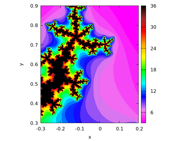 Categories: Package dynamics · Plotting ·
- Function: make_transform ([var1, var2, var3], fx, fy, fz) 
-
Returns a function suitable to be used in the option
transform_xyof plot3d. The three variables var1, var2, var3 are three dummy variable names, which represent the 3 variables given by the plot3d command (first the two independent variables and then the function that depends on those two variables). The three functions fx, fy, fz must depend only on those 3 variables, and will give the corresponding x, y and z coordinates that should be plotted. There are two transformations defined by default:polar_to_xyandspherical_to_xyz. See the documentation for those two transformations.Categories: Plotting ·
- Function: mandelbrot (options) 
-
Creates a graphic representation of the Mandelbrot set. This program is part of the additional package
dynamics, but that package does not have to be loaded; the first time mandelbrot is used, the package will be loaded automatically.This program can be called without any arguments, in which case it will use a default value of 9 iterations per point, a grid with dimensions set by the
gridplot option (default 30 by 30) and a region that extends from -2 to 2 in both axes. The options are all the same that plot2d accepts, plus an optioniterationsto change the number of iterations.Each pixel in the grid is given a color corresponding to the number of iterations it takes the sequence starting at zero to move out of the convergence circle of radius 2, centered at the origin. The maximum number of iterations is set by the option
iterations. The program uses its own default palette: magenta,violet, blue, cyan, green, yellow, orange, red, brown and black, but it can be changed by adding an explicitpaletteoption in the command. By default, the two axes are shown with the same scale, unless the optionyx_ratiois used or the optionsame_xyis disabled.Example:
[grid,400,400])$ incorrect syntax: end of file while scanning expression.
^
(%i1) mandelbrot ([iterations, 30], [x, -2, 1], [y, -1.2, 1.2],
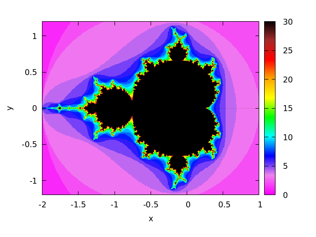 Categories: Package dynamics · Plotting ·
- System function: polar_to_xy 
-
It can be given as value for the
transform_xyoption of plot3d. Its effect will be to interpret the two independent variables in plot3d as the distance from the z axis and the azimuthal angle (polar coordinates), and transform them into x and y coordinates.Categories: Plotting ·
- Function: plot2d
plot2d (expr, range_x, options)
plot2d (expr_1=expr_2, range_x, range_y, options)
plot2d ([parametric, expr_x, expr_y, range], options)
plot2d ([discrete, points], options)
plot2d ([contour, expr], range_x, range_y, options)
plot2d ([type_1, …, type_n], options) ¶ -
There are 5 types of plots that can be plotted by
plot2d:- Explicit functions.
plot2d(expr, range_x, options), where expr is an expression that depends on only one variable, or the name of a function with one input parameter and numerical results. range_x is a list with three elements, the first one being the name of the variable that will be shown on the horizontal axis of the plot, and the other two elements should be two numbers, the first one smaller than the second, that define the minimum and maximum values to be shown on the horizontal axis. The name of the variable used in range_x must be the same variable on which expr depends. The result will show in the vertical axis the corresponding values of the expression or function for each value of the variable in the horizontal axis. - Implicit functions.
plot2d(expr_1=expr_2, range_x, range_y, options), where expr_1 and expr_2 are two expressions that can depend on one or two variables. range_x and range_y must be two lists of three elements that define the ranges for the variables in the two axes of the plot; the first element of each list is the name of the corresponding variable, and the other two elements are the minimum and maximum values for that variable. The two variables on which expr_1 and expr_2 can depend are those specified by range_x and range_y. The result will be a curve or a set of curves where the equation expr_1=expr_2 is true. - Parametric functions.
plot2d([parametric, expr_x, expr_y, range], options), where expr_x and expr_y are two expressions that depend on a single parameter. range must be a three-element list; the first element must be the name of the parameter on which expr_x and expr_y depend, and the other two elements must be the minimum and maximum values for that parameter. The result will be a curve in which the horizontal and vertical coordinates of each point are the values of expr_x and expr_y for a value of the parameter within the range given. - Set of points.
plot2d([discrete, points], options), displays a list of points, joined by segments by default. The horizontal and vertical coordinates of each of those points can be specified in three different ways: With two lists of the same length, in which the elements of the first list are the horizontal coordinates of the points and the second list are the vertical coordinates, or with a list of two-element lists, each one corresponding to the two coordinates of one of the points, or with a single list that defines the vertical coordinates of the points; in this last case, the horizontal coordinates of the n points will be assumed to be the first n natural numbers. - Contour lines.
plot2d([contour, expr], range_x, range_y, options), where expr is an expression that depends on two variables. range_x and range_y will be lists whose first elements are the names of those two variables, followed by two numbers that set the minimum and maximum values for them. The first variable will be represented along the horizontal axis and the second along the vertical axis. The result will be a set of curves along which the given expression has certain values. If those values are not specified with the optionlevels, plotd2d will try to choose, at the most, 8 values of the form d*10^n, where d is either 1, 2 or 5, all of them within the minimum and maximum values of expr within the given ranges.
At the end of a plot2d command several of the options described in
Plotting Optionscan be used. Many instances of the 5 types described above can be combined into a single plot, by putting them inside a list:plot2d([type_1, …, type_n], options). If one of the types included in the list require range_x or range_y, those ranges should come immediately after the list.If there are several plots to be plotted, a legend will be written to identity each of the expressions. The labels that should be used in that legend can be given with the option
legend. If that option is not used, Maxima will create labels from the expressions or function names.Examples:
- Explicit function.
(%i1) plot2d (sin(x), [x, -%pi, %pi])$
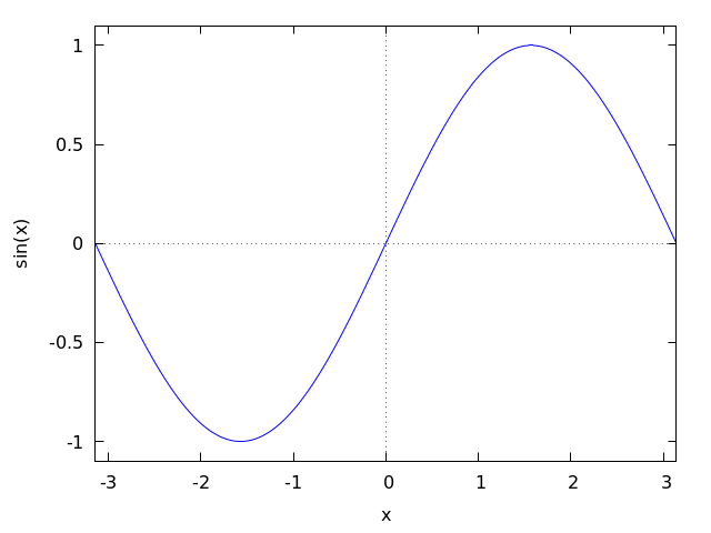
- Implicit function.
(%i1) plot2d (x^2-y^3+3*y=2, [x,-2.5,2.5], [y,-2.5,2.5])$
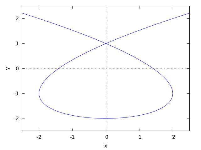
- Parametric function.
(%i1) r: (exp(cos(t))-2*cos(4*t)-sin(t/12)^5)$ (%i2) plot2d([parametric, r*sin(t), r*cos(t), [t,-8*%pi,8*%pi]])$
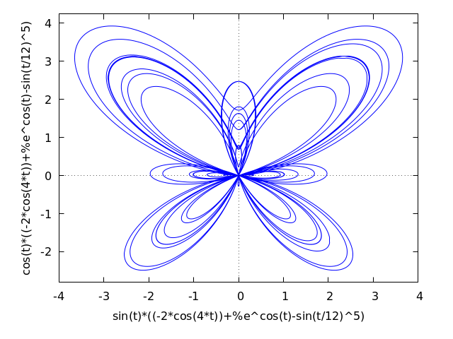
- Set of points.
(%i1) plot2d ([discrete, makelist(i*%pi, i, 1, 5), [0.6, 0.9, 0.2, 1.3, 1]])$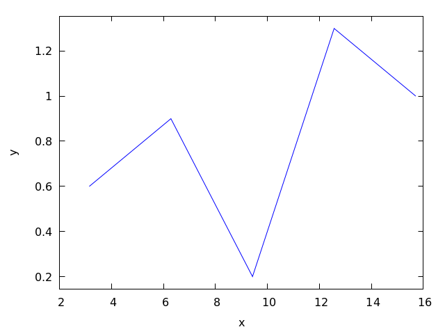
- Contour lines.
(%i1) plot2d ([contour, u^3 + v^2], [u, -4, 4], [v, -4, 4])$
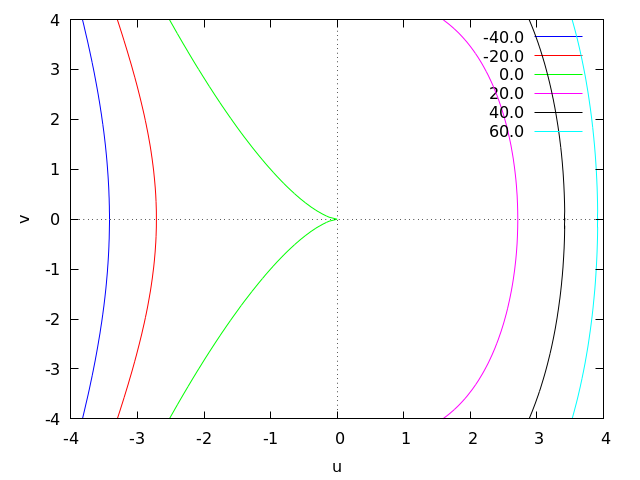
Examples using options.
If an explicit function grows too fast, the
yoption can be used to limit the values in the vertical axis:(%i1) plot2d (sec(x), [x, -2, 2], [y, -20, 20])$ plot2d: some values will be clipped.
When the plot box is disabled, no labels are created for the axes. In that case, instead of using
xlabelandylabelto set the names of the axes, it is better to use optionlabel, which allows more flexibility. Optionyx_ratiois used to change the default rectangular shape of the plot; in this example the plot will fill a square.(%i1) plot2d ( x^2 - 1, [x, -3, 3], nobox, grid2d, [yx_ratio, 1], [axes, solid], [xtics, -2, 4, 2], [ytics, 2, 2, 6], [label, ["x", 2.9, -0.3], ["x^2-1", 0.1, 8]], [title, "A parabola"])$
A plot with a logarithmic scale in the vertical axis:
(%i1) plot2d (exp(3*s), [s, -2, 2], logy)$
Plotting functions by name:
(%i1) F(x) := x^2 $
(%i2) :lisp (defun |$g| (x) (m* x x x)) $g
(%i2) H(x) := if x < 0 then x^4 - 1 else 1 - x^5 $ (%i3) plot2d ([F, G, H], [u, -1, 1], [y, -1.5, 1.5])$
Plot of a circumference of radius 1 centered at the origin, together with the function
y=-|x|. To prevent the circumference to look like an ellipse, optionsame_xyis used to scale the two axes at the same rate. Optionnolegendis also used to remove the legend identifying the two functions.(%i1) plot2d([x^2+y^2=1, -abs(x)], [x, -1.5, 1.5], [y, -2, 2], same_xy, nolegend); (%o1) false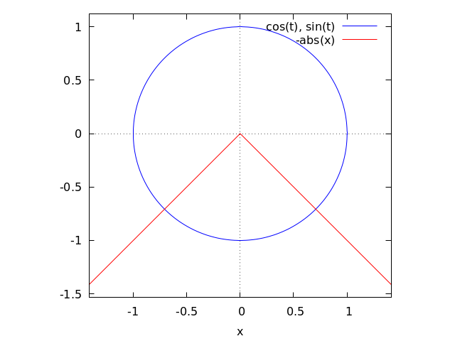
A plot of 200 random numbers between 0 and 9:
(%i1) plot2d ([discrete, makelist ( random(10), 200)])$
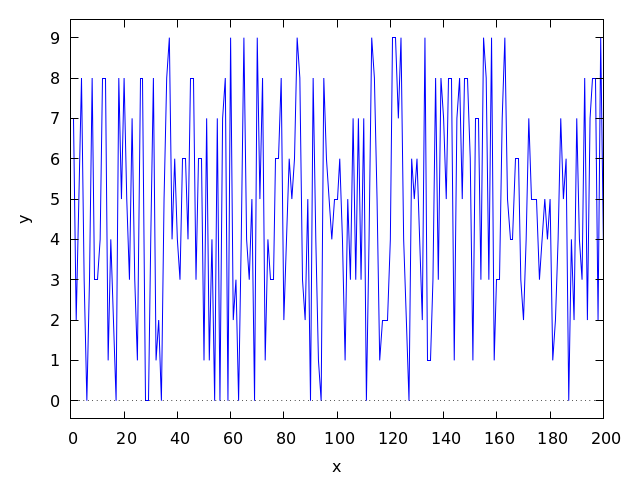
In the next example a table with three columns is saved in a file “data.txt” which is then read and the second and third column are plotted on the two axes:
(%i1) display2d:false$
(%i2) with_stdout ("data.txt", for x:0 thru 10 do print (x, x^2, x^3))$(%i3) data: read_matrix ("data.txt")$(%i4) plot2d ([discrete, transpose(data)[2], transpose(data)[3]], [style,points], [point_type,diamond], [color,red])$
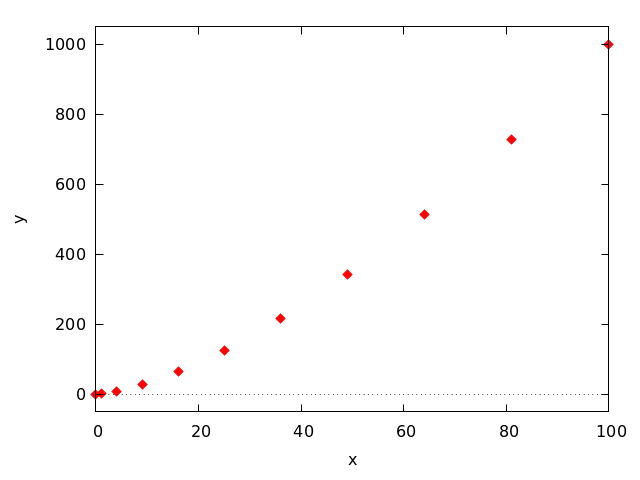
A plot of discrete data points together with a continuous function:
(%i1) xy: [[10, .6], [20, .9], [30, 1.1], [40, 1.3], [50, 1.4]]$
(%i2) plot2d([[discrete, xy], 2*%pi*sqrt(l/980)], [l,0,50], [style, points, lines], [color, red, blue], [point_type, asterisk], [legend, "experiment", "theory"], [xlabel, "pendulum's length (cm)"], [ylabel, "period (s)"])$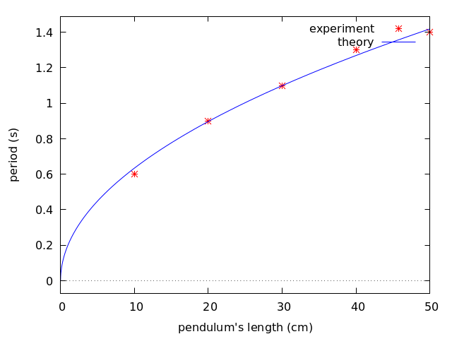
See also the
Plotting Optionssection.Categories: Plotting · - Explicit functions.
- Function: plot3d
plot3d (expr, x_range, y_range, …, options, …)
plot3d ([expr_1, …, expr_n], x_range, y_range, …, options, …) ¶ -
Displays a plot of one or more surfaces defined as functions of two variables or in parametric form.
The functions to be plotted may be specified as expressions or function names. The mouse can be used to rotate the plot looking at the surface from different sides.
Examples.
Plot of a function of two variables:
(%i1) plot3d (u^2 - v^2, [u, -2, 2], [v, -3, 3], [grid, 100, 100], nomesh_lines)$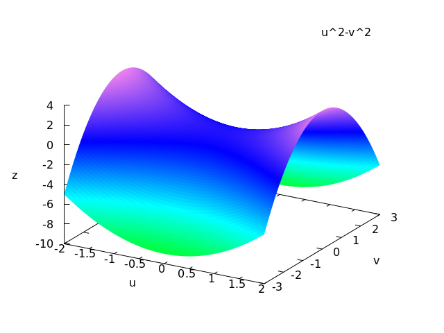
Use of the
zoption to limit a function that goes to infinity (in this case the function is minus infinity on the x and y axes); this also shows how to plot with only lines and no shading:(%i1) plot3d ( log ( x^2*y^2 ), [x, -2, 2], [y, -2, 2], [z, -8, 4], nopalette, [color, magenta])$ log: encountered log(0).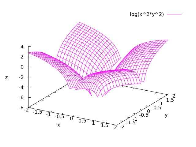
The infinite values of z can also be avoided by choosing a grid that does not fall on any points where the function is undefined, as in the next example, which also shows how to change the palette and how to include a color bar that relates colors to values of the z variable:
(%i1) plot3d (log (x^2*y^2), [x, -2, 2], [y, -2, 2],[grid, 29, 29], [palette, [gradient, red, orange, yellow, green]], color_bar, [xtics, 1], [ytics, 1], [ztics, 4], [color_bar_tics, 4])$ log: encountered log(0).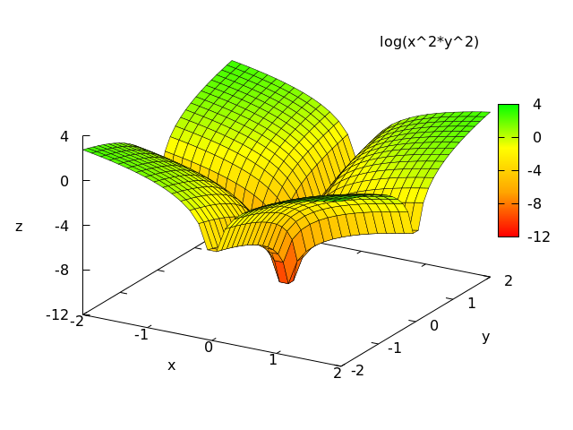
Two surfaces in the same plot. Ranges specific to one of the surfaces can be given by placing each expression and its ranges in a separate list; global ranges for the complete plot are also given after the function definitions.
(%i1) plot3d ([[-3*x - y, [x, -2, 2], [y, -2, 2]], 4*sin(3*(x^2 + y^2))/(x^2 + y^2), [x, -3, 3], [y, -3, 3]], [x, -4, 4], [y, -4, 4])$ expt: undefined: 0 to a negative exponent.
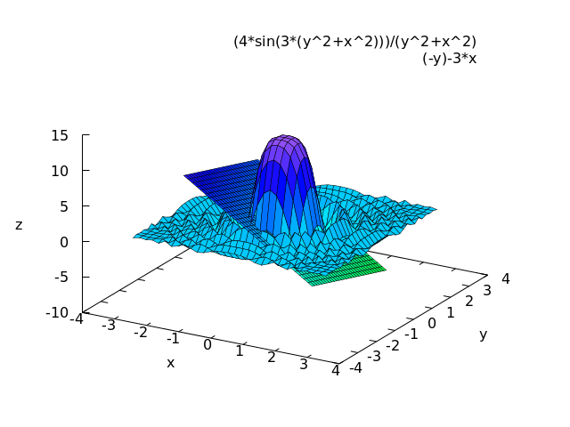
Plot of a Klein bottle, defined parametrically:
(%i1) expr_1: 5*cos(x)*(cos(x/2)*cos(y)+sin(x/2)*sin(2*y)+3)-10$ (%i2) expr_2: -5*sin(x)*(cos(x/2)*cos(y)+sin(x/2)*sin(2*y)+3)$ (%i3) expr_3: 5*(-sin(x/2)*cos(y)+cos(x/2)*sin(2*y))$
(%i4) plot3d ([expr_1, expr_2, expr_3], [x, -%pi, %pi], [y, -%pi, %pi], [grid, 50, 50])$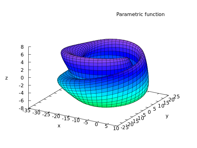
Plot of a “spherical harmonic” function, using the predefined transformation,
spherical_to_xyzto transform from spherical coordinates to rectangular coordinates. See the documentation forspherical_to_xyz.(%i1) plot3d (sin(2*theta)*cos(phi), [theta,0,%pi], [phi,0,2*%pi], [transform_xy, spherical_to_xyz], [grid, 30, 60], nolegend)$
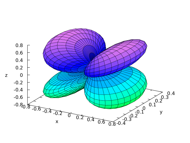
Use of the pre-defined function
polar_to_xyto transform from cylindrical to rectangular coordinates. See the documentation forpolar_to_xy.(%i1) plot3d (r^.33*cos(th/3), [r,0,1], [th,0,6*%pi], nobox, nolegend, [grid, 12, 80], [transform_xy, polar_to_xy])$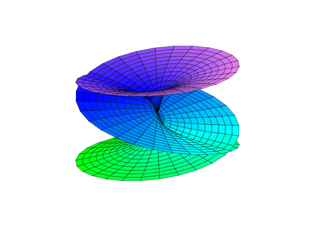
Plot of a sphere using the transformation from spherical to rectangular coordinates. Option
same_xyzis used to get the three axes scaled in the same proportion. When transformations are used, it is not convenient to eliminate the mesh lines, because Gnuplot will not show the surface correctly.(%i1) plot3d ( 5, [theta,0,%pi], [phi,0,2*%pi], same_xyz, nolegend, [transform_xy, spherical_to_xyz], [mesh_lines_color,blue], [palette,[gradient,"#1b1b4e", "#8c8cf8"]])$
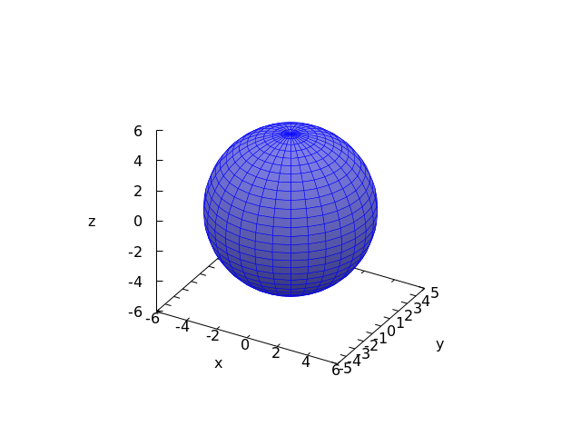
Definition of a function of two-variables using a matrix. Notice the single quote in the definition of the function, to prevent
plot3dfrom failing when it realizes that the matrix will require integer indices.(%i1) M: matrix([1,2,3,4], [1,2,3,2], [1,2,3,4], [1,2,3,3])$ (%i2) f(x, y) := float('M [round(x), round(y)])$ (%i3) plot3d (f(x,y), [x,1,4], [y,1,4], [grid,3,3], nolegend)$
By setting the elevation equal to zero, a surface can be seen as a map in which each color represents a different level.
(%i1) plot3d (cos (-x^2 + y^3/4), [x,-4,4], [y,-4,4], [zlabel,""], [mesh_lines_color,false], [elevation,0], [azimuth,0], color_bar, [grid,80,80], noztics, [color_bar_tics,1])$
See also
Plotting Options.Categories: Plotting ·
- System variable: plot_options 
-
This variable is being kept for compatibility with older versions of Wxmaxima, but its use is deprecated. To set global plotting options, see their current values or remove options, use
set_plot_option,get_plot_optionremove_plot_option, andreset_plot_options.Categories: Plotting ·
- Function: remove_plot_option (name) 
-
Removes the global value of an option. The name of the option must be given.
See also
set_plot_option,get_plot_optionandPlotting Options.Categories: Plotting ·
- Function: reset_plot_options () 
-
Sets the default global values of the plotting options. After changing the global values of some plotting options, this function is used to recovered the same values as when Maxima was started.
Categories: Plotting ·
- Function: set_plot_option (option) 
-
Accepts any of the options listed in the section
Plotting Options, and saves them for use in plotting commands. The values of the options set in each plotting command will have precedence, but if those options are not given, the default values set with this function will be used.set_plot_optionevaluates its argument and returns the complete list of options (after modifying the option given). If called without any arguments, it will simply show the list of current default options.See also
remove_plot_option,get_plot_optionand the section onPlotting Options.Example:
Modification of the
gridvalues.(%i1) set_plot_option ([grid, 30, 40]); (%o1) [[plot_format, gnuplot_pipes], [grid, 30, 40], [run_viewer, true], [axes, true], [nticks, 29], [adapt_depth, 5], [color, blue, red, green, magenta, black, cyan], [point_type, bullet, box, triangle, plus, times, asterisk], [palette, [hue, 0.33333333, 0.7, 1, 0.5], [hue, 0.8, 0.7, 1, 0.4]], [gnuplot_svg_background, white], [gnuplot_preamble, ], [gnuplot_term, default]]
Categories: Plotting ·
- System function: spherical_to_xyz 
-
It can be given as value for the
transform_xyoption ofplot3d. Its effect will be to interpret the two independent variables and the function inplot3das the spherical coordinates of a point (first, the angle with the z axis, then the angle of the xy projection with the x axis and finally the distance from the origin) and transform them into x, y and z coordinates.Categories: Plotting ·
- System variable: xmaxima_plot_command 
-
This variable stores the name of the command used to run the xmaxima program when the plot format is
xmaxima. Its default value is "xmaxima". If the xmaxima program is not found unless you give its complete path or if you want to try a different version of it, you may change the value of this variable. For instance,(%i1) xmaxima_plot_command: "/usr/local/bin/my_xmaxima"$
This variable must contain a string.
See also
gnuplot_commandandgeomview_command.Categories: Plotting ·
Next: Gnuplot Options, Previous: Functions and Variables for Plotting, Up: Plotting [Contents][Index]
14.4 Plotting Options
There is a variable plot_options which is kept for backward
compatibility with old versions of Wxmaxima but it is not used by the
plotting programs. The global options used by the plotting programs are
in a list which can only be accessed or modified in Maxima using
functions set_plot_option, get_plot_option,
remove_plot_option, and reset_plot_options.
Plotting options can also be included inside a plotting command, in which case they have effect only for that plotting command, without changing the global values of those options.
Plotting options consist of a list starting with one of the keywords in
this section, followed by one or more values. The options that accept
among their possible values true or false, can also be set to true by
simply writing their names, and false by writing their names with the
prefix no. For instance, typing logx as an option is equivalent
to writing [logx, true] and nobox is equivalent to
[box, false]. When just the name of the option is used for an
option which cannot have a value true, it means that any value
previously assigned to that option will be removed, leaving it to the
graphic program to decide what to do. There are also some abbreviations
for some options as will be shown below.
Some of the options may have different effects in different plotting commands as it will be pointed out for those particular options.
- Plot option: adapt_depth [adapt_depth, integer] 
Default value:
5The maximum number of splittings used by the adaptive plotting routine of
plot2d; integer must be a non-negative integer. A value of zero means that adaptive plotting will not be used and the resulting plot will have 1+4*nticks points (see optionnticks). To have more control on the number of points and their positions, a list of points can be created and then plotted using thediscretemethod ofplot2d.Categories: Plotting ·
- Plot option: axes [axes, symbol], axes, noaxes 
-
Default value:
trueWhere symbol can be either
true,false,x,yorsolid. Iffalse, no axes are shown; if equal toxoryonly the x or y axis will be shown; if it is equal totrue, both axes will be shown andsolidwill show the two axes with a solid line, rather than the default broken line. This option does not have any effect in the 3 dimensional plots. The single keywordsaxesandnoaxescan be used as synonyms for[axes, true]and[axes, false].Categories: Plotting ·
- Plot option: azimuth [azimuth, number] 
-
Default value:
30A plot3d plot can be thought of as starting with the x and y axis in the horizontal and vertical axis, as in plot2d, and the z axis coming out of the screen. The z axis is then rotated around the x axis through an angle equal to
elevationand then the new xy plane is rotated around the new z axis through an angleazimuth. This option sets the value for the azimuth, in degrees.See also
elevation.Categories: Plotting ·
- Plot option: box [box, symbol], box, nobox 
-
Default value:
trueIf set to
true, a bounding box will be drawn for the plot; if set tofalse, no box will be drawn. The single keywordsboxandnoboxcan be used as synonyms for[box, true]and[box, false].Categories: Plotting ·
- Plot option: color [color, color_1, …, color_n] 
-
In 2d plots it defines the color (or colors) for the various curves. In
plot3d, it defines the colors used for the mesh lines of the surfaces, when no palette is being used.If there are more curves or surfaces than colors, the colors will be repeated in sequence. The valid colors are
red,green,blue,magenta,cyan,yellow,orange,violet,brown,gray,black,white, or a string starting with the character # and followed by six hexadecimal digits: two for the red component, two for green component and two for the blue component. If the name of a given color is unknown color, black will be used instead.Categories: Plotting ·
- Plot option: color_bar [color_bar, symbol], color_bar, nocolor_bar 
-
Default value:
falsein plot3d,truein mandelbrot and juliaWhere symbol can be either
trueorfalse. Iftrue, wheneverplot3d,mandelbrotorjuliause a palette to represent different values, a box will be shown on the right, showing the corresponding between colors and values. The single keywordscolor_barandnocolor_barcan be used as synonyms for[color_bar, true]and[color_bar, false].Categories: Plotting ·
- Plot option: color_bar_tics [color_bar_tics, x1, x2, x3], color_bar_tics, nocolor_bar_tics 
-
Defines the values at which a mark and a number will be placed in the color bar. The first number is the initial value, the second the increments and the third is the last value where a mark is placed. The second and third numbers can be omitted. When only one number is given, it will be used as the increment from an initial value that will be chosen automatically. The single keyword
color_bar_ticsremoves a value given previously, making the graphic program use its default for the values of the tics andnocolor_bar_ticswill not show any tics on the color bar.Categories: Plotting ·
- Plot option: elevation [elevation, number] 
-
Default value:
60A plot3d plot can be thought of as starting with the x and y axis in the horizontal and vertical axis, as in plot2d, and the z axis coming out of the screen. The z axis is then rotated around the x axis through an angle equal to
elevationand then the new xy plane is rotated around the new z axis through an angleazimuth. This option sets the value for the elevation, in degrees.See also
azimuth.Categories: Plotting ·
- Plot option: gnuplot 
-
This is an abbreviation for
[plot_format, gnuplot]. Seeplot_format.Categories: Plotting ·
- Plot option: gnuplot_pipes 
-
This is an abbreviation for
[plot_format, gnuplot_pipes]. Seeplot_format.Categories: Plotting ·
- Plot option: grid [grid, integer, integer] 
Default value:
30,30Sets the number of grid points to use in the x- and y-directions for three-dimensional plotting or for the
juliaandmandelbrotprograms.For a way to actually draw a grid See
grid2d.Categories: Plotting ·
- Plot option: grid2d [grid2d, value], grid2d, nogrid2d 
-
Default value:
falseShows a grid of lines on the xy plane. The points where the grid lines are placed are the same points where tics are marked in the x and y axes, which can be controlled with the
xticsandyticsoptions. The single keywordsgrid2dandnogrid2dcan be used as synonyms for[grid2d, true]and[grid2d, false].See also
grid.Categories: Plotting ·
- Plot option: iterations [iterations, value] 
-
Default value:
9Number of iterations made by the programs mandelbrot and julia.
Categories: Plotting ·
- Plot option: label [label, [string, x, y], …] 
-
Writes one or several labels in the points with x, y coordinates indicated after each label.
Categories: Plotting ·
- Plot option: legend [legend, string_1, …, string_n], legend, nolegend 
-
It specifies the labels for the plots when various plots are shown. If there are more plots than the number of labels given, they will be repeated. If given the value
false, no legends will be shown. By default, the names of the expressions or functions will be used, or the words discrete1, discrete2, …, for discrete sets of points. The single keywordlegendremoves any previously defined legends, leaving it to the plotting program to set up a legend. The keywordnolegendis a synonym for[legend, false].Categories: Plotting ·
- Plot option: levels [levels, number, …] 
-
This option is used by
plot2dto do contour plots. If only one number is given after the keywordlevels, it must be a natural number;plot2dwill try to plot that number of contours with values between the minimum and maximum value of the expression given, with the form d*10^n, where d is either 1, 2 or 5. Since not always it will be possible to find that number of levels in that interval, the number of contour lines show will be smaller than the number specified by this option.If more than one number are given after the keyword
levels,plot2d. will show the contour lines corresponding to those values of the expression plotted, if they exist within the domain used.Categories: Plotting ·
- Plot option: logx [logx, value], logx, nologx 
-
Default value:
falseMakes the horizontal axes to be scaled logarithmically. It can be either true or false. The single keywords
logxandnologxcan be used as synonyms for[logx, true]and[logx, false].Categories: Plotting ·
- Plot option: logy [logy, value], logy, nology 
-
Default value:
falseMakes the vertical axes to be scaled logarithmically. It can be either true or false. The single keywords
logyandnologycan be used as synonyms for[logy, true]and[logy, false].Categories: Plotting ·
- Plot option: mesh_lines_color [mesh_lines_color, color], mesh_lines_color, nomesh_lines 
-
Default value:
blackIt sets the color used by plot3d to draw the mesh lines, when a palette is being used. It accepts the same colors as for the option
color(see the list of allowed colors incolor). It can also be given a valuefalseto eliminate completely the mesh lines. The single keywordmesh_lines_colorremoves any previously defined colors, leaving it to the graphic program to decide what color to use. The keywordnomesh_linesis a synonym for[mesh_lines_color, false]Categories: Plotting ·
- Plot option: nticks [nticks, integer] 
-
Default value:
29When plotting functions with
plot2d, it is gives the initial number of points used by the adaptive plotting routine for plotting functions. When plotting parametric functions withplot3d, it sets the number of points that will be shown for the plot.Categories: Plotting ·
- Plot option: palette [palette, [palette_1], …, [palette_n]], palette, nopalette 
-
It can consist of one palette or a list of several palettes. Each palette is a list with a keyword followed by values. If the keyword is gradient, it should be followed by a list of valid colors.
If the keyword is hue, saturation or value, it must be followed by 4 numbers. The first three numbers, which must be between 0 and 1, define the hue, saturation and value of a basic color to be assigned to the minimum value of z. The keyword specifies which of the three attributes (hue, saturation or value) will be increased according to the values of z. The last number indicates the increase corresponding to the maximum value of z. That last number can be bigger than 1 or negative; the corresponding values of the modified attribute will be rounded modulo 1.
Gnuplot only uses the first palette in the list; xmaxima will use the palettes in the list sequentially, when several surfaces are plotted together; if the number of palettes is exhausted, they will be repeated sequentially.
The color of the mesh lines will be given by the option
mesh_lines_color. Ifpaletteis given the valuefalse, the surfaces will not be shaded but represented with a mesh of curves only. In that case, the colors of the lines will be determined by the optioncolor.The single keyword
paletteremoves any palette previously defined, leaving it to the graphic program to decide the palette to use andnopaletteis a synonym for[palette, false].Categories: Plotting ·
- Plot option: plotepsilon [plotepsilon, value] 
-
Default value: 1e-6
This value is used by
plot2dwhen plotting implicit functions or contour lines. When plotting an explicit functionexpr_1=expr_2, it is converted intoexpr_1-expr_2and the points where that equals zero are searched. When a contour line forexprequal to some value is going to be plotted, the points whereexprminus that value are equal to zero are searched. The search is done by computing those expressions at a grid of points (seesample). If at one of the points in that grid the absolute value of the expression is less than the value ofplotepsilon, it will be assumed to be zero, and therefore, as being part of the curve to be plotted.Categories: Plotting ·
- Plot option: plot_format [plot_format, format], gnuplot, gnuplot_pipes, xmaxima 
-
Default value:
gnuplot, in Windows systems, orgnuplot_pipesin other systems.Where format is one of the following: gnuplot, xmaxima, mgnuplot, gnuplot_pipes or geomview. The three possibilities:
[plot_format, gnuplot],[plot_format, gnuplot_pipes]and[plot_format, xmaxima], can be abbreviated by the keywordsgnuplot,gnuplot_pipesandxmaxima.It sets the format to be used for plotting as explained in
Plotting Formats.Categories: Plotting ·
- Plot option: plot_realpart [plot_realpart, symbol], plot_realpart, noplot_realpart 
-
Default value:
falseIf set to
true, the functions to be plotted will be considered as complex functions whose real value should be plotted; this is equivalent to plottingrealpart(function). If set tofalse, nothing will be plotted when the function does not give a real value. For instance, whenxis negative,log(x)gives a complex value, with real value equal tolog(abs(x)); ifplot_realpartweretrue,log(-5)would be plotted aslog(5), while nothing would be plotted ifplot_realpartwerefalse. The single keywordplot_realpartcan be used as a synonym for[plot_realpart, true]andnoplot_realpartis a synonym for[plot_realpart, false].Categories: Plotting ·
- Plot option: point_type [point_type, type_1, …, type_n] 
-
In gnuplot, each set of points to be plotted with the style “points” or “linespoints” will be represented with objects taken from this list, in sequential order. If there are more sets of points than objects in this list, they will be repeated sequentially. The possible objects that can be used are:
bullet,circle,plus,times,asterisk,box,square,triangle,delta,wedge,nabla,diamond,lozenge.Categories: Plotting ·
- Plot option: pdf_file [pdf_file, file_name] 
-
Saves the plot into a PDF file with name equal to file_name, rather than showing it in the screen. By default, the file will be created in the directory defined by the variable
maxima_tempdir, unless file_name contains the character “/”, in which case it will be assumed to contain the complete path where the file should be created. The value ofmaxima_tempdircan be changed to save the file in a different directory. When the optiongnuplot_pdf_term_commandis also given, it will be used to set up Gnuplot’s PDF terminal; otherwise, Gnuplot’s pdfcairo terminal will be used with solid colored lines of width 3, plot size of 17.2 cm by 12.9 cm and font of 18 points.Categories: Plotting ·
- Plot option: png_file [png_file, file_name] 
-
Saves the plot into a PNG graphics file with name equal to file_name, rather than showing it in the screen. By default, the file will be created in the directory defined by the variable
maxima_tempdir, unless file_name contains the character “/”, in which case it will be assumed to contain the complete path where the file should be created. The value ofmaxima_tempdircan be changed to save the file in a different directory. When the optiongnuplot_png_term_commandis also given, it will be used to set up Gnuplot’s PNG terminal; otherwise, Gnuplot’s pngcairo terminal will be used, with a font of size 12.Categories: Plotting ·
- Plot option: ps_file [ps_file, file_name] 
-
Saves the plot into a Postscript file with name equal to file_name, rather than showing it in the screen. By default, the file will be created in the directory defined by the variable
maxima_tempdir, unless file_name contains the character “/”, in which case it will be assumed to contain the complete path where the file should be created. The value ofmaxima_tempdircan be changed to save the file in a different directory. When the optiongnuplot_ps_term_commandis also given, it will be used to set up Gnuplot’s Postscript terminal; otherwise, Gnuplot’s postscript terminal will be used with the EPS option, solid colored lines of width 2, plot size of 16.4 cm by 12.3 cm and font of 24 points.Categories: Plotting ·
- Plot option: run_viewer [run_viewer, symbol], run_viewer, norun_viewer 
-
Default value:
trueThis option is only used when the plot format is
gnuplotand the terminal isdefaultor when the Gnuplot terminal is set todumb(seegnuplot_term) and can have a true or false value.If the terminal is
default, a filerandom-string.gnuplot(or other name specified withgnuplot_out_file) is created with the gnuplot commands necessary to generate the plot. Optionrun_viewercontrols whether or not Gnuplot will be launched to execute those commands and show the plot.If the terminal is
default, gnuplot is run to execute the commands inrandom-string.gnuplot, producing another filemaxplot.txt(or other name specified withgnuplot_out_file). Optionrun_viewercontrols whether or not that file, with an ASCII representation of the plot, will be shown in the Maxima or Xmaxima console.Its default value, true, makes the plots appear in either the console or a separate graphics window.
run_viewerandnorun_viewerare synonyms for[run_viewer, true]and[run_viewer, false].Categories: Plotting ·
- Plot option: same_xy [same_xy , value], same_xy, nosame_xy 
-
It can be either true or false. If true, the scales used in the x and y axes will be the same, in either 2d or 3d plots. See also
yx_ratio.same_xyandnosame_xyare synonyms for[same_xy, true]and[same_xy, false].Categories: Plotting ·
- Plot option: same_xyz [same_xyz , value], same_xyz, nosame_xyz 
-
It can be either true or false. If true, the scales used in the 3 axes of a 3d plot will be the same.
same_xyzandnosame_xyzare synonyms for[same_xyz, true]and[same_xyz, false].Categories: Plotting ·
- Plot option: sample [sample, nx, ny] 
-
Default value:
[sample, 47, 47]nx and ny must be two natural numbers that will be used by
plot2dto look for the points that make part of the plot of an implicit function or a contour line. The domain is divided into nx intervals in the horizontal axis and ny intervals in the vertical axis and the numerical value of the expression is computed at the borders of those intervals. Higher values of nx and ny will give smoother curves, but will increase the time needed to trace the plot. When there are critical points in the plot where the curve changes direction, to get better results it is more important to try to make those points to be at the border of the intervals, rather than increasing nx and ny.Categories: Plotting ·
- Plot option: style [style, type_1, …, type_n], [style, [style_1], …, [style_n]] 
-
The styles that will be used for the various functions or sets of data in a 2d plot. The word style must be followed by one or more styles. If there are more functions and data sets than the styles given, the styles will be repeated. Each style can be either lines for line segments, points for isolated points, linespoints for segments and points, or dots for small isolated dots. Gnuplot accepts also an impulses style.
Each of the styles can be enclosed inside a list with some additional parameters. lines accepts one or two numbers: the width of the line and an integer that identifies a color. The default color codes are: 1: blue, 2: red, 3: magenta, 4: orange, 5: brown, 6: lime and 7: aqua. If you use Gnuplot with a terminal different than X11, those colors might be different; for example, if you use the option [gnuplot_term, ps], color index 4 will correspond to black, instead of orange.
points accepts one, two, or three parameters; the first parameter is the radius of the points, the second parameter is an integer that selects the color, using the same code used for lines and the third parameter is currently used only by Gnuplot and it corresponds to several objects instead of points. The default types of objects are: 1: filled circles, 2: open circles, 3: plus signs, 4: x, 5: *, 6: filled squares, 7: open squares, 8: filled triangles, 9: open triangles, 10: filled inverted triangles, 11: open inverted triangles, 12: filled lozenges and 13: open lozenges.
linespoints accepts up to five parameters: line width, points radius, color, type of object to replace the points, and the gnuplot pointinterval option to control space between points.
See also
colorandpoint_type.Categories: Plotting ·
- Plot option: svg_file [svg_file, file_name] 
-
Saves the plot into an SVG file with name equal to file_name, rather than showing it in the screen. By default, the file will be created in the directory defined by the variable
maxima_tempdir, unless file_name contains the character “/”, in which case it will be assumed to contain the complete path where the file should be created. The value ofmaxima_tempdircan be changed to save the file in a different directory. When the optiongnuplot_svg_term_commandis also given, it will be used to set up Gnuplot’s SVG terminal; otherwise, Gnuplot’s svg terminal will be used with font of 14 points.Categories: Plotting ·
- Plot option: title [title, text] 
-
Defines a title that will be written at the top of the plot.
Categories: Plotting ·
- Plot option: transform_xy [transform_xy, symbol], notransform_xy 
-
Where symbol is either
falseor the result obtained by using the functiontransform_xy. If different fromfalse, it will be used to transform the 3 coordinates in plot3d.notransform_xyremoves any transformation function previously defined.See
make_transform,polar_to_xyandspherical_to_xyz.Categories: Plotting ·
- Plot option: window [window, n] 
-
Opens the plot in window number n, instead of the default window 0. If window number n is already opened, the plot in that window will be replaced by the current plot.
Categories: Plotting ·
- Plot option: x [x, min, max] 
-
When used as the first option in a
plot2dcommand (or any of the first two inplot3d), it indicates that the first independent variable is x and it sets its range. It can also be used again after the first option (or after the second option in plot3d) to define the effective horizontal domain that will be shown in the plot.Categories: Plotting ·
- Plot option: xlabel [xlabel, string], noxlabel 
-
Specifies the string that will label the first axis; if this option is not used, that label will be the name of the independent variable, when plotting functions with
plot2dthe name of the first variable, when plotting surfaces withplot3d, or the first expression in the case of a parametric plot.noxlabelis equivalent to[xlabel, ""], which does not print any label on the first axis.Categories: Plotting ·
- Plot option: xmaxima 
-
This is an abbreviation for
[plot_format, xmaxima]. Seeplot_format.Categories: Plotting ·
- Plot option: xtics [xtics, x1, x2, x3], [xtics,
false], xtics, noxtics ¶ -
Defines the values at which a mark and a number will be placed in the x axis. The first number is the initial value, the second the increments and the third is the last value where a mark is placed. The second and third numbers can be omitted, in which case the first number is the increment from an initial value that will be chosen by the graphic program. If
[xtics, false]is used, no marks or numbers will be shown along the x axis.The single keyword
xticsremoves any values previously defined, leaving it to the graphic program to decide the values to use andnoxticsis a synonym for[xtics, false]Categories: Plotting ·
- Plot option: xy_scale [xy_scale, sx, sy] 
-
In a 2d plot, it defines the ratio of the total size of the Window to the size that will be used for the plot. The two numbers given as arguments are the scale factors for the x and y axes.
This option does not change the size of the graphic window or the placement of the graph in the window. If you want to change the aspect ratio of the plot, it is better to use option
yx_ratio. For instance,[yx_ratio, 10]instead of[xy_scale, 0.1, 1].Categories: Plotting ·
- Plot option: y [y, min, max] 
-
When used as one of the first two options in
plot3d, it indicates that one of the independent variables is y and it sets its range. Otherwise, it defines the effective domain of the second variable that will be shown in the plot.Categories: Plotting ·
- Plot option: ylabel [ylabel, string], noylabel 
-
Specifies the string that will label the second axis; if this option is not used, that label will be “y”, when plotting explicit functions with
plot2d, or the name of the second variable, when plotting surfaces withplot3d, or the second expression in the case of a parametric plot.noylabelis equivalent to[ylabel, ""], which does not print any label on the second axis.Categories: Plotting ·
- Plot option: ytics [ytics, y1, y2, y3], [ytics,
false], ytics, noytics ¶ -
Defines the values at which a mark and a number will be placed in the y axis. The first number is the initial value, the second the increments and the third is the last value where a mark is placed. The second and third numbers can be omitted, in which case the first number is the increment from an initial value that will be chosen by the graphic program. If
[ytics, false]is used, no marks or numbers will be shown along the y axis.The single keyword
yticsremoves any values previously defined, leaving it to the graphic program to decide the values to use andnoyticsis a synonym for[ytics, false]Categories: Plotting ·
- Plot option: yx_ratio [yx_ratio, r] 
-
In a 2d plot, the ratio between the vertical and the horizontal sides of the rectangle used to make the plot. See also
same_xy.Categories: Plotting ·
- Plot option: z [z, min, max] 
-
Used in
plot3dto set the effective range of values of z that will be shown in the plot.Categories: Plotting ·
- Plot option: zlabel [zlabel, string], nozlabel 
-
Specifies the string that will label the third axis, when using
plot3d. If this option is not used, that label will be “z”, when plotting surfaces, or the third expression in the case of a parametric plot. It can not be used withset_plot_optionand it will be ignored byplot2d.nozlabelis equivalent to[zlabel, ""], which does not print any label on the third axis.Categories: Plotting ·
- Plot option: zmin [zmin, z], zmin 
-
In 3d plots, the value of z that will be at the bottom of the plot box.
The single keyword
zminremoves any value previously defined, leaving it to the graphic program to decide the value to use.Categories: Plotting ·
- Plot option: ztics [ztics, z1, z2, z3], [ztics,
false], ztics, noztics ¶ -
Defines the values at which a mark and a number will be placed in the z axis. The first number is the initial value, the second the increments and the third is the last value where a mark is placed. The second and third numbers can be omitted, in which case the first number is the increment from an initial value that will be chosen by the graphic program. If
[ztics, false]is used, no marks or numbers will be shown along the z axis.The single keyword
zticsremoves any values previously defined, leaving it to the graphic program to decide the values to use andnozticsis a synonym for[ztics, false]Categories: Plotting ·
Next: Gnuplot_pipes Format Functions, Previous: Plotting Options, Up: Plotting [Contents][Index]
14.5 Gnuplot Options
There are several plot options specific to gnuplot. All of them consist of a keyword (the name of the option), followed by a string that should be a valid gnuplot command, to be passed directly to gnuplot. In most cases, there exist a corresponding plotting option that will produce a similar result and whose use is more recommended than the gnuplot specific option.
- Plot option: gnuplot_term [gnuplot_term, terminal_name] 
-
Sets the output terminal type for gnuplot. The argument terminal_name can be a string or one of the following 3 special symbols
- default (default value)
Gnuplot output is displayed in a separate graphical window and the gnuplot terminal used will be specified by the value of the option
gnuplot_default_term_command. - dumb
Gnuplot output is saved to a file
random-string.txtusing "ASCII art" approximation to graphics. If the optiongnuplot_out_fileis set to filename, the plot will be saved there, instead of the defaultrandom-string.gnuplot. The settings for the “dumb” terminal of Gnuplot are given by the value of optiongnuplot_dumb_term_command. If optionrun_vieweris set to true and the plot_format isgnuplotthat ASCII representation will also be shown in the Maxima or Xmaxima console. - ps
Gnuplot generates commands in the PostScript page description language. If the option
gnuplot_out_fileis set to filename, gnuplot writes the PostScript commands to filename. Otherwise, it is saved asmaxplot.psfile. The settings for this terminal are given by the value of the optiongnuplot_dumb_term_command. - A string representing any valid gnuplot term specification
Gnuplot can generate output in many other graphical formats such as png, jpeg, svg etc. To use those formats, option
gnuplot_termcan be set to any supported gnuplot term name (which must be a symbol) or even a full gnuplot term specification with any valid options (which must be a string). For example[gnuplot_term, png]creates output in PNG (Portable Network Graphics) format while[gnuplot_term, "png size 1000,1000"]creates PNG of 1000 x 1000 pixels size. If the optiongnuplot_out_fileis set to filename, gnuplot writes the output to filename. Otherwise, it is saved asmaxplot.termfile, where term is gnuplot terminal name.
Categories: Plotting · - default (default value)
- Plot option: gnuplot_out_file [gnuplot_out_file, file_name] 
-
It can be used to replace the default name for the file that contains the commands that will interpreted by gnuplot, when the terminal is set to
default, or to replace the default name of the graphic file that gnuplot creates, when the terminal is different fromdefault. If it contains one or more slashes, “/”, the name of the file will be left as it is; otherwise, it will be appended to the path of the temporary directory. The complete name of the files created by the plotting commands is always sent as output of those commands so they can be seen if the command is ended by semi-colon.Categories: Plotting ·
- Plot option: gnuplot_script_file [gnuplot_script_file, file_name_or_function] 
-
Creates a plot with
plot2d,plot3d,mandelbrotorjuliausing thegnuplotplot_formatand saving the script sent to Gnuplot in the file specified by file_name_or_function. The value file_name_or_function can be a string or a Maxima function of one variable that returns a string. If that string corresponds to a complete file path (directory and file name), the script will be created in that file and will not be deleted after Maxima is closed; otherwise, the string will give the name of a file to be created in the temporary directory and deleted when Maxima is closed.In this example, the script file name is set to “sin.gnuplot”, in the current directory.
(%i1) plot2d( sin(x), [x,0,2*%pi], [gnuplot_script_file, "./sin.gnuplot"]); (%o1) [./sin.gnuplot]
In this example,
gnuplot_prt(file)is a function that takes the default file name, file. It constructs a full file name for the data file by interpolating a random 8-digit integer with a pad of zeros into the default file name (a 16-character random string followed by “.gnuplot”). The temporary directory is determined bymaxima_tempdir(it is “/tmp” in this example).(%i1) gnuplot_prt(file) := block([beg,end], [beg,end] : split(file,"."), printf(false,"~a_~8,'0d.~a",beg,random(10^8-1),end)) $(%i2) plot2d( sin(x), [x,0,2*%pi], [gnuplot_script_file, gnuplot_prt]); (%o2) [/tmp/nxuo4x28s6wocvjw_99211646.gnuplot]
By default, the script would have been saved in a file named
random-string.gnuplot(random-string = nxuo4x28s6wocvjw_99211646 in this example) in the temporary directory. If the print statement in functiongnuplot_prtabove included a directory path, the file would have been saved in that directory rather than in the temporary directory.Categories: Plotting ·
- Plot option: gnuplot_pm3d [gnuplot_pm3d, value] 
-
With a value of
false, it can be used to disable the use of PM3D mode, which is enabled by default.Categories: Plotting ·
- Plot option: gnuplot_preamble [gnuplot_preamble, string] 
-
This option inserts gnuplot commands before any other commands sent to Gnuplot. Any valid gnuplot commands may be used. Multiple commands should be separated with a semi-colon. See also
gnuplot_postamble.Categories: Plotting ·
- Plot option: gnuplot_postamble [gnuplot_postamble, string] 
-
This option inserts gnuplot commands after other commands sent to Gnuplot and right before the plot command is sent. Any valid gnuplot commands may be used. Multiple commands should be separated with a semi-colon. See also
gnuplot_preamble.Categories: Plotting ·
- Plot option: gnuplot_default_term_command 
[gnuplot_default_term_command, command]
The gnuplot command to set the terminal type for the default terminal. It this option is not set, the command used will be:
"set term wxt size 640,480 font \",12\"; set term pop".Categories: Plotting ·
- Plot option: gnuplot_dumb_term_command 
[gnuplot_dumb_term_command, command]
The gnuplot command to set the terminal type for the dumb terminal. It this option is not set, the command used will be:
"set term dumb 79 22", which makes the text output 79 characters by 22 characters.Categories: Plotting ·
- Plot option: gnuplot_pdf_term_command [gnuplot_pdf_term_command, command] 
-
The gnuplot command to set the terminal type for the PDF terminal. If this option is not set, the command used will be:
"set term pdfcairo color solid lw 3 size 17.2 cm, 12.9 cm font \",18\"". See the gnuplot documentation for more information.Categories: Plotting ·
- Plot option: gnuplot_png_term_command [gnuplot_png_term_command, command] 
-
The gnuplot command to set the terminal type for the PNG terminal. If this option is not set, the command used will be:
"set term pngcairo font \",12\"". See the gnuplot documentation for more information.Categories: Plotting ·
- Plot option: gnuplot_ps_term_command [gnuplot_ps_term_command, command] 
-
The gnuplot command to set the terminal type for the PostScript terminal. If this option is not set, the command used will be:
"set term postscript eps color solid lw 2 size 16.4 cm, 12.3 cm font \",24\"". See the gnuplot documentation forset term postscriptfor more information.Categories: Plotting ·
- Plot option: gnuplot_strings [gnuplot_strings, value] 
-
With a value of
true, all strings used in labels and titles will be interpreted by gnuplot as “enhanced” text, if the terminal being used supports it. In enhanced mode, some characters such as ^ and _ are not printed, but interpreted as formatting characters. For a list of the formatting characters and their meaning, see the documentation for enhanced in Gnuplot. The default value for this option isfalse, which will not treat any characters as formatting characters.Categories: Plotting ·
- Plot option: gnuplot_svg_background
¶ -
[gnuplot_svg_background, color]
nognuplot_svg_backgroundSpecify the background color for SVG image output. color must be a string which specifies a color name recognized by Gnuplot, or an RGB triple of the form
"#xxxxxx"wherexis a hexadecimal digit. The default value is"white".When the value of
gnuplot_svg_backgroundisfalse, the background is the default determined by Gnuplot. At present (April 2023), the Gnuplot default is to specify the background in SVG output as"none".nognuplot_svg_background, specified by itself without a value, is equivalent to[gnuplot_svg_background, false].Categories: Plotting ·
- Plot option: gnuplot_svg_term_command [gnuplot_svg_term_command, command] 
-
The gnuplot command to set the terminal type for the SVG terminal. If this option is not set, the command used will be:
"set term svg font \",14\"". See the gnuplot documentation for more information.Categories: Plotting ·
- Plot option: gnuplot_curve_titles 
-
This is an obsolete option that has been replaced by
legenddescribed above.Categories: Plotting ·
- Plot option: gnuplot_curve_styles 
-
This is an obsolete option that has been replaced by
style.Categories: Plotting ·
Previous: Gnuplot Options, Up: Plotting [Contents][Index]
14.6 Gnuplot_pipes Format Functions
- Function: gnuplot_start () 
-
Opens the pipe to gnuplot used for plotting with the
gnuplot_pipesformat. Is not necessary to manually open the pipe before plotting.Categories: Plotting ·
- Function: gnuplot_close () 
-
Closes the pipe to gnuplot which is used with the
gnuplot_pipesformat.Categories: Plotting ·
- Function: gnuplot_send (s) 
-
Sends the command s to the gnuplot pipe. If that pipe is not currently opened, it will be opened before sending the command. s must be a string.
Categories: Plotting ·
- Function: gnuplot_restart () 
-
Closes the pipe to gnuplot which is used with the
gnuplot_pipesformat and opens a new pipe.Categories: Plotting ·
- Function: gnuplot_replot
gnuplot_replot ()
gnuplot_replot (s) ¶ -
Updates the gnuplot window. If
gnuplot_replotis called with a gnuplot command in a string s, thensis sent to gnuplot before reploting the window.Categories: Plotting ·
- Function: gnuplot_reset () 
-
Resets the state of gnuplot used with the
gnuplot_pipesformat. To update the gnuplot window callgnuplot_replotaftergnuplot_reset.Categories: Plotting ·
Next: Polynomials, Previous: Plotting [Contents][Index]
15 File Input and Output
- Comments
- Files
- Functions and Variables for File Input and Output
- Functions and Variables for TeX Output
- Functions and Variables for Fortran Output
Next: Files, Previous: File Input and Output, Up: File Input and Output [Contents][Index]
15.1 Comments
A comment in Maxima input is any text between /* and */.
The Maxima parser treats a comment as whitespace for the purpose of finding
tokens in the input stream; a token always ends at a comment. An input such as
a/* foo */b contains two tokens, a and b,
and not a single token ab. Comments are otherwise ignored by Maxima;
neither the content nor the location of comments is stored in parsed input
expressions.
Comments can be nested to arbitrary depth. The /* and */
delimiters form matching pairs. There must be the same number of /*
as there are */.
Examples:
(%i1) /* aa is a variable of interest */ aa : 1234; (%o1) 1234
(%i2) /* Value of bb depends on aa */ bb : aa^2; (%o2) 1522756
(%i3) /* User-defined infix operator */ infix ("b");
(%o3) b
(%i4) /* Parses same as a b c, not abc */ a/* foo */b/* bar */c; (%o4) a b c
(%i5) /* Comments /* can be nested /* to any depth */ */ */ 1 + xyz; (%o5) xyz + 1
Next: Functions and Variables for File Input and Output, Previous: Comments, Up: File Input and Output [Contents][Index]
15.2 Files
A file is simply an area on a particular storage device which contains data or text. Files on the disks are figuratively grouped into "directories". A directory is just a list of files. Commands which deal with files are:
appendfile batch batchload closefile file_output_append filename_merge file_search file_search_cache file_search_maxima file_search_lisp file_search_demo file_search_usage file_search_tests file_type file_type_lisp file_type_maxima load load_pathname loadfile loadprint pathname_directory pathname_name pathname_type printfile save stringout with_stdout writefile
When a file name is passed to functions like plot2d,
save, or writefile and the file name does not include a path,
Maxima stores the file in the current working directory. The current working
directory depends on the system like Windows or Linux and on the installation.
Next: Functions and Variables for TeX Output, Previous: Files, Up: File Input and Output [Contents][Index]
15.3 Functions and Variables for File Input and Output
- Function: appendfile (filename) 
-
Appends a console transcript to filename.
appendfileis the same aswritefile, except that the transcript file, if it exists, is always appended.closefilecloses the transcript file opened byappendfileorwritefile.Categories: File output · Console interaction ·
- Function: batch
batch (filename)
batch (filename, option)
batch (S)
batch (S, option) ¶ -
batch(filename)reads Maxima expressions from filename and evaluates them.batchsearches for filename in the listfile_search_maxima. See alsofile_search.batch(S)reads Maxima expressions from the input stream S as created byopenr. The behavior ofbatchin this case is the same as if the input were a file name, and in the remainder of this description, what is said about input files applies to input streams as well, except that the comments about searching for files do not apply to streams.batch(filename,is likedemo)demo(filename). In this casebatchsearches for filename in the listfile_search_demo. Seedemo.batch(filename,is liketest)run_testsuitewith the optiondisplay_all=true. For this casebatchsearches filename in the listfile_search_maximaand not in the listfile_search_testslikerun_testsuite. Furthermore,run_testsuiteruns tests which are in the listtestsuite_files. Withbatchit is possible to run any file in a test mode, which can be found in the listfile_search_maxima. This is useful, when writing a test file.filename comprises a sequence of Maxima expressions, each terminated with
;or$. The special variable%and the function%threfer to previous results within the file. The file may include:lispconstructs. Spaces, tabs, and newlines in the file are ignored. A suitable input file may be created by a text editor or by thestringoutfunction.batchreads each input expression from filename, displays the input to the console, computes the corresponding output expression, and displays the output expression. Input labels are assigned to the input expressions and output labels are assigned to the output expressions.batchevaluates every input expression in the file unless there is an error. If user input is requested (byasksignoraskinteger, for example)batchpauses to collect the requisite input and then continue; ifbatch_answers_from_fileistrue, the input is read from the file itself. See alsobatch_answers_from_file.It may be possible to halt
batchby typingcontrol-Cat the console. The effect ofcontrol-Cdepends on the underlying Lisp implementation.batchhas several uses, such as to provide a reservoir for working command lines, to give error-free demonstrations, or to help organize one’s thinking in solving complex problems.batchevaluates its arguments.When called with no second argument or with the option
demo,batchreturns the path of filename, if the argument is a file name, or the path of the file for which the input stream was opened, if the argument is a file input stream. If the argument is a string input stream, a representation of the input stream is returned.When called with the option
test, the return value is a an empty list[]or a list with filename and the numbers of the tests which have failed.See also
load,batchload,batch_answers_from_file, anddemo.Categories: Session management · File input ·
- Function: batchload
batchload (filename)
batchload (S) ¶ Reads Maxima expressions from input file filename or input stream S and evaluates them, without displaying the input or output expressions and without assigning labels to output expressions. Printed output (such as produced by
printordescribe)) is displayed, however.The special variable
%and the function%threfer to previous results from the interactive interpreter, not results within the file. The file cannot include:lispconstructs.batchloadevaluates its argument.batchloadreturns the path of filename, if the argument is a file name, or the path of the file for which the input stream was opened, if the argument is a file input stream. If the argument is a string input stream, a representation of the input stream is returned.Categories: Session management · File input ·
- Function: closefile () 
-
Closes the transcript file opened by
writefileorappendfile.Categories: File output · Console interaction ·
- Option variable: batch_answers_from_file 
Default value:
falseIf
true, thenbatchreads answers to interactive questions from its input file or stream.Example: Maxima’s interactive testsuite includes something like following.
[asksign (foo), sign (foo), sign (foo)]; p; [pos, pos, pos];
The first line makes Maxima ask a question; when
batch_answers_from_fileistrue, the second line is read as the answer to the question; and the third line provides the expected result.The command-line option
--batch-stringbindsbatch_answers_from_filetotrue. Therun_testsuitefunction, as a default, also bindsbatch_answers_from_filetotrue. See alsocommand_line_optionsandrun_testsuite.Categories: File input · Global flags ·
- Option variable: file_output_append 
Default value:
falsefile_output_appendgoverns whether file output functions append or truncate their output file. Whenfile_output_appendistrue, such functions append to their output file. Otherwise, the output file is truncated.save,stringout, andwith_stdoutrespectfile_output_append. Other functions which write output files do not respectfile_output_append. In particular, plotting and translation functions always truncate their output file, andtexandappendfilealways append.Categories: File output · Global flags ·
- Function: filename_merge (path, filename) 
-
Constructs a modified path from path and filename. If the final component of path is of the form
###.something, the component is replaced withfilename.something. Otherwise, the final component is simply replaced by filename.The result is a Lisp pathname object.
Categories: File input · File output ·
- Function: file_search
file_search (filename)
file_search (filename, pathlist) ¶ -
file_searchsearches for the file filename and returns the path to the file (as a string) if it can be found; otherwisefile_searchreturnsfalse.file_search (filename)searches in the default search directories, which are specified by thefile_search_maxima,file_search_lisp, andfile_search_demovariables.file_searchfirst checks if the actual name passed exists, before attempting to match it to “wildcard” file search patterns. Seefile_search_maximaconcerning file search patterns.The argument filename can be a path and file name, or just a file name, or, if a file search directory includes a file search pattern, just the base of the file name (without an extension). For example,
file_search ("/home/wfs/special/zeta.mac"); file_search ("zeta.mac"); file_search ("zeta");all find the same file, assuming the file exists and
/home/wfs/special/###.macis infile_search_maxima.file_search (filename, pathlist)searches only in the directories specified by pathlist, which is a list of strings. The argument pathlist supersedes the default search directories, so if the path list is given,file_searchsearches only the ones specified, and not any of the default search directories. Even if there is only one directory in pathlist, it must still be given as an one-element list.The user may modify the default search directories. See
file_search_maxima.file_searchis invoked byloadwithfile_search_maximaandfile_search_lispas the search directories.See also
file_search_cache.Categories: File input ·
- Option variable: file_search_cache 
Default value:
autofile_search_cachecontrols the use of a cache byfile_searchin order to speed up the search. Currently, it can only speed up searches where the filename part does not contain wildcards (but the directory part may).When
file_search_cacheisauto(the default value), the cache will be activated if a one-time check determines that the system (Lisp implementation, file system) fulfills the requirements. This can be overridden by settingfile_search_cachetotrue, which is not recommended. The valuefalseprevents the use of the cache.See also
file_search.Categories: File input ·
- Option variable: file_search_maxima 
- Option variable: file_search_lisp 
- Option variable: file_search_demo 
- Option variable: file_search_usage 
- Option variable: file_search_tests 
-
These variables specify lists of directories to be searched by
load,demo, and some other Maxima functions. The default values of these variables name various directories in the Maxima installation.The user can modify these variables, either to replace the default values or to append additional directories. For example,
file_search_maxima: ["/usr/local/foo/*.mac", "/usr/local/bar/*.mac"]$replaces the default value of
file_search_maxima, whilefile_search_maxima: append (file_search_maxima, ["/usr/local/foo/*.mac", "/usr/local/bar/*.mac"])$appends two additional directories. It may be convenient to put such an expression in the file
maxima-init.macso that the file search path is assigned automatically when Maxima starts. See also Introduction for Runtime Environment.Each element of the search list is a Common Lisp wildcard pathname. Briefly, a wildcard filename looks like
"*.lisp", which matches any filename with an extension of"lisp". A directory component of*matches any directory in the current directory, and**matches any directory and subdirectories in the current directory.So,
file_search_maximaincludes"/home/username/.maxima/**/*.mac". This means look in all subdirectories of"/home/username/.maxima/"for files with extension"mac". This includes subdirectories of subdirectories. Thus,load("file")will find"/home/username/.maxima/dir1/subdir1/file.mac".To only search for a single level of subdirectories, use
"/home/username/.maxima/*/*.mac". This means Maxima will not find the file"/home/username/.maxima/dir1/subdir1/file.mac"when Maxima tries to, say,load("file").Further information about Common Lisp pathnames maybe be found in CLHS Section 19.2: Pathnames.
Categories: File input · Global variables ·
- Function: file_type (filename) 
-
Returns a guess about the content of filename, based on the filename extension. filename need not refer to an actual file; no attempt is made to open the file and inspect the content.
The return value is a symbol, either
object,lisp, ormaxima. If the extension is matches one of the values infile_type_maxima,file_typereturnsmaxima. If the extension matches one of the values infile_type_lisp,file_typereturnslisp. If none of the above,file_typereturnsobject.See also
pathname_type.See
file_type_maximaandfile_type_lispfor the default values.Examples:
(%i1) map('file_type, ["test.lisp", "test.mac", "test.dem", "test.txt"]); (%o1) [lisp, maxima, maxima, object]Categories: File input ·
- Option variable: file_type_lisp 
Default value:
[l, lsp, lisp]file_type_lispis a list of file extensions that maxima recognizes as denoting a Lisp source file.See also
file_type.
- Option variable: file_type_maxima 
Default value:
[mac, mc, demo, dem, dm1, dm2, dm3, dmt, wxm]file_type_maximais a list of file extensions that maxima recognizes as denoting a Maxima source file.See also
file_type.
- Function: load (filename) 
-
Evaluates expressions in filename, thus bringing variables, functions, and other objects into Maxima. The binding of any existing object is clobbered by the binding recovered from filename.
filename must be a string, symbol, or Lisp pathname (as created by
filename_merge). To find the file,loadcallsfile_searchwithfile_search_maximaandfile_search_lispas the search directories. Ifloadsucceeds, it returns the name of the file. Otherwiseloadprints an error message.loadworks equally well for Lisp code and Maxima code. Files created bysave,translate_file, andcompile_file, which create Lisp code, andstringout, which creates Maxima code, can all be processed byload.loadcallsloadfileto load Lisp files andbatchloadto load Maxima files.loaddoes not recognize:lispconstructs in Maxima files, and while processing filename, the global variables_,__,%, and%thhave whatever bindings they had whenloadwas called.Note also that structures will only be read back as structures if they have been defined by
defstructbefore theloadcommand is called.See also
loadfile, for Lisp files; andbatch,batchload, anddemo. for Maxima files.See
file_searchfor more detail about the file search mechanism. Thenumericaliochapter describes many functions for loading csv and other data files.During Maxima file loading, the variable
load_pathnameis bound to the pathname of the file being loaded.loadevaluates its argument.Categories: Session management · File input ·
- System variable: load_pathname 
Default value:
falseWhen a file is loaded with the functions
load,loadfileorbatchloadthe system variableload_pathnameis bound to the pathname of the file which is processed.The variable
load_pathnamecan be accessed from the file during the loading.Example:
Suppose we have a batchfile
test.macin the directory"/home/dieter/workspace/mymaxima/temp/"with the following commandsprint("The value of load_pathname is: ", load_pathname)$ print("End of batchfile")$then we get the following output
(%i1) load("/home/dieter/workspace/mymaxima/temp/test.mac")$ The value of load_pathname is: /home/dieter/workspace/mymaxima/temp/test.mac End of batchfileCategories: File input ·
- Function: loadfile (filename) 
-
Evaluates Lisp expressions in filename.
loadfiledoes not invokefile_search, sofilenamemust include the file extension and as much of the path as needed to find the file.loadfilecan process files created bysave,translate_file, andcompile_file. The user may find it more convenient to useloadinstead ofloadfile.Categories: Session management · File input ·
- Option variable: loadprint 
Default value:
trueloadprinttells whether to print a message when a file is loaded.- When
loadprintistrue, always print a message. - When
loadprintis'loadfile, print a message only if a file is loaded by the functionloadfile. - When
loadprintis'autoload, print a message only if a file is automatically loaded. Seesetup_autoload. - When
loadprintisfalse, never print a message.
Categories: File input · Global flags ·- When
- Function: directory (path) 
-
Returns a list of the files and directories found in path in the file system.
path may contain wildcard characters (i.e., characters which represent unspecified parts of the path), which include at least the asterisk on most systems, and possibly other characters, depending on the system.
directoryrelies on the Lisp function DIRECTORY, which may have implementation-specific behavior.Categories: File input ·
- Function: pathname_directory (pathname) 
- Function: pathname_name (pathname) 
- Function: pathname_type (pathname) 
-
These functions return the components of pathname.
Examples:
(%i1) pathname_directory("/home/dieter/maxima/changelog.txt"); (%o1) /home/dieter/maxima/(%i2) pathname_name("/home/dieter/maxima/changelog.txt"); (%o2) changelog(%i3) pathname_type("/home/dieter/maxima/changelog.txt"); (%o3) txtCategories: File input ·
- Function: printfile (path) 
-
Prints the file named by path to the console. path may be a string or a symbol; if it is a symbol, it is converted to a string.
If path names a file which is accessible from the current working directory, that file is printed to the console. Otherwise,
printfileattempts to locate the file by appending path to each of the elements offile_search_usageviafilename_merge.printfilereturns path if it names an existing file, or otherwise the result of a successful filename merge.Categories: File input · Console interaction ·
- Function: save
save (filename, name_1, name_2, name_3, …)
save (filename, values, functions, labels, …)
save (filename, [m, n])
save (filename, name_1=expr_1, …)
save (filename, all)
save (filename, name_1=expr_1, name_2=expr_2, …) ¶ -
Stores the current values of name_1, name_2, name_3, …, in filename. The arguments are the names of variables, functions, or other objects. If a name has no value or function associated with it, it is ignored.
savereturns filename.savestores data in the form of Lisp expressions. If filename ends in.lispthe data stored bysavemay be recovered byload (filename). Seeload.The global flag
file_output_appendgoverns whethersaveappends or truncates the output file. Whenfile_output_appendistrue,saveappends to the output file. Otherwise,savetruncates the output file. In either case,savecreates the file if it does not yet exist.The special form
save (filename, values, functions, labels, ...)stores the items named byvalues,functions,labels, etc. The names may be any specified by the variableinfolists.valuescomprises all user-defined variables.The special form
save (filename, [m, n])stores the values of input and output labels m through n. Note that m and n must be literal integers. Input and output labels may also be stored one by one, e.g.,save ("foo.1", %i42, %o42).save (filename, labels)stores all input and output labels. When the stored labels are recovered, they clobber existing labels.The special form
save (filename, name_1=expr_1, name_2=expr_2, ...)stores the values of expr_1, expr_2, …, with names name_1, name_2, … It is useful to apply this form to input and output labels, e.g.,save ("foo.1", aa=%o88). The right-hand side of the equality in this form may be any expression, which is evaluated. This form does not introduce the new names into the current Maxima environment, but only stores them in filename.These special forms and the general form of
savemay be mixed at will. For example,save (filename, aa, bb, cc=42, functions, [11, 17]).The special form
save (filename, all)stores the current state of Maxima. This includes all user-defined variables, functions, arrays, etc., as well as some automatically defined items. The saved items include system variables, such asfile_search_maximaorshowtime, if they have been assigned new values by the user; seemyoptions.saveevaluates filename and quotes all other arguments.Categories: Session management · File output ·
- Function: stringout
stringout (filename, expr_1, expr_2, expr_3, …)
stringout (filename, [m, n])
stringout (filename, input)
stringout (filename, functions)
stringout (filename, values) ¶ -
stringoutwrites expressions to a file in the same form the expressions would be typed for input. The file can then be used as input for thebatchordemocommands, and it may be edited for any purpose.stringoutcan be executed whilewritefileis in progress.The global flag
file_output_appendgoverns whetherstringoutappends or truncates the output file. Whenfile_output_appendistrue,stringoutappends to the output file. Otherwise,stringouttruncates the output file. In either case,stringoutcreates the file if it does not yet exist.The general form of
stringoutwrites the values of one or more expressions to the output file. Note that if an expression is a variable, only the value of the variable is written and not the name of the variable. As a useful special case, the expressions may be input labels (%i1,%i2,%i3, …) or output labels (%o1,%o2,%o3, …).If
grindistrue,stringoutformats the output using thegrindformat. Otherwise thestringformat is used. Seegrindandstring.The special form
stringout (filename, [m, n])writes the values of input labels m through n, inclusive.The special form
stringout (filename, input)writes all input labels to the file.The special form
stringout (filename, functions)writes all user-defined functions (named by the global listfunctions)) to the file.The special form
stringout (filename, values)writes all user-assigned variables (named by the global listvalues)) to the file. Each variable is printed as an assignment statement, with the name of the variable, a colon, and its value. Note that the general form ofstringoutdoes not print variables as assignment statements.Categories: Session management · File output ·
- Function: with_stdout
with_stdout (f, expr_1, expr_2, expr_3, …)
with_stdout (s, expr_1, expr_2, expr_3, …) ¶ -
Evaluates expr_1, expr_2, expr_3, … and writes any output thus generated to a file f or output stream s. The evaluated expressions are not written to the output. Output may be generated by
print,display,grind, among other functions.The global flag
file_output_appendgoverns whetherwith_stdoutappends or truncates the output file f. Whenfile_output_appendistrue,with_stdoutappends to the output file. Otherwise,with_stdouttruncates the output file. In either case,with_stdoutcreates the file if it does not yet exist.with_stdoutreturns the value of its final argument.See also
writefileanddisplay2d.(%i1) with_stdout ("tmp.out", for i:5 thru 10 do print (i, "! yields", i!))$ (%i2) printfile ("tmp.out")$ 5 ! yields 120 6 ! yields 720 7 ! yields 5040 8 ! yields 40320 9 ! yields 362880 10 ! yields 3628800Categories: File output ·
- Function: writefile (filename) 
-
Begins writing a transcript of the Maxima session to filename. All interaction between the user and Maxima is then recorded in this file, just as it appears on the console.
As the transcript is printed in the console output format, it cannot be reloaded into Maxima. To make a file containing expressions which can be reloaded, see
saveandstringout.savestores expressions in Lisp form, whilestringoutstores expressions in Maxima form.The effect of executing
writefilewhen filename already exists depends on the underlying Lisp implementation; the transcript file may be clobbered, or the file may be appended.appendfilealways appends to the transcript file.It may be convenient to execute
playbackafterwritefileto save the display of previous interactions. Asplaybackdisplays only the input and output variables (%i1,%o1, etc.), any output generated by a print statement in a function (as opposed to a return value) is not displayed byplayback.closefilecloses the transcript file opened bywritefileorappendfile.Categories: File output · Console interaction ·
Next: Functions and Variables for Fortran Output, Previous: Functions and Variables for File Input and Output, Up: File Input and Output [Contents][Index]
15.4 Functions and Variables for TeX Output
Note that the built-in TeX output functionality of wxMaxima makes no use of the functions described here but uses its own implementation instead.
- Function: tex
tex (expr)
tex (expr, destination)
tex (expr, false)
tex (label)
tex (label, destination)
tex (label, false) ¶ -
Prints a representation of an expression suitable for the TeX document preparation system. The result is a fragment of a document, which can be copied into a larger document but not processed by itself.
tex (expr)prints a TeX representation of expr on the console.tex (label)prints a TeX representation of the expression named by label and assigns it an equation label (to be displayed to the left of the expression). The TeX equation label is the same as the Maxima label.destination may be an output stream or file name. When destination is a file name,
texappends its output to the file. The functionsopenwandopenacreate output streams.tex (expr, false)andtex (label, false)return their TeX output as a string.texevaluates its first argument after testing it to see if it is a label. Quote-quote''forces evaluation of the argument, thereby defeating the test and preventing the label.Examples:
(%i1) integrate (1/(1+x^3), x); 2 x - 1 2 atan(-------) log(x - x + 1) sqrt(3) log(x + 1) (%o1) - --------------- + ------------- + ---------- 6 sqrt(3) 3(%i2) tex (%o1); $$-\left({{\log \left(x^2-x+1\right)}\over{6}}\right)+{{\arctan \left({{2\,x-1}\over{\sqrt{3}}}\right)}\over{\sqrt{3}}}+{{\log \left(x+1\right)}\over{3}}\leqno{\tt (\%o1)}$$ (%o2) (\%o1)(%i3) tex (integrate (sin(x), x)); $$-\cos x$$ (%o3) false
(%i4) tex (%o1, "foo.tex"); (%o4) (\%o1)
tex (expr, false)returns its TeX output as a string.(%i1) S : tex (x * y * z, false); (%o1) $$x\,y\,z$$
(%i2) S; (%o2) $$x\,y\,z$$
Categories: TeX output · File output ·
- Function: tex1 (e) 
-
Returns a string which represents the TeX output for the expressions e. The TeX output is not enclosed in delimiters for an equation or any other environment.
Examples:
(%i1) tex1 (sin(x) + cos(x)); (%o1) \sin x+\cos x
- Function: texput
texput (a, s)
texput (a, f)
texput (a, s, operator_type)
texput (a, [s_1, s_2], matchfix)
texput (a, [s_1, s_2, s_3], matchfix) ¶ -
Assign the TeX output for the atom a, which can be a symbol or the name of an operator.
texput (a, s)causes thetexfunction to interpolate the string s into the TeX output in place of a.texput (a, f)causes thetexfunction to call the function f to generate TeX output. f must accept one argument, which is an expression which has operator a, and must return either a string (the TeX output) orfalse, indicating that the TeX function in effect whentexputis called should handle the expression. f may calltex1to generate TeX output for the arguments of the input expression.texput (a, s, operator_type), where operator_type isprefix,infix,postfix,nary, ornofix, causes thetexfunction to interpolate s into the TeX output in place of a, and to place the interpolated text in the appropriate position.texput (a, [s_1, s_2], matchfix)causes thetexfunction to interpolate s_1 and s_2 into the TeX output on either side of the arguments of a. The arguments (if more than one) are separated by commas.texput (a, [s_1, s_2, s_3], matchfix)causes thetexfunction to interpolate s_1 and s_2 into the TeX output on either side of the arguments of a, with s_3 separating the arguments.Examples:
Assign TeX output for a variable.
(%i1) texput (me,"\\mu_e"); (%o1) \mu_e
(%i2) tex (me); $$\mu_e$$ (%o2) false
Assign TeX output for an ordinary function (not an operator).
(%i1) texput (lcm, "\\mathrm{lcm}"); (%o1) \mathrm{lcm}(%i2) tex (lcm (a, b)); $$\mathrm{lcm}\left(a , b\right)$$ (%o2) falseCall a function to generate TeX output.
(%i1) texfoo (e) := block ([a, b], [a, b] : args (e), concat ("\\left[\\stackrel{",tex1(b),"}{",tex1(a),"}\\right]"))$(%i2) texput (foo, texfoo); (%o2) texfoo
(%i3) tex (foo (2^x, %pi)); $$\left[\stackrel{\pi}{2^{x}}\right]$$ (%o3) falseAssign TeX output for a prefix operator.
(%i1) prefix ("grad"); (%o1) grad(%i2) texput ("grad", " \\nabla ", prefix); (%o2) \nabla(%i3) tex (grad f); $$ \nabla f$$ (%o3) false
Assign TeX output for an infix operator.
(%i1) infix ("~"); (%o1) ~(%i2) texput ("~", " \\times ", infix); (%o2) \times(%i3) tex (a ~ b); $$a \times b$$ (%o3) false
Assign TeX output for a postfix operator.
(%i1) postfix ("##"); (%o1) ##(%i2) texput ("##", "!!", postfix); (%o2) !!(%i3) tex (x ##); $$x!!$$ (%o3) false
Assign TeX output for a nary operator.
(%i1) nary ("@@"); (%o1) @@(%i2) texput ("@@", " \\circ ", nary); (%o2) \circ(%i3) tex (a @@ b @@ c @@ d); $$a \circ b \circ c \circ d$$ (%o3) false
Assign TeX output for a nofix operator.
(%i1) nofix ("foo"); (%o1) foo(%i2) texput ("foo", "\\mathsc{foo}", nofix); (%o2) \mathsc{foo}(%i3) tex (foo); $$\mathsc{foo}$$ (%o3) falseAssign TeX output for a matchfix operator.
(%i1) matchfix ("<<", ">>"); (%o1) <<(%i2) texput ("<<", [" \\langle ", " \\rangle "], matchfix); (%o2) [ \langle , \rangle ](%i3) tex (<<a>>); $$ \langle a \rangle $$ (%o3) false
(%i4) tex (<<a, b>>); $$ \langle a , b \rangle $$ (%o4) false
(%i5) texput ("<<", [" \\langle ", " \\rangle ", " \\, | \\,"], matchfix); (%o5) [ \langle , \rangle , \, | \,](%i6) tex (<<a>>); $$ \langle a \rangle $$ (%o6) false
(%i7) tex (<<a, b>>); $$ \langle a \, | \,b \rangle $$ (%o7) false
Categories: TeX output ·
- Function: get_tex_environment (op) 
- Function: set_tex_environment (op, before, after) 
-
Customize the TeX environment output by
tex. As maintained by these functions, the TeX environment comprises two strings: one is printed before any other TeX output, and the other is printed after.Only the TeX environment of the top-level operator in an expression is output; TeX environments associated with other operators are ignored.
get_tex_environmentreturns the TeX environment which is applied to the operator op; returns the default if no other environment has been assigned.set_tex_environmentassigns the TeX environment for the operator op.Examples:
(%i1) get_tex_environment (":="); (%o1) [ \begin{verbatim} , ; \end{verbatim} ](%i2) tex (f (x) := 1 - x); \begin{verbatim} f(x):=1-x; \end{verbatim} (%o2) false(%i3) set_tex_environment (":=", "$$", "$$"); (%o3) [$$, $$](%i4) tex (f (x) := 1 - x); $$f(x):=1-x$$ (%o4) false
Categories: TeX output ·
- Function: get_tex_environment_default () 
- Function: set_tex_environment_default (before, after) 
-
Customize the TeX environment output by
tex. As maintained by these functions, the TeX environment comprises two strings: one is printed before any other TeX output, and the other is printed after.get_tex_environment_defaultreturns the TeX environment which is applied to expressions for which the top-level operator has no specific TeX environment (as assigned byset_tex_environment).set_tex_environment_defaultassigns the default TeX environment.Examples:
(%i1) get_tex_environment_default (); (%o1) [$$, $$]
(%i2) tex (f(x) + g(x)); $$g\left(x\right)+f\left(x\right)$$ (%o2) false
(%i3) set_tex_environment_default ("\\begin{equation} (%o3) [\begin{equation} , \end{equation}](%i4) ", " \begin{equation} g\left(x\right)+f\left(x\right) \end{equation} (%o4) false(%i5) \\end{equation}");Categories: TeX output ·
Previous: Functions and Variables for TeX Output, Up: File Input and Output [Contents][Index]
15.5 Functions and Variables for Fortran Output
- Option variable: fortindent 
Default value:
0fortindentcontrols the left margin indentation of expressions printed out by thefortrancommand.0gives normal printout (i.e., 6 spaces), and positive values will causes the expressions to be printed farther to the right.Categories: Translation and compilation ·
- Function: fortran (expr) 
-
Prints expr as a Fortran statement. The output line is indented with spaces. If the line is too long,
fortranprints continuation lines.fortranprints the exponentiation operator^as**, and prints a complex numbera + b %iin the form(a,b).expr may be an equation. If so,
fortranprints an assignment statement, assigning the right-hand side of the equation to the left-hand side. In particular, if the right-hand side of expr is the name of a matrix, thenfortranprints an assignment statement for each element of the matrix.If expr is not something recognized by
fortran, the expression is printed ingrindformat without complaint.fortrandoes not know about lists, arrays, or functions.fortindentcontrols the left margin of the printed lines.0is the normal margin (i.e., indented 6 spaces). Increasingfortindentcauses expressions to be printed further to the right.When
fortspacesistrue,fortranfills out each printed line with spaces to 80 columns.fortranevaluates its arguments; quoting an argument defeats evaluation.fortranalways returnsdone.See also the function
f90for printing one or more expressions as a Fortran 90 program.Examples:
(%i1) expr: (a + b)^12$
(%i2) fortran (expr); (b+a)**12 (%o2) done(%i3) fortran ('x=expr); x = (b+a)**12 (%o3) done(%i4) fortran ('x=expand (expr)); x = b**12+12*a*b**11+66*a**2*b**10+220*a**3*b**9+495*a**4*b**8+792 1 *a**5*b**7+924*a**6*b**6+792*a**7*b**5+495*a**8*b**4+220*a**9*b 2 **3+66*a**10*b**2+12*a**11*b+a**12 (%o4) done(%i5) fortran ('x=7+5*%i); x = (7,5) (%o5) done(%i6) fortran ('x=[1,2,3,4]); x(1) = 1 x(2) = 2 x(3) = 3 x(4) = 4 (%o6) done(%i7) f(x) := x^2$
(%i8) fortran (f); f (%o8) doneCategories: Translation and compilation ·
- Option variable: fortspaces 
Default value:
falseWhen
fortspacesistrue,fortranfills out each printed line with spaces to 80 columns.Categories: Translation and compilation ·
Next: Special Functions, Previous: File Input and Output [Contents][Index]
16 Polynomials
- Introduction to Polynomials
- Functions and Variables for Polynomials
- Introduction to algebraic extensions
- Functions and Variables for algebraic extensions
Next: Functions and Variables for Polynomials, Up: Polynomials [Contents][Index]
16.1 Introduction to Polynomials
Polynomials are stored in Maxima either in General Form or as Canonical
Rational Expressions (CRE) form. The latter is a standard form, and is
used internally by operations such as factor, ratsimp, and
so on.
Canonical Rational Expressions constitute a kind of representation
which is especially suitable for expanded polynomials and rational
functions (as well as for partially factored polynomials and rational
functions when ratfac is set to true). In this CRE form an
ordering of variables (from most to least main) is assumed for each
expression.
Polynomials are represented recursively by a list consisting of the main
variable followed by a series of pairs of expressions, one for each term
of the polynomial. The first member of each pair is the exponent of the
main variable in that term and the second member is the coefficient of
that term which could be a number or a polynomial in another variable
again represented in this form. Thus the principal part of the CRE form
of 3*x^2-1 is (X 2 3 0 -1) and that of 2*x*y+x-3
is (Y 1 (X 1 2) 0 (X 1 1 0 -3)) assuming y is the main
variable, and is (X 1 (Y 1 2 0 1) 0 -3) assuming x is the
main variable. "Main"-ness is usually determined by reverse alphabetical
order.
The "variables" of a CRE expression needn’t be atomic. In fact any
subexpression whose main operator is not +, -, *,
/ or ^ with integer power will be considered a "variable"
of the expression (in CRE form) in which it occurs. For example the CRE
variables of the expression x+sin(x+1)+2*sqrt(x)+1 are x,
sqrt(x), and sin(x+1). If the user does not specify an
ordering of variables by using the ratvars function Maxima will
choose an alphabetic one.
In general, CRE’s represent rational expressions, that is, ratios of
polynomials, where the numerator and denominator have no common factors,
and the denominator is positive. The internal form is essentially a pair
of polynomials (the numerator and denominator) preceded by the variable
ordering list. If an expression to be displayed is in CRE form or if it
contains any subexpressions in CRE form, the symbol /R/ will follow the
line label.
See the rat function for converting an expression to CRE form.
An extended CRE form is used for the representation of Taylor
series. The notion of a rational expression is extended so that the
exponents of the variables can be positive or negative rational numbers
rather than just positive integers and the coefficients can themselves
be rational expressions as described above rather than just polynomials.
These are represented internally by a recursive polynomial form which is
similar to and is a generalization of CRE form, but carries additional
information such as the degree of truncation. As with CRE form, the
symbol /T/ follows the line label of such expressions.
Next: Introduction to algebraic extensions, Previous: Introduction to Polynomials, Up: Polynomials [Contents][Index]
16.2 Functions and Variables for Polynomials
- Option variable: algebraic 
Default value:
falsealgebraicmust be set totruein order for the simplification of algebraic integers to take effect.Categories: Simplification flags and variables ·
- Option variable: berlefact 
Default value:
trueWhen
berlefactisfalsethen the Kronecker factoring algorithm will be used otherwise the Berlekamp algorithm, which is the default, will be used.Categories: Polynomials ·
- Function: bezout (p1, p2, x) 
-
an alternative to the
resultantcommand. It returns a matrix.determinantof this matrix is the desired resultant.Examples:
(%i1) bezout(a*x+b, c*x^2+d, x); [ b c - a d ] (%o1) [ ] [ a b ](%i2) determinant(%); 2 2 (%o2) a d + b c(%i3) resultant(a*x+b, c*x^2+d, x); 2 2 (%o3) a d + b cCategories: Polynomials ·
- Function: bothcoef (expr, x) 
-
Returns a list whose first member is the coefficient of x in expr (as found by
ratcoefif expr is in CRE form otherwise bycoeff) and whose second member is the remaining part of expr. That is,[A, B]whereexpr = A*x + B.Example:
(%i1) islinear (expr, x) := block ([c], c: bothcoef (rat (expr, x), x), is (freeof (x, c) and c[1] # 0))$(%i2) islinear ((r^2 - (x - r)^2)/x, x); (%o2) true
Categories: Polynomials ·
- Function: coeff
coeff (expr, x, n)
coeff (expr, x) ¶ -
Returns the coefficient of
x^nin expr, where expr is a polynomial or a monomial term in x. Other thanratcoefcoeffis a strictly syntactical operation and will only find literal instances ofx^nin the internal representation of expr.coeff(expr, x^n)is equivalent tocoeff(expr, x, n).coeff(expr, x, 0)returns the remainder of expr which is free of x. If omitted, n is assumed to be 1.x may be a simple variable or a subscripted variable, or a subexpression of expr which comprises an operator and all of its arguments.
It may be possible to compute coefficients of expressions which are equivalent to expr by applying
expandorfactor.coeffitself does not applyexpandorfactoror any other function.coeffdistributes over lists, matrices, and equations.See also
ratcoef.Examples:
coeffreturns the coefficientx^nin expr.(%i1) coeff (b^3*a^3 + b^2*a^2 + b*a + 1, a^3); 3 (%o1) bcoeff(expr, x^n)is equivalent tocoeff(expr, x, n).(%i1) coeff (c[4]*z^4 - c[3]*z^3 - c[2]*z^2 + c[1]*z, z, 3); (%o1) - c 3(%i2) coeff (c[4]*z^4 - c[3]*z^3 - c[2]*z^2 + c[1]*z, z^3); (%o2) - c 3coeff(expr, x, 0)returns the remainder of expr which is free of x.(%i1) coeff (a*u + b^2*u^2 + c^3*u^3, b, 0); 3 3 (%o1) c u + a ux may be a simple variable or a subscripted variable, or a subexpression of expr which comprises an operator and all of its arguments.
(%i1) coeff (h^4 - 2*%pi*h^2 + 1, h, 2); (%o1) - 2 %pi
(%i2) coeff (v[1]^4 - 2*%pi*v[1]^2 + 1, v[1], 2); (%o2) - 2 %pi
(%i3) coeff (sin(1+x)*sin(x) + sin(1+x)^3*sin(x)^3, sin(1+x)^3); 3 (%o3) sin (x)(%i4) coeff ((d - a)^2*(b + c)^3 + (a + b)^4*(c - d), a + b, 4); (%o4) c - d
coeffitself does not applyexpandorfactoror any other function.(%i1) coeff (c*(a + b)^3, a); (%o1) 0
(%i2) expand (c*(a + b)^3); 3 2 2 3 (%o2) b c + 3 a b c + 3 a b c + a c(%i3) coeff (%, a); 2 (%o3) 3 b c(%i4) coeff (b^3*c + 3*a*b^2*c + 3*a^2*b*c + a^3*c, (a + b)^3); (%o4) 0
(%i5) factor (b^3*c + 3*a*b^2*c + 3*a^2*b*c + a^3*c); 3 (%o5) (b + a) c(%i6) coeff (%, (a + b)^3); (%o6) c
coeffdistributes over lists, matrices, and equations.(%i1) coeff ([4*a, -3*a, 2*a], a); (%o1) [4, - 3, 2]
(%i2) coeff (matrix ([a*x, b*x], [-c*x, -d*x]), x); [ a b ] (%o2) [ ] [ - c - d ](%i3) coeff (a*u - b*v = 7*u + 3*v, u); (%o3) a = 7
Categories: Polynomials ·
- Function: content (p_1, x_1, …, x_n) 
-
Returns a list whose first element is the greatest common divisor of the coefficients of the terms of the polynomial p_1 in the variable x_n (this is the content) and whose second element is the polynomial p_1 divided by the content.
Examples:
(%i1) content (2*x*y + 4*x^2*y^2, y); 2 (%o1) [2 x, 2 x y + y]Categories: Polynomials ·
- Function: denom (expr) 
-
Returns the denominator of the rational expression expr.
See also
num(%i1) g1:(x+2)*(x+1)/((x+3)^2); (x + 1) (x + 2) (%o1) --------------- 2 (x + 3)(%i2) denom(g1); 2 (%o2) (x + 3)(%i3) g2:sin(x)/10*cos(x)/y; cos(x) sin(x) (%o3) ------------- 10 y(%i4) denom(g2); (%o4) 10 y
Categories: Expressions ·
- Function: divide (p_1, p_2, x_1, …, x_n) 
-
computes the quotient and remainder of the polynomial p_1 divided by the polynomial p_2, in a main polynomial variable, x_n. The other variables are as in the
ratvarsfunction. The result is a list whose first element is the quotient and whose second element is the remainder.Examples:
(%i1) divide (x + y, x - y, x); (%o1) [1, 2 y]
(%i2) divide (x + y, x - y); (%o2) [- 1, 2 x]
Note that
yis the main variable in the second example.Categories: Polynomials ·
- Function: eliminate ([eqn_1, …, eqn_n], [x_1, …, x_k]) 
-
Eliminates variables from equations (or expressions assumed equal to zero) by taking successive resultants. This returns a list of
n - kexpressions with the k variables x_1, …, x_k eliminated. First x_1 is eliminated yieldingn - 1expressions, thenx_2is eliminated, etc. Ifk = nthen a single expression in a list is returned free of the variables x_1, …, x_k. In this casesolveis called to solve the last resultant for the last variable.Example:
(%i1) expr1: 2*x^2 + y*x + z; 2 (%o1) z + x y + 2 x(%i2) expr2: 3*x + 5*y - z - 1; (%o2) - z + 5 y + 3 x - 1
(%i3) expr3: z^2 + x - y^2 + 5; 2 2 (%o3) z - y + x + 5(%i4) eliminate ([expr3, expr2, expr1], [y, z]); 8 7 6 5 4 (%o4) [7425 x - 1170 x + 1299 x + 12076 x + 22887 x 3 2 - 5154 x - 1291 x + 7688 x + 15376]Categories: Polynomials · Algebraic equations ·
- Function: ezgcd (p_1, p_2, p_3, …) 
-
Returns a list whose first element is the greatest common divisor of the polynomials p_1, p_2, p_3, … and whose remaining elements are the polynomials divided by the greatest common divisor. This always uses the
ezgcdalgorithm.See also
gcd,gcdex,gcdivide, andpoly_gcd.Examples:
The three polynomials have the greatest common divisor
2*x-3. The gcd is first calculated with the functiongcdand then with the functionezgcd.(%i1) p1 : 6*x^3-17*x^2+14*x-3; 3 2 (%o1) 6 x - 17 x + 14 x - 3(%i2) p2 : 4*x^4-14*x^3+12*x^2+2*x-3; 4 3 2 (%o2) 4 x - 14 x + 12 x + 2 x - 3(%i3) p3 : -8*x^3+14*x^2-x-3; 3 2 (%o3) - 8 x + 14 x - x - 3(%i4) gcd(p1, gcd(p2, p3)); (%o4) 2 x - 3
(%i5) ezgcd(p1, p2, p3); 2 3 2 2 (%o5) [2 x - 3, 3 x - 4 x + 1, 2 x - 4 x + 1, - 4 x + x + 1]Categories: Polynomials ·
- Option variable: facexpand 
Default value:
truefacexpandcontrols whether the irreducible factors returned byfactorare in expanded (the default) or recursive (normal CRE) form.Categories: Polynomials ·
- Function: factor
factor (expr)
factor (expr, p) ¶ -
Factors the expression expr, containing any number of variables or functions, into factors irreducible over the integers.
factor (expr, p)factors expr over the field of rationals with an element adjoined whose minimum polynomial is p.factorusesifactorsfunction for factoring integers.factorflagiffalsesuppresses the factoring of integer factors of rational expressions.dontfactormay be set to a list of variables with respect to which factoring is not to occur. (It is initially empty). Factoring also will not take place with respect to any variables which are less important (using the variable ordering assumed for CRE form) than those on thedontfactorlist.savefactorsiftruecauses the factors of an expression which is a product of factors to be saved by certain functions in order to speed up later factorizations of expressions containing some of the same factors.berlefactiffalsethen the Kronecker factoring algorithm will be used otherwise the Berlekamp algorithm, which is the default, will be used.intfaclimiftruemaxima will give up factorization of integers if no factor is found after trial divisions and Pollard’s rho method. If set tofalse(this is the case when the user callsfactorexplicitly), complete factorization of the integer will be attempted. The user’s setting ofintfaclimis used for internal calls tofactor. Thus,intfaclimmay be reset to prevent Maxima from taking an inordinately long time factoring large integers.factor_max_degreeif set to a positive integernwill prevent certain polynomials from being factored if their degree in any variable exceedsn.See also
collecttermsandsqfrExamples:
(%i1) factor (2^63 - 1); 2 (%o1) 7 73 127 337 92737 649657(%i2) factor (-8*y - 4*x + z^2*(2*y + x)); (%o2) (2 y + x) (z - 2) (z + 2)
(%i3) -1 - 2*x - x^2 + y^2 + 2*x*y^2 + x^2*y^2; 2 2 2 2 2 (%o3) x y + 2 x y + y - x - 2 x - 1(%i4) block ([dontfactor: [x]], factor (%/36/(1 + 2*y + y^2))); 2 (x + 2 x + 1) (y - 1) (%o4) ---------------------- 36 (y + 1)(%i5) factor (1 + %e^(3*x)); x 2 x x (%o5) (%e + 1) (%e - %e + 1)(%i6) factor (1 + x^4, a^2 - 2); 2 2 (%o6) (x - a x + 1) (x + a x + 1)(%i7) factor (-y^2*z^2 - x*z^2 + x^2*y^2 + x^3); 2 (%o7) - (y + x) (z - x) (z + x)(%i8) (2 + x)/(3 + x)/(b + x)/(c + x)^2; x + 2 (%o8) ------------------------ 2 (x + 3) (x + b) (x + c)(%i9) ratsimp (%); 4 3 (%o9) (x + 2)/(x + (2 c + b + 3) x 2 2 2 2 + (c + (2 b + 6) c + 3 b) x + ((b + 3) c + 6 b c) x + 3 b c )(%i10) partfrac (%, x); 2 4 3 (%o10) - (c - 4 c - b + 6)/((c + (- 2 b - 6) c 2 2 2 2 + (b + 12 b + 9) c + (- 6 b - 18 b) c + 9 b ) (x + c)) c - 2 - --------------------------------- 2 2 (c + (- b - 3) c + 3 b) (x + c) b - 2 + ------------------------------------------------- 2 2 3 2 ((b - 3) c + (6 b - 2 b ) c + b - 3 b ) (x + b) 1 - ---------------------------------------------- 2 ((b - 3) c + (18 - 6 b) c + 9 b - 27) (x + 3)(%i11) map ('factor, %); 2 c - 4 c - b + 6 c - 2 (%o11) - ------------------------- - ------------------------ 2 2 2 (c - 3) (c - b) (x + c) (c - 3) (c - b) (x + c) b - 2 1 + ------------------------ - ------------------------ 2 2 (b - 3) (c - b) (x + b) (b - 3) (c - 3) (x + 3)(%i12) ratsimp ((x^5 - 1)/(x - 1)); 4 3 2 (%o12) x + x + x + x + 1(%i13) subst (a, x, %); 4 3 2 (%o13) a + a + a + a + 1(%i14) factor (%th(2), %); 2 3 3 2 (%o14) (x - a) (x - a ) (x - a ) (x + a + a + a + 1)(%i15) factor (1 + x^12); 4 8 4 (%o15) (x + 1) (x - x + 1)(%i16) factor (1 + x^99); 2 6 3 (%o16) (x + 1) (x - x + 1) (x - x + 1) 10 9 8 7 6 5 4 3 2 (x - x + x - x + x - x + x - x + x - x + 1) 20 19 17 16 14 13 11 10 9 7 6 (x + x - x - x + x + x - x - x - x + x + x 4 3 60 57 51 48 42 39 33 - x - x + x + 1) (x + x - x - x + x + x - x 30 27 21 18 12 9 3 - x - x + x + x - x - x + x + 1)Categories: Polynomials ·
- Option variable: factor_max_degree 
Default value:
1000When
factor_max_degreeis set to a positive integern, it will prevent Maxima from attempting to factor certain polynomials whose degree in any variable exceedsn. Iffactor_max_degree_print_warningis true, a warning message will be printed.factor_max_degreecan be used to prevent excessive memory usage and/or computation time and stack overflows. Note that "obvious" factoring of polynomials such asx^2000+x^2001tox^2000*(x+1)will still take place. To disable this behavior, setfactor_max_degreeto0.Example:
(%i1) factor_max_degree : 100$
(%i2) factor(x^100-1); 2 4 3 2 (%o2) (x - 1) (x + 1) (x + 1) (x - x + x - x + 1) 4 3 2 8 6 4 2 (x + x + x + x + 1) (x - x + x - x + 1) 20 15 10 5 20 15 10 5 (x - x + x - x + 1) (x + x + x + x + 1) 40 30 20 10 (x - x + x - x + 1)(%i3) factor(x^101-1); 101 Refusing to factor polynomial x - 1 because its degree exceeds factor_max_degree (100) 101 (%o3) x - 1See also:
factor_max_degree_print_warningCategories: Polynomials ·
- Option variable: factor_max_degree_print_warning 
Default value:
trueWhen factor_max_degree_print_warning is true, then Maxima will print a warning message when the factoring of a polynomial is prevented because its degree exceeds the value of factor_max_degree.
See also:
factor_max_degreeCategories: Polynomials ·
- Option variable: factorflag 
Default value:
falseWhen
factorflagisfalse, suppresses the factoring of integer factors of rational expressions.Categories: Polynomials ·
- Function: factorout (expr, x_1, x_2, …) 
-
Rearranges the sum expr into a sum of terms of the form
f (x_1, x_2, …)*gwheregis a product of expressions not containing any x_i andfis factored.Note that the option variable
keepfloatis ignored byfactorout.Example:
(%i1) expand (a*(x+1)*(x-1)*(u+1)^2); 2 2 2 2 2 (%o1) a u x + 2 a u x + a x - a u - 2 a u - a(%i2) factorout(%,x); 2 (%o2) a u (x - 1) (x + 1) + 2 a u (x - 1) (x + 1) + a (x - 1) (x + 1)Categories: Expressions ·
- Function: factorsum (expr) 
-
Tries to group terms in factors of expr which are sums into groups of terms such that their sum is factorable.
factorsumcan recover the result ofexpand ((x + y)^2 + (z + w)^2)but it can’t recoverexpand ((x + 1)^2 + (x + y)^2)because the terms have variables in common.Example:
(%i1) expand ((x + 1)*((u + v)^2 + a*(w + z)^2)); 2 2 2 2 (%o1) a x z + a z + 2 a w x z + 2 a w z + a w x + v x 2 2 2 2 + 2 u v x + u x + a w + v + 2 u v + u(%i2) factorsum (%); 2 2 (%o2) (x + 1) (a (z + w) + (v + u) )Categories: Expressions ·
- Function: fasttimes (p_1, p_2) 
-
Returns the product of the polynomials p_1 and p_2 by using a special algorithm for multiplication of polynomials.
p_1andp_2should be multivariate, dense, and nearly the same size. Classical multiplication is of ordern_1 n_2wheren_1is the degree ofp_1andn_2is the degree ofp_2.fasttimesis of ordermax (n_1, n_2)^1.585.Categories: Polynomials ·
- Function: fullratsimp (expr) 
-
fullratsimprepeatedly appliesratsimpfollowed by non-rational simplification to an expression until no further change occurs, and returns the result.When non-rational expressions are involved, one call to
ratsimpfollowed as is usual by non-rational ("general") simplification may not be sufficient to return a simplified result. Sometimes, more than one such call may be necessary.fullratsimpmakes this process convenient.fullratsimp (expr, x_1, ..., x_n)takes one or more arguments similar toratsimpandrat.Example:
(%i1) expr: (x^(a/2) + 1)^2*(x^(a/2) - 1)^2/(x^a - 1); a/2 2 a/2 2 (x - 1) (x + 1) (%o1) ----------------------- a x - 1(%i2) ratsimp (expr); 2 a a x - 2 x + 1 (%o2) --------------- a x - 1(%i3) fullratsimp (expr); a (%o3) x - 1(%i4) rat (expr); a/2 4 a/2 2 (x ) - 2 (x ) + 1 (%o4)/R/ ----------------------- a x - 1Categories: Simplification functions · Rational expressions ·
- Function: fullratsubst (new, old, expr)
fullratsubst (old = new, expr)
fullratsubst ([ old_1 = new_1, …, old_n = new_n ], expr) ¶ -
fullratsubstapplieslratsubstrepeatedly until expr stops changing (orlrats_max_iteris reached). This function is useful when the replacement expression and the replaced expression have one or more variables in common.fullratsubstaccepts its arguments in the format ofratsubstorlratsubst.Examples:
-
substcan carry out multiple substitutions.lratsubstis analogous tosubst.
(%i1) subst ([a = b, c = d], a + c); (%o1) d + b
(%i2) lratsubst ([a^2 = b, c^2 = d], (a + e)*c*(a + c)); (%o2) (d + a c) e + a d + b c
- If only one substitution is desired, then a single equation may be given as first argument.
(%i1) lratsubst (a^2 = b, a^3); (%o1) a b
-
fullratsubstis equivalent toratsubstexcept that it recurses until its result stops changing.
(%i1) ratsubst (b*a, a^2, a^3); 2 (%o1) a b(%i2) fullratsubst (b*a, a^2, a^3); 2 (%o2) a b-
fullratsubstalso accepts a list of equations or a single equation as first argument.
(%i1) fullratsubst ([a^2 = b, b^2 = c, c^2 = a], a^3*b*c); (%o1) b
(%i2) fullratsubst (a^2 = b*a, a^3); 2 (%o2) a b-
fullratsubstcatches potential infinite recursions. lrats_max_iter.
Warning: fullratsubst2(listofeqns,expr): reached maximum iterations of 15 . Increase ‘lrats_max_iter’ to increase this limit.
(%i1) fullratsubst (b*a^2, a^2, a^3), lrats_max_iter=15; 3 15 (%o1) a bSee also
lrats_max_iterandfullratsubstflag.Categories: Rational expressions · -
- Option variable: fullratsubstflag 
Default value:
falseAn option variable that is set to
trueinfullratsubst.Categories: Polynomials · Rational expressions ·
- Function: gcd (p_1, p_2, x_1, …) 
-
Returns the greatest common divisor of p_1 and p_2. The flag
gcddetermines which algorithm is employed. Settinggcdtoez,subres,red, orspmodselects theezgcd, subresultantprs, reduced, or modular algorithm, respectively. Ifgcdfalsethengcd (p_1, p_2, x)always returns 1 for all x. Many functions (e.g.ratsimp,factor, etc.) cause gcd’s to be taken implicitly. For homogeneous polynomials it is recommended thatgcdequal tosubresbe used. To take the gcd when an algebraic is present, e.g.,gcd (x^2 - 2*sqrt(2)* x + 2, x - sqrt(2)), the option variablealgebraicmust betrueandgcdmust not beez.The
gcdflag, default:spmod, iffalsewill also prevent the greatest common divisor from being taken when expressions are converted to canonical rational expression (CRE) form. This will sometimes speed the calculation if gcds are not required.See also
ezgcd,gcdex,gcdivide, andpoly_gcd.Example:
(%i1) p1:6*x^3+19*x^2+19*x+6; 3 2 (%o1) 6 x + 19 x + 19 x + 6(%i2) p2:6*x^5+13*x^4+12*x^3+13*x^2+6*x; 5 4 3 2 (%o2) 6 x + 13 x + 12 x + 13 x + 6 x(%i3) gcd(p1, p2); 2 (%o3) 6 x + 13 x + 6(%i4) p1/gcd(p1, p2), ratsimp; (%o4) x + 1
(%i5) p2/gcd(p1, p2), ratsimp; 3 (%o5) x + xezgcdreturns a list whose first element is the greatest common divisor of the polynomials p_1 and p_2, and whose remaining elements are the polynomials divided by the greatest common divisor.(%i1) p1:6*x^3+19*x^2+19*x+6 $ (%i2) p2:6*x^5+13*x^4+12*x^3+13*x^2+6*x $
(%i3) ezgcd(p1, p2); 2 3 (%o3) [6 x + 13 x + 6, x + 1, x + x]Categories: Polynomials · Rational expressions ·
- Function: gcdex
gcdex (f, g)
gcdex (f, g, x) ¶ -
Returns a list
[a, b, u]where u is the greatest common divisor (gcd) of f and g, and u is equal toa f + b g. The arguments f and g should be univariate polynomials, or else polynomials in x a supplied main variable since we need to be in a principal ideal domain for this to work. The gcd means the gcd regarding f and g as univariate polynomials with coefficients being rational functions in the other variables.gcdeximplements the Euclidean algorithm, where we have a sequence ofL[i]: [a[i], b[i], r[i]]which are all perpendicular to[f, g, -1]and the next one is built as ifq = quotient(r[i]/r[i+1])thenL[i+2]: L[i] - q L[i+1], and it terminates atL[i+1]when the remainderr[i+2]is zero.The arguments f and g can be integers. For this case the function
igcdexis called bygcdex.See also
ezgcd,gcd,gcdivide, andpoly_gcd.Examples:
(%i1) gcdex (x^2 + 1, x^3 + 4); 2 x + 4 x - 1 x + 4 (%o1)/R/ [- ------------, -----, 1] 17 17(%i2) % . [x^2 + 1, x^3 + 4, -1]; (%o2)/R/ 0
Note that the gcd in the following is
1since we work ink(y)[x], not they+1we would expect ink[y, x].(%i1) gcdex (x*(y + 1), y^2 - 1, x); 1 (%o1)/R/ [0, ------, 1] 2 y - 1Categories: Polynomials · Rational expressions ·
- Function: gcfactor (n) 
-
Factors the Gaussian integer n over the Gaussian integers, i.e., numbers of the form
a + bwhere a and b are rational integers (i.e., ordinary integers). Factors are normalized by making a and b non-negative.%iCategories: Integers ·
- Function: gfactor (expr) 
-
Factors the polynomial expr over the Gaussian integers (that is, the integers with the imaginary unit
%iadjoined). This is likefactor (expr, a^2+1)where a is%i.Example:
(%i1) gfactor (x^4 - 1); (%o1) (x - 1) (x + 1) (x - %i) (x + %i)
Categories: Polynomials ·
- Function: gfactorsum (expr) 
-
is similar to
factorsumbut appliesgfactorinstead offactor.Categories: Expressions ·
- Function: hipow (expr, x) 
-
Returns the highest explicit exponent of x in expr. x may be a variable or a general expression. If x does not appear in expr,
hipowreturns0.hipowdoes not consider expressions equivalent toexpr. In particular,hipowdoes not expandexpr, sohipow (expr, x)andhipow (expand (expr, x))may yield different results.Examples:
(%i1) hipow (y^3 * x^2 + x * y^4, x); (%o1) 2
(%i2) hipow ((x + y)^5, x); (%o2) 1
(%i3) hipow (expand ((x + y)^5), x); (%o3) 5
(%i4) hipow ((x + y)^5, x + y); (%o4) 5
(%i5) hipow (expand ((x + y)^5), x + y); (%o5) 0
Categories: Expressions ·
- Option variable: intfaclim 
Default value: true
If
true, maxima will give up factorization of integers if no factor is found after trial divisions and Pollard’s rho method and factorization will not be complete.When
intfaclimisfalse(this is the case when the user callsfactorexplicitly), complete factorization will be attempted.intfaclimis set tofalsewhen factors are computed indivisors,divsumandtotient.Internal calls to
factorrespect the user-specified value ofintfaclim. Settingintfaclimtotruemay reduce the time spent factoring large integers.Categories: Integers ·
- Option variable: keepfloat 
Default value:
falseWhen
keepfloatistrue, prevents floating point numbers from being rationalized when expressions which contain them are converted to canonical rational expression (CRE) form.Note that the function
solveand those functions calling it (eigenvalues, for example) currently ignore this flag, converting floating point numbers anyway.Examples:
(%i1) rat(x/2.0); rat: replaced 0.5 by 1/2 = 0.5 x (%o1)/R/ - 2(%i2) rat(x/2.0), keepfloat; (%o2)/R/ 0.5 x
solveignoreskeepfloat:(%i1) solve(1.0-x,x), keepfloat; rat: replaced 1.0 by 1/1 = 1.0 (%o1) [x = 1]
Categories: Numerical evaluation ·
- Function: lopow (expr, x) 
-
Returns the lowest exponent of x which explicitly appears in expr. Thus
(%i1) lopow ((x+y)^2 + (x+y)^a, x+y); (%o1) min(2, a)
Categories: Expressions ·
- Function: lratsubst
lratsubst (new, old, expr)
lratsubst (old = new, expr)
lratsubst ([ old_1 = new_1, …, old_n = new_n ], expr) ¶ -
lratsubstis analogous tosubstexcept that it usesratsubstto perform substitutions.When
lratsubstis given two arguments, the first argument may be an equation, a list of equations, or a list of exactly one element, which is a list of equations.Substitutions are made in the order given by the list of equations, that is, from left to right.
Multiple substitutions are serial, not parallel. That is, later substitutions are performed on the results of earlier ones.
When
lratsubstis given three arguments new, old, and expr, it is equivalent tolratsubst(old = new, expr).Examples:
lratsubstcan carry out multiple substitutions.lratsubstis analogous tosubst.(%i1) lratsubst ([a = b, c = d], a + c); (%o1) d + b
(%i2) lratsubst ([a^2 = b, c^2 = d], (a + e)*c*(a + c)); (%o2) (d + a c) e + a d + b c
If only one substitution is desired, then a single equation may be given as first argument.
(%i1) lratsubst (a^2 = b, a^3); (%o1) a b
The first argument may be a list of exactly one element, which is a list of equations.
(%i1) lratsubst ([[a^2=b*a, b=c]], a^3); 2 (%o1) a cSee also
fullratsubst.Categories: Polynomials · Rational expressions ·
- Option variable: lrats_max_iter 
Default value:
100000The upper limit on the number of iterations that
fullratsubstandlratsubstmay perform. It must be set to a positive integer. See the example forfullratsubst.Categories: Polynomials · Rational expressions ·
- Option variable: modulus 
Default value:
falseWhen
modulusis a positive number p, operations on canonical rational expressions (CREs, as returned byratand related functions) are carried out modulo p, using the so-called "balanced" modulus system in whichn modulo pis defined as an integer k in[-(p-1)/2, ..., 0, ..., (p-1)/2]when p is odd, or[-(p/2 - 1), ..., 0, ...., p/2]when p is even, such thata p + kequals n for some integer a.If expr is already in canonical rational expression (CRE) form when
modulusis reset, then you may need to re-rat expr, e.g.,expr: rat (ratdisrep (expr)), in order to get correct results.Typically
modulusis set to a prime number. Ifmodulusis set to a positive non-prime integer, this setting is accepted, but a warning message is displayed. Maxima signals an error, when zero or a negative integer is assigned tomodulus.Examples:
(%i1) modulus:7; (%o1) 7
(%i2) polymod([0,1,2,3,4,5,6,7]); (%o2) [0, 1, 2, 3, - 3, - 2, - 1, 0]
(%i3) modulus:false; (%o3) false
(%i4) poly:x^6+x^2+1; 6 2 (%o4) x + x + 1(%i5) factor(poly); 6 2 (%o5) x + x + 1(%i6) modulus:13; (%o6) 13
(%i7) factor(poly); 2 4 2 (%o7) (x + 6) (x - 6 x - 2)(%i8) polymod(%); 6 2 (%o8) x + x + 1Categories: Integers ·
- Function: num (expr) 
-
Returns the numerator of expr if it is a ratio. If expr is not a ratio, expr is returned.
numevaluates its argument.See also
denom(%i1) g1:(x+2)*(x+1)/((x+3)^2); (x + 1) (x + 2) (%o1) --------------- 2 (x + 3)(%i2) num(g1); (%o2) (x + 1) (x + 2)
(%i3) g2:sin(x)/10*cos(x)/y; cos(x) sin(x) (%o3) ------------- 10 y(%i4) num(g2); (%o4) cos(x) sin(x)
Categories: Expressions ·
- Function: polydecomp (p, x) 
-
Decomposes the polynomial p in the variable x into the functional composition of polynomials in x.
polydecompreturns a list[p_1, ..., p_n]such thatlambda ([x], p_1) (lambda ([x], p_2) (... (lambda ([x], p_n) (x)) ...))
is equal to p. The degree of p_i is greater than 1 for i less than n.
Such a decomposition is not unique.
Examples:
(%i1) polydecomp (x^210, x); 7 5 3 2 (%o1) [x , x , x , x ](%i2) p : expand (subst (x^3 - x - 1, x, x^2 - a)); 6 4 3 2 (%o2) x - 2 x - 2 x + x + 2 x - a + 1(%i3) polydecomp (p, x); 2 3 (%o3) [x - a, x - x - 1]The following function composes
L = [e_1, ..., e_n]as functions inx; it is the inverse of polydecomp:(%i1) compose (L, x) := block ([r : x], for e in L do r : subst (e, x, r), r) $
Re-express above example using
compose:(%i1) compose (L, x) := block ([r : x], for e in L do r : subst (e, x, r), r) $
(%i2) polydecomp (compose ([x^2 - a, x^3 - x - 1], x), x); 2 3 (%o2) [x - a, x - x - 1]Note that though
compose (polydecomp (p, x), x)always returns p (unexpanded),polydecomp (compose ([p_1, ..., p_n], x), x)does not necessarily return[p_1, ..., p_n]:(%i1) compose (L, x) := block ([r : x], for e in L do r : subst (e, x, r), r) $
(%i2) polydecomp (compose ([x^2 + 2*x + 3, x^2], x), x); 2 2 (%o2) [x + 2, x + 1](%i3) polydecomp (compose ([x^2 + x + 1, x^2 + x + 1], x), x); 2 2 x + 3 x + 5 (%o3) [------, ------, 2 x + 1] 4 2Categories: Polynomials ·
- Function: polymod
polymod (p)
polymod (p, m) ¶ -
Converts the polynomial p to a modular representation with respect to the current modulus which is the value of the variable
modulus.polymod (p, m)specifies a modulus m to be used instead of the current value ofmodulus.See
modulus.Categories: Polynomials ·
- Function: polynomialp
polynomialp (p, L, coeffp, exponp)
polynomialp (p, L, coeffp)
polynomialp (p, L) ¶ -
Return
trueif p is a polynomial in the variables in the list L. The predicate coeffp must evaluate totruefor each coefficient, and the predicate exponp must evaluate totruefor all exponents of the variables in L. If you want to use a non-default value for exponp, you must supply coeffp with a value even if you want to use the default for coeffp.The command
polynomialp (p, L, coeffp)is equivalent topolynomialp (p, L, coeffp, 'nonnegintegerp)and the commandpolynomialp (p, L)is equivalent topolynomialp (p, L, 'constantp, 'nonnegintegerp).The polynomial needn’t be expanded:
(%i1) polynomialp ((x + 1)*(x + 2), [x]); (%o1) true
(%i2) polynomialp ((x + 1)*(x + 2)^a, [x]); (%o2) false
An example using non-default values for coeffp and exponp:
(%i1) polynomialp ((x + 1)*(x + 2)^(3/2), [x], numberp, numberp); (%o1) true
(%i2) polynomialp ((x^(1/2) + 1)*(x + 2)^(3/2), [x], numberp, numberp); (%o2) truePolynomials with two variables:
(%i1) polynomialp (x^2 + 5*x*y + y^2, [x]); (%o1) false
(%i2) polynomialp (x^2 + 5*x*y + y^2, [x, y]); (%o2) true
Polynomial in one variable and accepting any expression free of
xas a coefficient.(%i1) polynomialp (a*x^2 + b*x + c, [x]); (%o1) false
(%i2) polynomialp (a*x^2 + b*x + c, [x], lambda([ex], freeof(x, ex))); (%o2) true
Categories: Predicate functions · Polynomials ·
- Function: quotient
quotient (p_1, p_2)
quotient (p_1, p_2, x_1, …, x_n) ¶ -
Returns the polynomial p_1 divided by the polynomial p_2. The arguments x_1, …, x_n are interpreted as in
ratvars.quotientreturns the first element of the two-element list returned bydivide.Categories: Polynomials ·
- Function: rat
rat (expr)
rat (expr, x_1, …, x_n) ¶ -
Converts expr to canonical rational expression (CRE) form by expanding and combining all terms over a common denominator and cancelling out the greatest common divisor of the numerator and denominator, as well as converting floating point numbers to rational numbers within a tolerance of
ratepsilon. The variables are ordered according to the x_1, …, x_n, if specified, as inratvars.ratdoes not generally simplify functions other than addition+, subtraction-, multiplication*, division/, and exponentiation to an integer power, whereasratsimpdoes handle those cases. Note that atoms (numbers and variables) in CRE form are not the same as they are in the general form. For example,rat(x)- xyieldsrat(0)which has a different internal representation than 0.When
ratfacistrue,ratyields a partially factored form for CRE. During rational operations the expression is maintained as fully factored as possible without an actual call to the factor package. This should always save space and may save some time in some computations. The numerator and denominator are still made relatively prime (e.g.,rat((x^2 - 1)^4/(x + 1)^2)yields(x - 1)^4 (x + 1)^2whenratfacistrue), but the factors within each part may not be relatively prime.ratprintiffalsesuppresses the printout of the message informing the user of the conversion of floating point numbers to rational numbers.keepfloatiftrueprevents floating point numbers from being converted to rational numbers.See also
ratexpandandratsimp.Examples:
(%i1) ((x - 2*y)^4/(x^2 - 4*y^2)^2 + 1)*(y + a)*(2*y + x) / (4*y^2 + x^2); 4 (x - 2 y) (y + a) (2 y + x) (------------ + 1) 2 2 2 (x - 4 y ) (%o1) ------------------------------------ 2 2 4 y + x(%i2) rat (%, y, a, x); 2 a + 2 y (%o2)/R/ --------- x + 2 yCategories: Rational expressions ·
- Option variable: ratalgdenom 
Default value:
trueWhen
ratalgdenomistrue, allows rationalization of denominators with respect to radicals to take effect.ratalgdenomhas an effect only when canonical rational expressions (CRE) are used in algebraic mode.Categories: Simplification flags and variables ·
- Function: ratcoef
ratcoef (expr, x, n)
ratcoef (expr, x) ¶ -
Returns the coefficient of the expression
x^nin the expression expr. If omitted, n is assumed to be 1.The return value is free (except possibly in a non-rational sense) of the variables in x. If no coefficient of this type exists, 0 is returned.
ratcoefexpands and rationally simplifies its first argument and thus it may produce answers different from those ofcoeffwhich is purely syntactic. Thusratcoef ((x + 1)/y + x, x)returns(y + 1)/ywhereascoeffreturns 1.ratcoef (expr, x, 0), viewing expr as a sum, returns a sum of those terms which do not contain x. Therefore if x occurs to any negative powers,ratcoefshould not be used.Since expr is rationally simplified before it is examined, coefficients may not appear quite the way they were envisioned.
Example:
(%i1) s: a*x + b*x + 5$
(%i2) ratcoef (s, a + b); (%o2) x
Categories: Polynomials · Rational expressions ·
- Function: ratdenom (expr) 
-
Returns the denominator of expr, after coercing expr to a canonical rational expression (CRE). The return value is a CRE.
expr is coerced to a CRE by
ratif it is not already a CRE. This conversion may change the form of expr by putting all terms over a common denominator.denomis similar, but returns an ordinary expression instead of a CRE. Also,denomdoes not attempt to place all terms over a common denominator, and thus some expressions which are considered ratios byratdenomare not considered ratios bydenom.Categories: Rational expressions ·
- Option variable: ratdenomdivide 
Default value:
trueWhen
ratdenomdivideistrue,ratexpandexpands a ratio in which the numerator is a sum into a sum of ratios, all having a common denominator. Otherwise,ratexpandcollapses a sum of ratios into a single ratio, the numerator of which is the sum of the numerators of each ratio.Examples:
(%i1) expr: (x^2 + x + 1)/(y^2 + 7); 2 x + x + 1 (%o1) ---------- 2 y + 7(%i2) ratdenomdivide: true$
(%i3) ratexpand (expr); 2 x x 1 (%o3) ------ + ------ + ------ 2 2 2 y + 7 y + 7 y + 7(%i4) ratdenomdivide: false$
(%i5) ratexpand (expr); 2 x + x + 1 (%o5) ---------- 2 y + 7(%i6) expr2: a^2/(b^2 + 3) + b/(b^2 + 3); 2 b a (%o6) ------ + ------ 2 2 b + 3 b + 3(%i7) ratexpand (expr2); 2 b + a (%o7) ------ 2 b + 3Categories: Simplification flags and variables · Rational expressions ·
- Function: ratdiff (expr, x) 
-
Differentiates the rational expression expr with respect to x. expr must be a ratio of polynomials or a polynomial in x. The argument x may be a variable or a subexpression of expr.
The result is equivalent to
diff, although perhaps in a different form.ratdiffmay be faster thandiff, for rational expressions.ratdiffreturns a canonical rational expression (CRE) ifexpris a CRE. Otherwise,ratdiffreturns a general expression.ratdiffconsiders only the dependence of expr on x, and ignores any dependencies established bydepends.Example:
(%i1) expr: (4*x^3 + 10*x - 11)/(x^5 + 5); 3 4 x + 10 x - 11 (%o1) ---------------- 5 x + 5(%i2) ratdiff (expr, x); 7 5 4 2 8 x + 40 x - 55 x - 60 x - 50 (%o2) - --------------------------------- 10 5 x + 10 x + 25(%i3) expr: f(x)^3 - f(x)^2 + 7; 3 2 (%o3) f (x) - f (x) + 7(%i4) ratdiff (expr, f(x)); 2 (%o4) 3 f (x) - 2 f(x)(%i5) expr: (a + b)^3 + (a + b)^2; 3 2 (%o5) (b + a) + (b + a)(%i6) ratdiff (expr, a + b); 2 2 (%o6) 3 b + (6 a + 2) b + 3 a + 2 aCategories: Rational expressions ·
- Function: ratdisrep (expr) 
-
Returns its argument as a general expression. If expr is a general expression, it is returned unchanged.
Typically
ratdisrepis called to convert a canonical rational expression (CRE) into a general expression. This is sometimes convenient if one wishes to stop the "contagion", or use rational functions in non-rational contexts.See also
totaldisrep.Categories: Rational expressions ·
- Function: ratexpand (expr) 
- Option variable: ratexpand 
-
Expands expr by multiplying out products of sums and exponentiated sums, combining fractions over a common denominator, cancelling the greatest common divisor of the numerator and denominator, then splitting the numerator (if a sum) into its respective terms divided by the denominator.
The return value of
ratexpandis a general expression, even if expr is a canonical rational expression (CRE).The switch
ratexpandiftruewill cause CRE expressions to be fully expanded when they are converted back to general form or displayed, while if it isfalsethen they will be put into a recursive form. See alsoratsimp.When
ratdenomdivideistrue,ratexpandexpands a ratio in which the numerator is a sum into a sum of ratios, all having a common denominator. Otherwise,ratexpandcollapses a sum of ratios into a single ratio, the numerator of which is the sum of the numerators of each ratio.When
keepfloatistrue, prevents floating point numbers from being rationalized when expressions which contain them are converted to canonical rational expression (CRE) form.Examples:
(%i1) ratexpand ((2*x - 3*y)^3); 3 2 2 3 (%o1) - 27 y + 54 x y - 36 x y + 8 x(%i2) expr: (x - 1)/(x + 1)^2 + 1/(x - 1); x - 1 1 (%o2) -------- + ----- 2 x - 1 (x + 1)(%i3) expand (expr); x 1 1 (%o3) ------------ - ------------ + ----- 2 2 x - 1 x + 2 x + 1 x + 2 x + 1(%i4) ratexpand (expr); 2 2 x 2 (%o4) --------------- + --------------- 3 2 3 2 x + x - x - 1 x + x - x - 1Categories: Rational expressions ·
- Option variable: ratfac 
Default value:
falseWhen
ratfacistrue, canonical rational expressions (CRE) are manipulated in a partially factored form.During rational operations the expression is maintained as fully factored as possible without calling
factor. This should always save space and may save time in some computations. The numerator and denominator are made relatively prime, for examplefactor ((x^2 - 1)^4/(x + 1)^2)yields(x - 1)^4 (x + 1)^2, but the factors within each part may not be relatively prime.In the
ctensor(Component Tensor Manipulation) package, Ricci, Einstein, Riemann, and Weyl tensors and the scalar curvature are factored automatically whenratfacistrue.ratfacshould only be set for cases where the tensorial components are known to consist of few terms.The
ratfacandratweightschemes are incompatible and may not both be used at the same time.Categories: Rational expressions ·
- Function: ratnumer (expr) 
-
Returns the numerator of expr, after coercing expr to a canonical rational expression (CRE). The return value is a CRE.
expr is coerced to a CRE by
ratif it is not already a CRE. This conversion may change the form of expr by putting all terms over a common denominator.numis similar, but returns an ordinary expression instead of a CRE. Also,numdoes not attempt to place all terms over a common denominator, and thus some expressions which are considered ratios byratnumerare not considered ratios bynum.Categories: Rational expressions ·
- Function: ratp (expr) 
-
Returns
trueif expr is a canonical rational expression (CRE) or extended CRE, otherwisefalse.CRE are created by
ratand related functions. Extended CRE are created bytaylorand related functions.Categories: Predicate functions · Rational expressions ·
- Option variable: ratprint 
Default value:
trueWhen
ratprintistrue, a message informing the user of the conversion of floating point numbers to rational numbers is displayed.
- Function: ratsimp (expr) 
- Function: ratsimp (expr, x_1, …, x_n) 
-
Simplifies the expression expr and all of its subexpressions, including the arguments to non-rational functions. The result is returned as the quotient of two polynomials in a recursive form, that is, the coefficients of the main variable are polynomials in the other variables. Variables may include non-rational functions (e.g.,
sin (x^2 + 1)) and the arguments to any such functions are also rationally simplified.ratsimp (expr, x_1, ..., x_n)enables rational simplification with the specification of variable ordering as inratvars.When
ratsimpexponsistrue,ratsimpis applied to the exponents of expressions during simplification.See also
ratexpand. Note thatratsimpis affected by some of the flags which affectratexpand.Examples:
(%i1) sin (x/(x^2 + x)) = exp ((log(x) + 1)^2 - log(x)^2); 2 2 x (log(x) + 1) - log (x) (%o1) sin(------) = %e 2 x + x(%i2) ratsimp (%); 1 2 (%o2) sin(-----) = %e x x + 1(%i3) ((x - 1)^(3/2) - (x + 1)*sqrt(x - 1))/sqrt((x - 1)*(x + 1)); 3/2 (x - 1) - sqrt(x - 1) (x + 1) (%o3) -------------------------------- sqrt((x - 1) (x + 1))(%i4) ratsimp (%); 2 sqrt(x - 1) (%o4) - ------------- 2 sqrt(x - 1)(%i5) x^(a + 1/a), ratsimpexpons: true; 2 a + 1 ------ a (%o5) xCategories: Simplification functions · Rational expressions ·
- Option variable: ratsimpexpons 
Default value:
falseWhen
ratsimpexponsistrue,ratsimpis applied to the exponents of expressions during simplification.Categories: Simplification flags and variables · Rational expressions ·
- Option variable: radsubstflag 
Default value:
falseradsubstflag, iftrue, permitsratsubstto make substitutions such asuforsqrt (x)inx.Categories: Simplification flags and variables ·
- Function: ratsubst (a, b, c) 
-
Substitutes a for b in c and returns the resulting expression. b may be a sum, product, power, etc.
ratsubstknows something of the meaning of expressions whereassubstdoes a purely syntactic substitution. Thussubst (a, x + y, x + y + z)returnsx + y + zwhereasratsubstreturnsz + a.When
radsubstflagistrue,ratsubstmakes substitutions for radicals in expressions which don’t explicitly contain them.ratsubstignores the valuetrueof the option variableskeepfloat,float, andnumer.Examples:
(%i1) ratsubst (a, x*y^2, x^4*y^3 + x^4*y^8); 3 4 (%o1) a x y + a(%i2) cos(x)^4 + cos(x)^3 + cos(x)^2 + cos(x) + 1; 4 3 2 (%o2) cos (x) + cos (x) + cos (x) + cos(x) + 1(%i3) ratsubst (1 - sin(x)^2, cos(x)^2, %); 4 2 2 (%o3) sin (x) - 3 sin (x) + cos(x) (2 - sin (x)) + 3(%i4) ratsubst (1 - cos(x)^2, sin(x)^2, sin(x)^4); 4 2 (%o4) cos (x) - 2 cos (x) + 1(%i5) radsubstflag: false$
(%i6) ratsubst (u, sqrt(x), x); (%o6) x
(%i7) radsubstflag: true$
(%i8) ratsubst (u, sqrt(x), x); 2 (%o8) uCategories: Rational expressions ·
- Function: ratvars (x_1, …, x_n) 
- Function: ratvars () 
- System variable: ratvars 
-
Declares main variables x_1, …, x_n for rational expressions. x_n, if present in a rational expression, is considered the main variable. Otherwise, x_[n-1] is considered the main variable if present, and so on through the preceding variables to x_1, which is considered the main variable only if none of the succeeding variables are present.
If a variable in a rational expression is not present in the
ratvarslist, it is given a lower priority than x_1.The arguments to
ratvarscan be either variables or non-rational functions such assin(x).The variable
ratvarsis a list of the arguments of the functionratvarswhen it was called most recently. Each call to the functionratvarsresets the list.ratvars ()clears the list.Categories: Rational expressions ·
- Option variable: ratvarswitch 
Default value:
trueMaxima keeps an internal list in the Lisp variable
VARLISTof the main variables for rational expressions. Ifratvarswitchistrue, every evaluation starts with a fresh listVARLIST. This is the default behavior. Otherwise, the main variables from previous evaluations are not removed from the internal listVARLIST.The main variables, which are declared with the function
ratvarsare not affected by the option variableratvarswitch.Examples:
If
ratvarswitchistrue, every evaluation starts with a fresh listVARLIST.(%i1) ratvarswitch:true$
(%i2) rat(2*x+y^2); 2 (%o2)/R/ y + 2 x(%i3) :lisp varlist ($X $Y)
(%i3) rat(2*a+b^2); 2 (%o3)/R/ b + 2 a(%i4) :lisp varlist ($A $B)
If
ratvarswitchisfalse, the main variables from the last evaluation are still present.(%i1) ratvarswitch:false$
(%i2) rat(2*x+y^2); 2 (%o2)/R/ y + 2 x(%i3) :lisp varlist ($X $Y)
(%i3) rat(2*a+b^2); 2 (%o3)/R/ b + 2 a(%i4) :lisp varlist ($A $B $X $Y)
Categories: Rational expressions · Global flags ·
- Function: ratweight
ratweight (x_1, w_1, …, x_n, w_n)
ratweight () ¶ -
Assigns a weight w_i to the variable x_i. This causes a term to be replaced by 0 if its weight exceeds the value of the variable
ratwtlvl(default yields no truncation). The weight of a term is the sum of the products of the weight of a variable in the term times its power. For example, the weight of3 x_1^2 x_2is2 w_1 + w_2. Truncation according toratwtlvlis carried out only when multiplying or exponentiating canonical rational expressions (CRE).ratweight ()returns the cumulative list of weight assignments.Note: The
ratfacandratweightschemes are incompatible and may not both be used at the same time.Examples:
(%i1) ratweight (a, 1, b, 1); (%o1) [a, 1, b, 1]
(%i2) expr1: rat(a + b + 1)$
(%i3) expr1^2; 2 2 (%o3)/R/ b + (2 a + 2) b + a + 2 a + 1(%i4) ratwtlvl: 1$
(%i5) expr1^2; (%o5)/R/ 2 b + 2 a + 1
Categories: Rational expressions ·
- System variable: ratweights 
Default value:
[]ratweightsis the list of weights assigned byratweight. The list is cumulative: each call toratweightplaces additional items in the list.kill (ratweights)andsave (ratweights)both work as expected.Categories: Rational expressions ·
- Option variable: ratwtlvl 
Default value:
falseratwtlvlis used in combination with theratweightfunction to control the truncation of canonical rational expressions (CRE). For the default value offalse, no truncation occurs.Categories: Rational expressions ·
- Function: remainder
remainder (p_1, p_2)
remainder (p_1, p_2, x_1, …, x_n) ¶ -
Returns the remainder of the polynomial p_1 divided by the polynomial p_2. The arguments x_1, …, x_n are interpreted as in
ratvars.remainderreturns the second element of the two-element list returned bydivide.Categories: Polynomials ·
- Function: resultant (p_1, p_2, x) 
-
The function
resultantcomputes the resultant of the two polynomials p_1 and p_2, eliminating the variable x. The resultant is a determinant of the coefficients of x in p_1 and p_2, which equals zero if and only if p_1 and p_2 have a non-constant factor in common.If p_1 or p_2 can be factored, it may be desirable to call
factorbefore callingresultant.The option variable
resultantcontrols which algorithm will be used to compute the resultant. See the option variableresultant.The function
bezouttakes the same arguments asresultantand returns a matrix. The determinant of the return value is the desired resultant.Examples:
(%i1) resultant(2*x^2+3*x+1, 2*x^2+x+1, x); (%o1) 8
(%i2) resultant(x+1, x+1, x); (%o2) 0
(%i3) resultant((x+1)*x, (x+1), x); (%o3) 0
(%i4) resultant(a*x^2+b*x+1, c*x + 2, x); 2 (%o4) c - 2 b c + 4 a(%i5) bezout(a*x^2+b*x+1, c*x+2, x); [ 2 a 2 b - c ] (%o5) [ ] [ c 2 ](%i6) determinant(%); (%o6) 4 a - (2 b - c) c
Categories: Polynomials ·
- Option variable: resultant 
Default value:
subresThe option variable
resultantcontrols which algorithm will be used to compute the resultant with the functionresultant. The possible values are:subresfor the subresultant polynomial remainder sequence (PRS) algorithm,
mod(not enabled) for the modular resultant algorithm, and
redfor the reduced polynomial remainder sequence (PRS) algorithm.
On most problems the default value
subresshould be best.Categories: Polynomials ·
- Option variable: savefactors 
Default value:
falseWhen
savefactorsistrue, causes the factors of an expression which is a product of factors to be saved by certain functions in order to speed up later factorizations of expressions containing some of the same factors.Categories: Polynomials ·
- Function: showratvars (expr) 
-
Returns a list of the canonical rational expression (CRE) variables in expression
expr.See also
ratvars.Categories: Rational expressions · Display functions ·
- Function: sqfr (expr) 
-
is similar to
factorexcept that the polynomial factors are "square-free." That is, they have factors only of degree one. This algorithm, which is also used by the first stage offactor, utilizes the fact that a polynomial has in common with its n’th derivative all its factors of degree greater than n. Thus by taking greatest common divisors with the polynomial of the derivatives with respect to each variable in the polynomial, all factors of degree greater than 1 can be found.Example:
(%i1) sqfr (4*x^4 + 4*x^3 - 3*x^2 - 4*x - 1); 2 2 (%o1) (2 x + 1) (x - 1)Categories: Polynomials ·
- Function: tellrat
tellrat (p_1, …, p_n)
tellrat () ¶ -
Adds to the ring of algebraic integers known to Maxima the elements which are the solutions of the polynomials p_1, …, p_n. Each argument p_i is a polynomial with integer coefficients.
tellrat (x)effectively means substitute 0 for x in rational functions.tellrat ()returns a list of the current substitutions.algebraicmust be set totruein order for the simplification of algebraic integers to take effect.Maxima initially knows about the imaginary unit
%iand all roots of integers.There is a command
untellratwhich takes kernels and removestellratproperties.When
tellrat’ing a multivariate polynomial, e.g.,tellrat (x^2 - y^2), there would be an ambiguity as to whether to substitutey^2forx^2or vice versa. Maxima picks a particular ordering, but if the user wants to specify which, e.g.tellrat (y^2 = x^2)provides a syntax which says replacey^2byx^2.Examples:
(%i1) 10*(%i + 1)/(%i + 3^(1/3)); 10 (%i + 1) (%o1) ----------- 1/3 %i + 3(%i2) ev (ratdisrep (rat(%)), algebraic); 2/3 1/3 2/3 1/3 (%o2) (4 3 - 2 3 - 4) %i + 2 3 + 4 3 - 2(%i3) tellrat (1 + a + a^2); 2 (%o3) [a + a + 1](%i4) 1/(a*sqrt(2) - 1) + a/(sqrt(3) + sqrt(2)); 1 a (%o4) ------------- + ----------------- sqrt(2) a - 1 sqrt(3) + sqrt(2)(%i5) ev (ratdisrep (rat(%)), algebraic); 3/2 3/2 (7 sqrt(3) - 5 2 + 2) a - 2 - 1 (%o5) ------------------------------------- 7(%i6) tellrat (y^2 = x^2); 2 2 2 (%o6) [y - x , a + a + 1]Categories: Polynomials · Rational expressions ·
- Function: totaldisrep (expr) 
-
Converts every subexpression of expr from canonical rational expressions (CRE) to general form and returns the result. If expr is itself in CRE form then
totaldisrepis identical toratdisrep.totaldisrepmay be useful for ratdisrepping expressions such as equations, lists, matrices, etc., which have some subexpressions in CRE form.Categories: Rational expressions ·
- Function: untellrat (x_1, …, x_n) 
-
Removes
tellratproperties from x_1, …, x_n.Categories: Polynomials · Rational expressions ·
Next: Functions and Variables for algebraic extensions, Previous: Functions and Variables for Polynomials, Up: Polynomials [Contents][Index]
16.3 Introduction to algebraic extensions
We assume here that the fields are of characteristic 0 so that irreductible polynomials have simple roots (are separable, thus square free). The base fields K of interest are the field Q of rational numbers, for algebraic numbers, and the fields of rational functions on the real numbers R or the complex numbers C, that is R(t) or C(t), when considering algebraic functions. An extension of degree n is defined by an irreducible degree n polynomial p(x) with coefficients in the base field, and consists of the quotient of the ring K[x] of polynomials by the multiples of p(x). So if p(x) = x^n + p_0 x^{n - 1} + ... + p_n, each time one encounters x^n one substitutes -(p_0 x^{n - 1} + ... + p_n). This is a field because of Bezout’s identity, and a vector space of dimension n over K spanned by 1, x, ..., x^{n - 1}. When K = C(t), this field can be identified with the field of algebraic functions on the algebraic curve of equation p(x, t) = 0.
In Maxima the process of taking rationals modulo p is obtained by the
function tellrat when algebraic is true. The best way to ensure,
in particular when considering the case where p depends on other
variables that this simplification property is attached to x is to write
(note the polynomial must be monic):
tellrat(x^n = -(p_0*x^(n - 1) + ... + p_n)) where the p_i may depend on
other variables. When one wants to remove this tellrat property one then
has to write untellrat(x).
In the field K[x] one may do all sorts of algebraic computations, taking
quotients, GCD of two elements, etc. by the same algorithms as in the
usual case. In particular one can do factorization of polynomials on an
extension, using the function algfac below. Moreover
multiplication by an element f is a linear operation of the vector space
K[x] over K and as such has a trace and a determinant. These are called
algtrace and algnorm below. One can see that the trace of
an element f(x) in K[x] is the sum of the values f(a) when a runs over
roots of p and the norm is the product of the f(a). Both are symmetric
in the roots of p and thus belong to K.
The field K[x] is also called the field obtained by adjoining a root a
of p(x) to K. One can similarly adjoin a second root b of another
polynomial obtaining a new extension K[a,b]. In fact there is a “prime
element” c in K[a, b] such that K[a, b] = K[c]. This is obtained by
function primeelmt below. Recursively one can thus adjoin any
number of elements. In particular adjoining all the roots of p(x) to K
one gets the splitting field of p, which is the smallest extension in
which p completely splits in linear functions. The function
splitfield constructs a primitive element of the splitting field,
which in general is of very high degree.
The relevant concepts are explained in a concise and self-contained way in the small books edited by Dover: “Algebraic theory of numbers,” by Pierre Samuel, “Algebraic curves,” by Robert Walker, and the methods presented here are described in the article “Algebraic factoring and rational function integration” by B. Trager, Proceedings of the 1976 AMS Symposium on Symbolic and Algebraic Computation.
Previous: Introduction to algebraic extensions, Up: Polynomials [Contents][Index]
16.4 Functions and Variables for algebraic extensions
- Function: algfac (f, p) 
-
Returns the factorization of f in the field K[a]. Does the same as
factor(f, p)which in fact callsalgfac. One can also specify the variable a as inalgfac(f, p, a).Examples:
(%i1) algfac(x^4 + 1, a^2 - 2); 2 2 (%o1) (x - a x + 1) (x + a x + 1) (%i2) algfac(x^4 - t*x^2 + 1, a^2 - t - 2, a); 2 2 (%o2) (x - a x + 1) (x + a x + 1)In the second example note that a = sqrt(2 + t).
- Function: algnorm (f, p, a) 
-
Returns the norm of the polynomial f(a) in the extension obtained by a root a of polynomial p. The coefficients of f may depend on other variables.
Examples:
(%i1) algnorm(x*a^2 + y*a + z,a^2 - 2, a); 2 2 2 (%o1)/R/ z + 4 x z - 2 y + 4 xThe norm is also the resultant of polynomials f and p, and the product of the differences of the roots of f and p.
- Function: algtrace (f, p, a) 
-
Returns the trace of the polynomial f(a) in the extension obtained by a root a of polynomial p. The coefficients of f may depend on other variables which remain “inert”.
Example:
(%i1) algtrace(x*a^5 + y*a^3 + z + 1, a^2 + a + 1, a); (%o1)/R/ 2 z + 2 y - x + 2
- Function: bdiscr (args) 
-
Computes the discriminant of a basis x_i in K[a] as the determinant of the matrix of elements trace(x_i*x_j). The args are the elements of the basis followed by the minimal polynomial.
Example:
(%i1) bdiscr(1, x, x^2, x^3 - 2); (%o1)/R/ - 108 (%i2) poly_discriminant(x^3 - 2, x); (%o2) - 108
A standard base in an extension of degree n is 1, x, ..., x^{n - 1}. In this case it is known that the discriminant of this base is the discriminant of the minimal polynomial. This is checked in (%o2) above.
- Function: primelmt (f_b, p_a, c) 
-
Computes a prime element for the extension of K[a] by a root b of a polynomial f_b(b) whose coefficients may depend on a. One assumes that f_b is square free. The function returns an irreducible polynomial, a root of which generates K[a, b], and the expression of this primitive element in terms of a and b.
Examples:
(%i1) primelmt(b^2 - a*b - 1, a^2 - 2, c); 4 2 (%o1) [c - 12 c + 9, b + a] (%i2) solve(b^2 - sqrt(2)*b - 1)[1]; sqrt(6) - sqrt(2) (%o2) b = - ----------------- 2 (%i3) primelmt(b^2 - 3, a^2 - 2, c); 4 2 (%o3) [c - 10 c + 1, b + a] (%i4) factor(c^4 - 12*c^2 + 9, a^4 - 10*a^2 + 1); 3 2 3 2 (%o4) ((4 c - 3 a - a + 27 a + 5) (4 c - 3 a + a + 27 a - 5) 3 2 3 2 (4 c + 3 a - a - 27 a + 5) (4 c + 3 a + a - 27 a - 5))/256 (%i5) primelmt(b^3 - 3, a^2 - 2, c); 6 4 3 2 (%o5) [c - 6 c - 6 c + 12 c - 36 c + 1, b + a] (%i6) factor(b^3 - 3, %[1]); 5 4 3 2 (%o6) ((48 c + 27 c - 320 c - 468 c + 124 c + 755 b - 1092) 5 5 4 4 3 3 2 2 ((- 48 b c ) - 54 c - 27 b c + 64 c + 320 b c + 360 c + 468 b c + 149 c 2 - 124 b c - 1272 c + 755 b + 1092 b + 1606))/570025In (%o1), f_b depends on
a. Usingsolve, the solution depends on sqrt(2) and sqrt(3). In (%o3), K[sqrt(2), sqrt(3)] is computed, and we see that the the primitive polynomial in (%o1) factorizes completely here. In (%i5), we compute K[sqrt(2), 3^{1/3}], and we see thatb^3 - 3gets one factor in this extension. If we assume this extension is real, the two other factors are complex.
- Function: splitfield (p, x) 
-
Computes the splitting field of the polynomial p(x). In the generic case it is of degree n! in terms of the degree n of p, but may be of lower order if the Galois group of p is a strict subgroup of the group of permutations of n elements. The function returns a primitive polynomial for this extension and the expressions of the roots of p as polynomials of a root of this primitive polynomial. The polynomial f may be irreducible or factorizable.
Examples:
(%i1) splitfield(x^3 + x + 1, x); 4 2 6 4 2 alg1 + 5 alg1 - 9 alg1 + 4 (%o1)/R/ [alg1 + 6 alg1 + 9 alg1 + 31, ----------------------------, 18 4 2 4 2 alg1 + 5 alg1 + 4 alg1 + 5 alg1 + 9 alg1 + 4 - -------------------, ----------------------------] 9 18 (%i2) splitfield(x^4 + 10*x^2 - 96*x - 71, x)[1]; 8 6 5 4 3 (%o2)/R/ alg2 + 148 alg2 - 576 alg2 + 9814 alg2 - 42624 alg2 2 + 502260 alg2 + 1109952 alg2 + 18860337In the first case we have the primitive polynomial of degree 6 and the 3 roots of the third degree equations in terms of a variable
alg1produced by the system. In the second case the primitive polynomial is of degree 8 instead of 24, because the Galois group of the equation is reduced to D8 since there are relations between the roots.
Next: Elliptic Functions, Previous: Polynomials [Contents][Index]
17 Special Functions
- Introduction to Special Functions
- Bessel Functions
- Airy Functions
- Gamma and Factorial Functions
- Exponential Integrals
- Error Function
- Struve Functions
- Hypergeometric Functions
- Parabolic Cylinder Functions
- Functions and Variables for Special Functions
Next: Bessel Functions, Up: Special Functions [Contents][Index]
17.1 Introduction to Special Functions
Special function notation follows:
bessel_j (index, expr) Bessel function, 1st kind
bessel_y (index, expr) Bessel function, 2nd kind
bessel_i (index, expr) Modified Bessel function, 1st kind
bessel_k (index, expr) Modified Bessel function, 2nd kind
hankel_1 (v,z) Hankel function of the 1st kind
hankel_2 (v,z) Hankel function of the 2nd kind
struve_h (v,z) Struve H function
struve_l (v,z) Struve L function
assoc_legendre_p[v,u] (z) Legendre function of degree v and order u
assoc_legendre_q[v,u] (z) Legendre function, 2nd kind
%f[p,q] ([], [], expr) Generalized Hypergeometric function
gamma (z) Gamma function
gamma_incomplete_lower (a,z) Lower incomplete gamma function
gamma_incomplete (a,z) Tail of incomplete gamma function
hypergeometric (l1, l2, z) Hypergeometric function
%s[u,v] (z) Lommel "small" s function
slommel[u,v] (z) Lommel "big" S function
%m[u,k] (z) Whittaker function, 1st kind
%w[u,k] (z) Whittaker function, 2nd kind
erfc (z) Complement of the erf function
expintegral_e (v,z) Exponential integral E
expintegral_e1 (z) Exponential integral E1
expintegral_ei (z) Exponential integral Ei
expintegral_li (z) Logarithmic integral Li
expintegral_si (z) Exponential integral Si
expintegral_ci (z) Exponential integral Ci
expintegral_shi (z) Exponential integral Shi
expintegral_chi (z) Exponential integral Chi
kelliptic (z) Complete elliptic integral of the first
kind (K)
parabolic_cylinder_d (v,z) Parabolic cylinder D function
Next: Airy Functions, Previous: Introduction to Special Functions, Up: Special Functions [Contents][Index]
17.2 Bessel Functions
- Function: bessel_j (v, z) 
-
The Bessel function of the first kind of order v and argument z. See A&S eqn 9.1.10 and DLMF 10.2.E2.
$$ J_v(z) = \sum_{k=0}^{\infty }{{{\left(-1\right)^{k}\,\left(z\over 2\right)^{v+2\,k} }\over{k!\,\Gamma\left(v+k+1\right)}}} $$bessel_jis defined asalthough the infinite series is not used for computations.
When
besselexpandistrue,bessel_jis expanded in terms of elementary functions when the order v is half of an odd integer. Seebesselexpand.Categories: Bessel functions · Special functions ·
- Function: bessel_y (v, z) 
-
The Bessel function of the second kind of order v and argument z. See A&S eqn 9.1.2 and DLMF 10.2.E3.
bessel_yis defined as $$ Y_v(z) = {{\cos(\pi v)\, J_v(z) - J_{-v}(z)}\over{\sin{\pi v}}} $$when v is not an integer. When v is an integer n, the limit as v approaches n is taken.
When
besselexpandistrue,bessel_yis expanded in terms of elementary functions when the order v is half of an odd integer. Seebesselexpand.Categories: Bessel functions · Special functions ·
- Function: bessel_i (v, z) 
-
The modified Bessel function of the first kind of order v and argument z. See A&S eqn 9.6.10 and DLMF 10.25.E2.
bessel_iis defined as $$ I_v(z) = \sum_{k=0}^{\infty } {{1\over{k!\,\Gamma \left(v+k+1\right)}} {\left(z\over 2\right)^{v+2\,k}}} $$although the infinite series is not used for computations.
When
besselexpandistrue,bessel_iis expanded in terms of elementary functions when the order v is half of an odd integer. Seebesselexpand.Categories: Bessel functions · Special functions ·
- Function: bessel_k (v, z) 
-
The modified Bessel function of the second kind of order v and argument z. See A&S eqn 9.6.2 and DLMF 10.27.E4.
bessel_kis defined as $$ K_v(z) = {1\over 2} \pi\, {I_{-v}(z)-I_{v}(z) \over \sin v\pi} $$when v is not an integer. If v is an integer n, then the limit as v approaches n is taken.
When
besselexpandistrue,bessel_kis expanded in terms of elementary functions when the order v is half of an odd integer. Seebesselexpand.Categories: Bessel functions · Special functions ·
- Function: hankel_1 (v, z) 
-
The Hankel function of the first kind of order v and argument z. See A&S eqn 9.1.3 and DLMF 10.4.E3.
$$ H^{(1)}_v(z) = J_v(z) + i Y_v(z) $$hankel_1is defined asMaxima evaluates
hankel_1numerically for a complex order v and complex argument z in float precision. The numerical evaluation in bigfloat precision is not supported.When
besselexpandistrue,hankel_1is expanded in terms of elementary functions when the order v is half of an odd integer. Seebesselexpand.Maxima knows the derivative of
hankel_1wrt the argument z.Examples:
Numerical evaluation:
(%i1) hankel_1(1,0.5); (%o1) 0.24226845767487384 - 1.4714723926702433 %i
(%i2) hankel_1(1,0.5+%i); (%o2) - 0.2558287994862166 %i - 0.23957560188301597
Expansion of
hankel_1whenbesselexpandistrue:(%i1) hankel_1(1/2,z),besselexpand:true; sqrt(2) sin(z) - sqrt(2) %i cos(z) (%o1) ---------------------------------- sqrt(%pi) sqrt(z)Derivative of
hankel_1wrt the argument z. The derivative wrt the order v is not supported. Maxima returns a noun form:(%i1) diff(hankel_1(v,z),z); hankel_1(v - 1, z) - hankel_1(v + 1, z) (%o1) --------------------------------------- 2(%i2) diff(hankel_1(v,z),v); d (%o2) -- (hankel_1(v, z)) dvCategories: Bessel functions · Special functions ·
- Function: hankel_2 (v, z) 
-
The Hankel function of the second kind of order v and argument z. See A&S eqn 9.1.4 and DLMF 10.4.E3.
$$ H^{(2)}_v(z) = J_v(z) - i Y_v(z) $$hankel_2is defined asMaxima evaluates
hankel_2numerically for a complex order v and complex argument z in float precision. The numerical evaluation in bigfloat precision is not supported.When
besselexpandistrue,hankel_2is expanded in terms of elementary functions when the order v is half of an odd integer. Seebesselexpand.Maxima knows the derivative of
hankel_2wrt the argument z.For examples see
hankel_1.Categories: Bessel functions · Special functions ·
- Option variable: besselexpand 
Default value:
falseControls expansion of the Bessel, Hankel and Struve functions when the order is half of an odd integer. In this case, the functions can be expanded in terms of other elementary functions. When
besselexpandistrue, the Bessel function is expanded.(%i1) besselexpand: false$
(%i2) bessel_j (3/2, z); 3 (%o2) bessel_j(-, z) 2(%i3) besselexpand: true$
(%i4) bessel_j (3/2, z); sin(z) cos(z) sqrt(2) sqrt(z) (------ - ------) 2 z z (%o4) --------------------------------- sqrt(%pi)(%i5) bessel_y(3/2,z); sin(z) cos(z) sqrt(2) sqrt(z) (- ------ - ------) z 2 z (%o5) ----------------------------------- sqrt(%pi)(%i6) bessel_i(3/2,z); cosh(z) sinh(z) sqrt(2) sqrt(z) (------- - -------) z 2 z (%o6) ----------------------------------- sqrt(%pi)(%i7) bessel_k(3/2,z); 1 - z sqrt(%pi) (- + 1) %e z (%o7) ----------------------- sqrt(2) sqrt(z)
- Function: scaled_bessel_i (v, z) 
-
The scaled modified Bessel function of the first kind of order v and argument z. That is,
$$ {\rm scaled\_bessel\_i}(v,z) = e^{-|z|} I_v(z). $$This function is particularly useful for calculating \(I_v(z)\) for large z, which is large. However, maxima does not otherwise know much about this function. For symbolic work, it is probably preferable to work with the expression
exp(-abs(z))*bessel_i(v, z).Categories: Bessel functions ·
- Function: scaled_bessel_i0 (z) 
-
Identical to
scaled_bessel_i(0,z).Categories: Bessel functions · Special functions ·
- Function: scaled_bessel_i1 (z) 
-
Identical to
scaled_bessel_i(1,z).Categories: Bessel functions · Special functions ·
- Function: %s [u,v] (z) 
Lommel’s little \(s_{\mu,\nu}(z)\) function. (DLMF 11.9.E3)(G&R 8.570.1).
This Lommel function is the particular solution of the inhomogeneous Bessel differential equation:
$$ {d^2\over dz^2} + {1\over z}{dw\over dz} + \left(1-{\nu^2\over z^2}\right) w = z^{\mu-1} $$This can be defined by the series
$$ s_{\mu,\nu}(z) = z^{\mu+1}\sum_{k=0}^{\infty} (-1)^k {z^{2k}\over a_{k+1}(\mu, \nu)} $$where
$$ a_k(\mu,\nu) = \prod_{m=1}^k \left(\left(\mu + 2m-1\right)^2-\nu^2\right) = 4^k\left(\mu-\nu+1\over 2\right)_k \left(\mu+\nu+1\over 2\right)_k $$Categories: Bessel functions · Special functions ·
- Function: slommel [u,v] (z) 
Lommel’s big \(S_{\mu,\nu}(z)\) function. (DLMF 11.9.E5)(G&R 8.570.2).
Lommels big S function is another particular solution of the inhomogeneous Bessel differential equation (see %s) defined for all values of \(\mu\) and \(\nu,\) where
$$ \eqalign{ S_{\mu,\nu}(z) = s_{\mu,\nu}(z) + 2^{\mu-1} & \Gamma\left({\mu\over 2} + {\nu\over 2} + {1\over 2}\right) \Gamma\left({\mu\over 2} - {\nu\over 2} + {1\over 2}\right) \cr & \times \left(\sin\left({(\mu-\nu)\pi\over 2}\right) J_{\nu}(z) - \cos\left({(\mu-\nu)\pi\over 2}\right) Y_{\nu}(z)\right) } $$When \(\mu\pm \nu\) is an odd negative integer, the limit must be used.
Categories: Bessel functions · Special functions ·
Next: Gamma and Factorial Functions, Previous: Bessel Functions, Up: Special Functions [Contents][Index]
17.3 Airy Functions
The Airy functions \({\rm Ai}(x)\) and \({\rm Bi}(x)\) are defined in Abramowitz and Stegun, Handbook of Mathematical Functions, A&S Section 10.4 and DLMF 9.
The Airy differential equation is:
$$ {d^2 y\over dx^2} - xy = 0 $$The numerically satisfactory pair of solutions (DLMF 9.2#T1) on the real line are \(y = {\rm Ai}(x)\) and \(y = {\rm Bi}(x).\) These two solutions are oscillatory for x < 0. \({\rm Ai}(x)\) is the solution subject to the condition that \(y\rightarrow 0\) as \(x\rightarrow +\infty,\) and \({\rm Bi}(x)\) is the second solution with the same amplitude as \({\rm Ai}(x)\) as \(x\rightarrow-\infty\) which differs in phase by \(\pi/2.\) Also, \({\rm Bi}(x)\) is unbounded as \(x\rightarrow +\infty.\)
If the argument x is a real or complex floating point number, the numerical value of the function is returned.
- Function: airy_ai (x) 
The Airy function \({\rm Ai}(x).\) See A&S eqn 10.4.2 and DLMF 9.
See also
airy_bi,airy_dai, andairy_dbi.Categories: Airy functions · Special functions ·
- Function: airy_dai (x) 
The derivative of the Airy function \({\rm Ai}(x):\)
$$ {\rm airy\_dai}(x) = {d\over dx}{\rm Ai}(x) $$See
airy_ai.Categories: Airy functions · Special functions ·
- Function: airy_bi (x) 
The Airy function \({\rm Bi}(x).\) See A&S eqn 10.4.3 and DLMF 9.
Categories: Airy functions · Special functions ·
- Function: airy_dbi (x) 
The derivative of the Airy function \({\rm Bi}(x):\)
$$ {\rm airy\_dbi}(x) = {d\over dx}{\rm Bi}(x) $$Categories: Airy functions · Special functions ·
Next: Exponential Integrals, Previous: Airy Functions, Up: Special Functions [Contents][Index]
17.4 Gamma and Factorial Functions
The gamma function and the related beta, psi and incomplete gamma functions are defined in Abramowitz and Stegun, Handbook of Mathematical Functions, Chapter 6.
- Function: bffac (expr, n) 
-
Bigfloat version of the factorial (shifted gamma) function. The second argument is how many digits to retain and return, it’s a good idea to request a couple of extra.
(%i1) bffac(1/2,16); (%o1) 8.862269254527584b-1
(%i2) (1/2)!,numer; (%o2) 0.886226925452758
(%i3) bffac(1/2,32); (%o3) 8.862269254527580136490837416707b-1
Categories: Gamma and factorial functions · Numerical evaluation ·
- Function: bfpsi (n, z, fpprec) 
- Function: bfpsi0 (z, fpprec) 
-
bfpsiis the polygamma function of real argument z and integer order n. See psi for further information.bfpsi0is the digamma function.bfpsi0(z, fpprec)is equivalent tobfpsi(0, z, fpprec).These functions return bigfloat values. fpprec is the bigfloat precision of the return value.
(%i1) bfpsi0(1/3, 15); (%o1) - 3.13203378002081b0
(%i2) bfpsi0(1/3, 32); (%o2) - 3.1320337800208063229964190742873b0
(%i3) bfpsi(0,1/3,32); (%o3) - 3.1320337800208063229964190742873b0
(%i4) psi[0](1/3); 3 log(3) %pi (%o4) - -------- - --------- - %gamma 2 2 sqrt(3)(%i5) float(%); (%o5) - 3.132033780020806
Categories: Gamma and factorial functions · Numerical evaluation ·
- Function: cbffac (z, fpprec) 
Complex bigfloat factorial.
load ("bffac")loads this function.(%i1) cbffac(1+%i,16); (%o1) 3.430658398165453b-1 %i + 6.529654964201666b-1
(%i2) (1+%i)!,numer; (%o2) 0.3430658398165453 %i + 0.6529654964201667
- Function: gamma (z) 
-
The basic definition of the gamma function (DLMF 5.2.E1 and A&S eqn 6.1.1) is
$$ \Gamma\left(z\right)=\int_{0}^{\infty }{t^{z-1}\,e^ {- t }\;dt} $$Maxima simplifies
gammafor positive integer and positive and negative rational numbers. For half integral values the result is a rational number times \(\sqrt{\pi}.\) The simplification for integer values is controlled byfactlim. For integers greater thanfactlimthe numerical result of the factorial function, which is used to calculategamma, will overflow. The simplification for rational numbers is controlled bygammalimto avoid internal overflow. Seefactlimandgammalim.For negative integers
gammais not defined.Maxima can evaluate
gammanumerically for real and complex values in float and bigfloat precision.gammahas mirror symmetry.When
gamma_expandistrue, Maxima expandsgammafor argumentsz+nandz-nwherenis an integer.Maxima knows the derivative of
gamma.Examples:
Simplification for integer, half integral, and rational numbers:
(%i1) map('gamma,[1,2,3,4,5,6,7,8,9]); (%o1) [1, 1, 2, 6, 24, 120, 720, 5040, 40320](%i2) map('gamma,[1/2,3/2,5/2,7/2]); sqrt(%pi) 3 sqrt(%pi) 15 sqrt(%pi) (%o2) [sqrt(%pi), ---------, -----------, ------------] 2 4 8(%i3) map('gamma,[2/3,5/3,7/3]); 2 1 2 gamma(-) 4 gamma(-) 2 3 3 (%o3) [gamma(-), ----------, ----------] 3 3 9Numerical evaluation for real and complex values:
(%i1) map('gamma,[2.5,2.5b0]); (%o1) [1.329340388179137, 1.329340388179137b0](%i2) map('gamma,[1.0+%i,1.0b0+%i]); (%o2) [0.49801566811835596 - 0.15494982830181073 %i, 4.980156681183561b-1 - 1.549498283018107b-1 %i]gammahas mirror symmetry:(%i1) declare(z,complex)$
(%i2) conjugate(gamma(z)); (%o2) gamma(conjugate(z))
Maxima expands
gamma(z+n)andgamma(z-n), whengamma_expandistrue:(%i1) gamma_expand:true$
(%i2) [gamma(z+1),gamma(z-1),gamma(z+2)/gamma(z+1)]; gamma(z) (%o2) [z gamma(z), --------, z + 1] z - 1The derivative of
gamma:(%i1) diff(gamma(z),z); (%o1) psi (z) gamma(z) 0See also
makegamma.The Euler-Mascheroni constant is
%gamma.Categories: Gamma and factorial functions · Special functions ·
- Function: log_gamma (z) 
-
The natural logarithm of the gamma function.
(%i1) gamma(6); (%o1) 120
(%i2) log_gamma(6); (%o2) log(120)
(%i3) log_gamma(0.5); (%o3) 0.5723649429247004
Categories: Gamma and factorial functions · Special functions ·
- Function: gamma_incomplete_lower (a, z) 
-
The lower incomplete gamma function (DLMF 8.2.E1 and A&S eqn 6.5.2):
$$ \gamma\left(a , z\right)=\int_{0}^{z}{t^{a-1}\,e^ {- t }\;dt} $$See also
gamma_incomplete(upper incomplete gamma function).Categories: Gamma and factorial functions · Special functions ·
- Function: gamma_incomplete (a, z) 
-
The incomplete upper gamma function (DLMF 8.2.E2 and A&S eqn 6.5.3):
$$ \Gamma\left(a , z\right)=\int_{z}^{\infty }{t^{a-1}\,e^ {- t }\;dt} $$See also
gamma_expandfor controlling howgamma_incompleteis expressed in terms of elementary functions anderfc.Also see the related functions
gamma_incomplete_regularizedandgamma_incomplete_generalized.Categories: Gamma and factorial functions · Special functions ·
- Function: gamma_incomplete_regularized (a, z) 
-
The regularized incomplete upper gamma function (DLMF 8.2.E4):
$$ Q\left(a , z\right)={{\Gamma\left(a , z\right)}\over{\Gamma\left(a\right)}} $$See also
gamma_expandfor controlling howgamma_incompleteis expressed in terms of elementary functions anderfc.Also see
gamma_incomplete.Categories: Gamma and factorial functions · Special functions ·
- Function: gamma_incomplete_generalized (a, z1, z1) 
-
The generalized incomplete gamma function.
$$ \Gamma\left(a , z_{1}, z_{2}\right)=\int_{z_{1}}^{z_{2}}{t^{a-1}\,e^ {- t }\;dt} $$Also see
gamma_incompleteandgamma_incomplete_regularized.Categories: Gamma and factorial functions · Special functions ·
- Option variable: gamma_expand 
Default value:
falsegamma_expandcontrols expansion ofgamma_incomplete. Whengamma_expandistrue,gamma_incomplete(v,z)is expanded in terms ofz,exp(z), andgamma_incompleteorerfcwhen possible.(%i1) gamma_incomplete(2,z); (%o1) gamma_incomplete(2, z)
(%i2) gamma_expand:true; (%o2) true
(%i3) gamma_incomplete(2,z); - z (%o3) (z + 1) %e(%i4) gamma_incomplete(3/2,z); - z sqrt(%pi) erfc(sqrt(z)) (%o4) sqrt(z) %e + ----------------------- 2(%i5) gamma_incomplete(4/3,z); 1 gamma_incomplete(-, z) 1/3 - z 3 (%o5) z %e + ---------------------- 3(%i6) gamma_incomplete(a+2,z); a - z (%o6) z (z + a + 1) %e + a (a + 1) gamma_incomplete(a, z)(%i7) gamma_incomplete(a-2, z); gamma_incomplete(a, z) a - 2 z 1 (%o7) ---------------------- - z (--------------- + -----) (1 - a) (2 - a) (a - 2) (a - 1) a - 2 - z %eCategories: Gamma and factorial functions · Simplification flags and variables ·
- Option variable: gammalim 
Default value: 10000
gammalimcontrols simplification of the gamma function for integral and rational number arguments. If the absolute value of the argument is not greater thangammalim, then simplification will occur. Note that thefactlimswitch controls simplification of the result ofgammaof an integer argument as well.Categories: Gamma and factorial functions · Simplification flags and variables ·
- Function: makegamma (expr) 
Transforms instances of binomial, factorial, and beta functions in expr into gamma functions.
See also
makefact.(%i1) makegamma(binomial(n,k)); gamma(n + 1) (%o1) ----------------------------- gamma(k + 1) gamma(n - k + 1)(%i2) makegamma(x!); (%o2) gamma(x + 1)
(%i3) makegamma(beta(a,b)); gamma(a) gamma(b) (%o3) ----------------- gamma(b + a)Categories: Gamma and factorial functions ·
- Function: beta (a, b) 
The beta function is defined as $$ {\rm B}(a, b) = {{\Gamma(a) \Gamma(b)}\over{\Gamma(a+b)}} $$
(DLMF 5.12.E1 and A&S eqn 6.2.1).
Maxima simplifies the beta function for positive integers and rational numbers, which sum to an integer. When
beta_args_sum_to_integeristrue, Maxima simplifies also general expressions which sum to an integer.For a or b equal to zero the beta function is not defined.
In general the beta function is not defined for negative integers as an argument. The exception is for a=-n, n a positive integer and b a positive integer with
b<=n, it is possible to define an analytic continuation. Maxima gives for this case a result.When
beta_expandistrue, expressions likebeta(a+n,b)andbeta(a-n,b)orbeta(a,b+n)andbeta(a,b-n)withnan integer are simplified.Maxima can evaluate the beta function for real and complex values in float and bigfloat precision. For numerical evaluation Maxima uses
log_gamma:- log_gamma(b + a) + log_gamma(b) + log_gamma(a) %eMaxima knows that the beta function is symmetric and has mirror symmetry.
Maxima knows the derivatives of the beta function with respect to a or b.
To express the beta function as a ratio of gamma functions see
makegamma.Examples:
Simplification, when one of the arguments is an integer:
(%i1) [beta(2,3),beta(2,1/3),beta(2,a)]; 1 9 1 (%o1) [--, -, ---------] 12 4 a (a + 1)Simplification for two rational numbers as arguments which sum to an integer:
(%i1) [beta(1/2,5/2),beta(1/3,2/3),beta(1/4,3/4)]; 3 %pi 2 %pi (%o1) [-----, -------, sqrt(2) %pi] 8 sqrt(3)When setting
beta_args_sum_to_integertotruemore general expression are simplified, when the sum of the arguments is an integer:(%i1) beta_args_sum_to_integer:true$
(%i2) beta(a+1,-a+2); %pi (a - 1) a (%o2) ------------------ 2 sin(%pi (2 - a))The possible results, when one of the arguments is a negative integer:
(%i1) [beta(-3,1),beta(-3,2),beta(-3,3)]; 1 1 1 (%o1) [- -, -, - -] 3 6 3beta(a+n,b)orbeta(a-n,b)withnan integer simplifies whenbeta_expandistrue:(%i1) beta_expand:true$
(%i2) [beta(a+1,b),beta(a-1,b),beta(a+1,b)/beta(a,b+1)]; a beta(a, b) beta(a, b) (b + a - 1) a (%o2) [------------, ----------------------, -] b + a a - 1 bBeta is not defined, when one of the arguments is zero:
beta: expected nonzero arguments; found 0, b – an error. To debug this try: debugmode(true);
(%i1) beta(0,b);
Numerical evaluation for real and complex arguments in float or bigfloat precision:
(%i1) beta(2.5,2.3); (%o1) 0.08694748611299981
(%i2) beta(2.5,1.4+%i); (%o2) 0.06401449507966957 - 0.15020780532864159 %i
(%i3) beta(2.5b0,2.3b0); (%o3) 8.694748611299965b-2
(%i4) beta(2.5b0,1.4b0+%i); (%o4) 6.401449507966939b-2 - 1.502078053286414b-1 %i
Beta is symmetric and has mirror symmetry:
(%i1) beta(a,b)-beta(b,a); (%o1) 0
(%i2) declare(a,complex,b,complex)$
(%i3) conjugate(beta(a,b)); (%o3) beta(conjugate(a), conjugate(b))
The derivative of the beta function wrt
a:(%i1) diff(beta(a,b),a); (%o1) - beta(a, b) (psi (b + a) - psi (a)) 0 0Categories: Gamma and factorial functions ·
- Function: beta_incomplete (a, b, z) 
-
The basic definition of the incomplete beta function (DLMF 8.17.E1 and A&S eqn 6.6.1) is
$$ {\rm B}_z(a,b) = \int_0^z t^{a-1}(1-t)^{b-1}\; dt $$This definition is possible for \({\rm Re}(a) > 0\) and \({\rm Re}(b) > 0\) and \(|z| < 1.\) For other values the incomplete beta function can be defined through a generalized hypergeometric function:
gamma(a) hypergeometric_generalized([a, 1 - b], [a + 1], z) z
(See https://functions.wolfram.com/GammaBetaErf/Beta3/ for a complete definition of the incomplete beta function.)
For negative integers a = -n and positive integers b=m with \(m \le n\) the incomplete beta function is defined through
$$ z^{n-1}\sum_{k=0}^{m-1} {{(1-m)_k z^k} \over {k! (n-k)}} $$Maxima uses this definition to simplify
beta_incompletefor a a negative integer.For a a positive integer,
beta_incompletesimplifies for any argument b and z and for b a positive integer for any argument a and z, with the exception of a a negative integer.For z=0 and \({\rm Re}(a) > 0,\)
beta_incompletehas the specific value zero. For z=1 and \({\rm Re}(b) > 0,\)beta_incompletesimplifies to the beta functionbeta(a,b).Maxima evaluates
beta_incompletenumerically for real and complex values in float or bigfloat precision. For the numerical evaluation an expansion of the incomplete beta function in continued fractions is used.When the option variable
beta_expandistrue, Maxima expands expressions likebeta_incomplete(a+n,b,z)andbeta_incomplete(a-n,b,z)where n is a positive integer.Maxima knows the derivatives of
beta_incompletewith respect to the variables a, b and z and the integral with respect to the variable z.Examples:
Simplification for a a positive integer:
(%i1) beta_incomplete(2,b,z); b 1 - (1 - z) (b z + 1) (%o1) ---------------------- b (b + 1)Simplification for b a positive integer:
(%i1) beta_incomplete(a,2,z); a (a (1 - z) + 1) z (%o1) ------------------ a (a + 1)Simplification for a and b a positive integer:
(%i1) beta_incomplete(3,2,z); 3 (3 (1 - z) + 1) z (%o1) ------------------ 12a is a negative integer and b<=(-a), Maxima simplifies:
(%i1) beta_incomplete(-3,1,z); 1 (%o1) - ---- 3 3 zFor the specific values z=0 and z=1, Maxima simplifies:
(%i1) assume(a>0,b>0)$
(%i2) beta_incomplete(a,b,0); (%o2) 0
(%i3) beta_incomplete(a,b,1); (%o3) beta(a, b)
Numerical evaluation in float or bigfloat precision:
(%i1) beta_incomplete(0.25,0.50,0.9); (%o1) 4.594959440269333
(%i2) fpprec:25$
(%i3) beta_incomplete(0.25,0.50,0.9b0); (%o3) 4.594959440269324086971216b0
For abs(z)>1
beta_incompletereturns a complex result:(%i1) beta_incomplete(0.25,0.50,1.7); (%o1) 5.244115108584249 - 1.4551804778784403 %i
Results for more general complex arguments:
(%i1) beta_incomplete(0.25+%i,1.0+%i,1.7+%i); (%o1) 2.7269606756625384 - 0.38311757042691896 %i
(%i2) beta_incomplete(1/2,5/4*%i,2.8+%i); (%o2) 13.046496351687155 %i - 5.8020679562699975
Expansion, when
beta_expandistrue:(%i1) beta_incomplete(a+1,b,z),beta_expand:true; b a a beta_incomplete(a, b, z) (1 - z) z (%o1) -------------------------- - ----------- b + a b + a(%i2) beta_incomplete(a-1,b,z),beta_expand:true; b a - 1 beta_incomplete(a, b, z) (- b - a + 1) (1 - z) z (%o2) -------------------------------------- - --------------- 1 - a 1 - aDerivative and integral for
beta_incomplete:(%i1) diff(beta_incomplete(a, b, z), z); b - 1 a - 1 (%o1) (1 - z) z(%i2) integrate(beta_incomplete(a, b, z), z); (%o2) beta_incomplete(a, b, z) z - beta_incomplete(a + 1, b, z)
(%i3) factor(diff(%, z)); (%o3) beta_incomplete(a, b, z)
Categories: Gamma and factorial functions ·
- Function: beta_incomplete_regularized (a, b, z) 
-
The regularized incomplete beta function (DLMF 8.17.E2 and A&S eqn 6.6.2), defined as
$$ I_z(a,b) = {{\rm B}_z(a,b)\over {\rm B}(a,b)} $$As for
beta_incompletethis definition is not complete. See https://functions.wolfram.com/GammaBetaErf/BetaRegularized/ for a complete definition ofbeta_incomplete_regularized.beta_incomplete_regularizedsimplifies a or b a positive integer.For z=0 and \({\rm Re}(a)>0,\)
beta_incomplete_regularizedhas the specific value 0. For z=1 and \({\rm Re}(b) > 0,\)beta_incomplete_regularizedsimplifies to 1.Maxima can evaluate
beta_incomplete_regularizedfor real and complex arguments in float and bigfloat precision.When
beta_expandistrue, Maxima expandsbeta_incomplete_regularizedfor arguments a+n or a-n, where n is an integer.Maxima knows the derivatives of
beta_incomplete_regularizedwith respect to the variables a, b, and z and the integral with respect to the variable z.Examples:
Simplification for a or b a positive integer:
(%i1) beta_incomplete_regularized(2,b,z); b (%o1) 1 - (1 - z) (b z + 1)(%i2) beta_incomplete_regularized(a,2,z); a (%o2) (a (1 - z) + 1) z(%i3) beta_incomplete_regularized(3,2,z); 3 (%o3) (3 (1 - z) + 1) zFor the specific values z=0 and z=1, Maxima simplifies:
(%i1) assume(a>0,b>0)$
(%i2) beta_incomplete_regularized(a,b,0); (%o2) 0
(%i3) beta_incomplete_regularized(a,b,1); (%o3) 1
Numerical evaluation for real and complex arguments in float and bigfloat precision:
(%i1) beta_incomplete_regularized(0.12,0.43,0.9); (%o1) 0.9114011367359802
(%i2) fpprec:32$
(%i3) beta_incomplete_regularized(0.12,0.43,0.9b0); (%o3) 9.1140113673598029169207248506439b-1
(%i4) beta_incomplete_regularized(1+%i,3/3,1.5*%i); (%o4) 0.2865367499935405 %i - 0.12299596333468409
(%i5) fpprec:20$
(%i6) beta_incomplete_regularized(1+%i,3/3,1.5b0*%i); (%o6) 2.8653674999354031589b-1 %i - 1.2299596333468401976b-1
Expansion, when
beta_expandistrue:(%i1) beta_incomplete_regularized(a+1,b,z); (%o1) beta_incomplete_regularized(a + 1, b, z)
(%i2) beta_incomplete_regularized(a-1,b,z); (%o2) beta_incomplete_regularized(a - 1, b, z)
The derivative and the integral wrt z:
(%i1) diff(beta_incomplete_regularized(a,b,z),z); b - 1 a - 1 (1 - z) z (%o1) ------------------- beta(a, b)(%i2) integrate(beta_incomplete_regularized(a,b,z),z); (%o2) beta_incomplete_regularized(a, b, z) z a beta_incomplete_regularized(a + 1, b, z) - ------------------------------------------ b + aCategories: Gamma and factorial functions ·
- Function: beta_incomplete_generalized (a, b, z1, z2) 
-
The basic definition of the generalized incomplete beta function is
$$ \int_{z_1}^{z_2} t^{a-1}(1-t)^{b-1}\; dt $$Maxima simplifies
beta_incomplete_regularizedfor a and b a positive integer.For \({\rm Re}(a) > 0\) and \(z_1 = 0\) or \(z_2 = 0,\) Maxima simplifies
beta_incomplete_generalizedtobeta_incomplete. For \({\rm Re}(b) > 0\) and \(z_1 = 1\) or \(z_2 = 1,\) Maxima simplifies to an expression withbetaandbeta_incomplete.Maxima evaluates
beta_incomplete_regularizedfor real and complex values in float and bigfloat precision.When
beta_expandistrue, Maxima expandsbeta_incomplete_generalizedfor a+n and a-n, n a positive integer.Maxima knows the derivative of
beta_incomplete_generalizedwith respect to the variables a, b, z1, and z2 and the integrals with respect to the variables z1 and z2.Examples:
Maxima simplifies
beta_incomplete_generalizedfor a and b a positive integer:(%i1) beta_incomplete_generalized(2,b,z1,z2); b b (1 - z1) (b z1 + 1) - (1 - z2) (b z2 + 1) (%o1) ------------------------------------------- b (b + 1)(%i2) beta_incomplete_generalized(a,2,z1,z2); a a (a (1 - z2) + 1) z2 - (a (1 - z1) + 1) z1 (%o2) ------------------------------------------- a (a + 1)(%i3) beta_incomplete_generalized(3,2,z1,z2); 2 2 2 2 (1 - z1) (3 z1 + 2 z1 + 1) - (1 - z2) (3 z2 + 2 z2 + 1) (%o3) ----------------------------------------------------------- 12Simplification for specific values z1=0, z2=0, z1=1, or z2=1:
(%i1) assume(a > 0, b > 0)$
(%i2) beta_incomplete_generalized(a,b,z1,0); (%o2) - beta_incomplete(a, b, z1)
(%i3) beta_incomplete_generalized(a,b,0,z2); (%o3) - beta_incomplete(a, b, z2)
(%i4) beta_incomplete_generalized(a,b,z1,1); (%o4) beta(a, b) - beta_incomplete(a, b, z1)
(%i5) beta_incomplete_generalized(a,b,1,z2); (%o5) beta_incomplete(a, b, z2) - beta(a, b)
Numerical evaluation for real arguments in float or bigfloat precision:
(%i1) beta_incomplete_generalized(1/2,3/2,0.25,0.31); (%o1) 0.09638178086368676
(%i2) fpprec:32$
(%i3) beta_incomplete_generalized(1/2,3/2,0.25,0.31b0); (%o3) 9.6381780863686935309170054689964b-2
Numerical evaluation for complex arguments in float or bigfloat precision:
(%i1) beta_incomplete_generalized(1/2+%i,3/2+%i,0.25,0.31); (%o1) - 0.09625463003205387 %i - 0.0033238477353540463
(%i2) fpprec:20$
(%i3) beta_incomplete_generalized(1/2+%i,3/2+%i,0.25,0.31b0); (%o3) - 9.6254630032054178691b-2 %i - 3.3238477353543591914b-3
Expansion for a+n or a-n, n a positive integer, when
beta_expandistrue:(%i1) beta_expand:true$
(%i2) beta_incomplete_generalized(a+1,b,z1,z2); b a b a (1 - z1) z1 - (1 - z2) z2 (%o2) ----------------------------- b + a a beta_incomplete_generalized(a, b, z1, z2) + ------------------------------------------- b + a(%i3) beta_incomplete_generalized(a-1,b,z1,z2); beta_incomplete_generalized(a, b, z1, z2) (- b - a + 1) (%o3) ------------------------------------------------------- 1 - a b a - 1 b a - 1 (1 - z2) z2 - (1 - z1) z1 - ------------------------------------- 1 - aDerivative wrt the variable z1 and integrals wrt z1 and z2:
(%i1) diff(beta_incomplete_generalized(a,b,z1,z2),z1); b - 1 a - 1 (%o1) - (1 - z1) z1(%i2) integrate(beta_incomplete_generalized(a,b,z1,z2),z1); (%o2) beta_incomplete_generalized(a, b, z1, z2) z1 + beta_incomplete(a + 1, b, z1)(%i3) integrate(beta_incomplete_generalized(a,b,z1,z2),z2); (%o3) beta_incomplete_generalized(a, b, z1, z2) z2 - beta_incomplete(a + 1, b, z2)Categories: Gamma and factorial functions ·
- Option variable: beta_expand 
Default value: false
When
beta_expandistrue,beta(a,b)and related functions are expanded for arguments like a+n or a-n, where n is an integer.See beta for examples.
Categories: Gamma and factorial functions · Simplification flags and variables ·
- Option variable: beta_args_sum_to_integer 
Default value: false
When
beta_args_sum_to_integeristrue, Maxima simplifiesbeta(a,b), when the arguments a and b sum to an integer.See beta for examples.
Categories: Gamma and factorial functions · Simplification flags and variables ·
- Function: psi [n](x) 
-
psi[n](x)is the polygamma function (DLMF 5.2E2, DLMF 5.15, A&S eqn 6.3.1 and A&S eqn 6.4.1) defined by $$ \psi^{(n)}(x) = {d^{n+1}\over{dx^{n+1}}} \log\Gamma(x) $$Thus,
psi[0](x)is the first derivative,psi[1](x)is the second derivative, etc.Maxima can compute some exact values for rational args as well for float and bfloat args. Several variables control what range of rational args \(\psi^{(n)}(x)\) will return an exact value, if possible. See
maxpsiposint,maxpsinegint,maxpsifracnum, andmaxpsifracdenom. That is, x must lie betweenmaxpsinegintandmaxpsiposint. If the absolute value of the fractional part of x is rational and has a numerator less thanmaxpsifracnumand has a denominator less thanmaxpsifracdenom, \(\psi^{(0)}(x)\) will return an exact value.The function
bfpsiin thebffacpackage can compute numerical values.(%i1) psi[0](.25); (%o1) - 4.227453533376265
(%i2) psi[0](1/4); %pi (%o2) - 3 log(2) - --- - %gamma 2(%i3) float(%); (%o3) - 4.227453533376265
(%i4) psi[2](0.75); (%o4) - 5.3026332163376395
(%i5) psi[2](3/4); 1 3 (%o5) psi (-) + 4 %pi 2 4(%i6) float(%); (%o6) - 5.3026332163376395
Categories: Gamma and factorial functions ·
- Option variable: maxpsiposint 
Default value: 20
maxpsiposintis the largest positive integer value for which \(\psi^{(n)}(m)\) gives an exact value for rational x.(%i1) psi[0](20); 275295799 (%o1) --------- - %gamma 77597520(%i2) psi[0](21); (%o2) psi (21) 0(%i3) psi[2](20); 1683118856778495358491487 (%o3) 2 (------------------------- - zeta(3)) 1401731326612193601024000(%i4) psi[2](21); (%o4) psi (21) 2Categories: Gamma and factorial functions ·
- Option variable: maxpsinegint 
Default value: -10
maxpsinegintis the most negative value for which \(\psi^{(0)}(x)\) will try to compute an exact value for rational x. That is if x is less thanmaxpsinegint, \(\psi^{(n)}(x)\) will not return simplified answer, even if it could.(%i1) psi[0](-100/9); 100 (%o1) psi (- ---) 0 9(%i2) psi[0](-100/11); 100 %pi 1 5231385863539 (%o2) %pi cot(-------) + psi (--) + ------------- 11 0 11 381905105400(%i3) psi[2](-100/9); 100 (%o3) psi (- ---) 2 9(%i4) psi[2](-100/11); 3 100 %pi 2 100 %pi 1 (%o4) 2 %pi cot(-------) csc (-------) + psi (--) 11 11 2 11 74191313259470963498957651385614962459 + -------------------------------------- 27850718060013605318710152732000000Categories: Gamma and factorial functions ·
- Option variable: maxpsifracnum 
Default value: 6
Let x be a rational number of the form p/q. If p is greater than
maxpsifracnum, then \(\psi^{(0)}(x)\) will not try to return a simplified value.(%i1) psi[0](3/4); %pi (%o1) - 3 log(2) + --- - %gamma 2(%i2) psi[2](3/4); 1 3 (%o2) psi (-) + 4 %pi 2 4(%i3) maxpsifracnum:2; (%o3) 2
(%i4) psi[0](3/4); 3 (%o4) psi (-) 0 4(%i5) psi[2](3/4); 1 3 (%o5) psi (-) + 4 %pi 2 4Categories: Gamma and factorial functions ·
- Option variable: maxpsifracdenom 
Default value: 6
Let x be a rational number of the form p/q. If q is greater than
maxpsifracdenom, then \(\psi^{(0)}(x)\) will not try to return a simplified value.(%i1) psi[0](3/4); %pi (%o1) - 3 log(2) + --- - %gamma 2(%i2) psi[2](3/4); 1 3 (%o2) psi (-) + 4 %pi 2 4(%i3) maxpsifracdenom:2; (%o3) 2
(%i4) psi[0](3/4); 3 (%o4) psi (-) 0 4(%i5) psi[2](3/4); 1 3 (%o5) psi (-) + 4 %pi 2 4Categories: Gamma and factorial functions ·
- Function: makefact (expr) 
Transforms instances of binomial, gamma, and beta functions in expr into factorials.
See also
makegamma.(%i1) makefact(binomial(n,k)); n! (%o1) ----------- k! (n - k)!(%i2) makefact(gamma(x)); (%o2) (x - 1)!
(%i3) makefact(beta(a,b)); (a - 1)! (b - 1)! (%o3) ----------------- (b + a - 1)!Categories: Gamma and factorial functions ·
- Function: numfactor (expr) 
Returns the numerical factor multiplying the expression expr, which should be a single term.
contentreturns the greatest common divisor (gcd) of all terms in a sum.(%i1) gamma (7/2); 15 sqrt(%pi) (%o1) ------------ 8(%i2) numfactor (%); 15 (%o2) -- 8Categories: Expressions ·
Next: Error Function, Previous: Gamma and Factorial Functions, Up: Special Functions [Contents][Index]
17.5 Exponential Integrals
The Exponential Integral and related functions are defined in Abramowitz and Stegun, Handbook of Mathematical Functions, A&S Chapter 5.
- Function: expintegral_e1 (z) 
The Exponential Integral E1(z) defined as
$$ E_1(z) = \int_z^\infty {e^{-t} \over t} dt $$with \(\left| \arg z \right| < \pi.\) (A&S eqn 5.1.1) and (DLMF 6.2E2)
This can be written in terms of other functions. See expintrep for examples.
Categories: Exponential Integrals · Special functions ·
- Function: expintegral_ei (x) 
The Exponential Integral Ei(x) defined as
$$ Ei(x) = - -\kern-10.5pt\int_{-x}^\infty {e^{-t} \over t} dt = -\kern-10.5pt\int_{-\infty}^x {e^{t} \over t} dt $$with x real and x > 0. (A&S eqn 5.1.2) and (DLMF 6.2E5)
This can be written in terms of other functions. See expintrep for examples.
Categories: Exponential Integrals · Special functions ·
- Function: expintegral_li (x) 
The Exponential Integral li(x) defined as
$$ li(x) = -\kern-10.5pt\int_0^x {dt \over \ln t} $$with x real and x > 1. (A&S eqn 5.1.3) and (DLMF 6.2E8)
This can be written in terms of other functions. See expintrep for examples.
Categories: Exponential Integrals · Special functions ·
- Function: expintegral_e (n,z) 
The Exponential Integral En(z) (A&S eqn 5.1.4) defined as
$$ E_n(z) = \int_1^\infty {e^{-zt} \over t^n} dt $$with \({\rm Re}(z) > 1\) and n a non-negative integer.
For half-integral orders, this can be written in terms of
erfcorerf. See expintexpand for examples.Categories: Exponential Integrals · Special functions ·
- Function: expintegral_si (z) 
The Exponential Integral Si(z) (A&S eqn 5.2.1 and DLMF 6.2#E9) defined as
$$ {\rm Si}(z) = \int_0^z {\sin t \over t} dt $$This can be written in terms of other functions. See expintrep for examples.
Categories: Exponential Integrals · Special functions ·
- Function: expintegral_ci (z) 
The Exponential Integral Ci(z) (A&S eqn 5.2.2 and DLMF 6.2#E13) defined as
$$ {\rm Ci}(z) = \gamma + \log z + \int_0^z {{\cos t - 1} \over t} dt $$with \(|\arg z| < \pi.\)
This can be written in terms of other functions. See expintrep for examples.
Categories: Exponential Integrals · Special functions ·
- Function: expintegral_shi (z) 
The Exponential Integral Shi(z) (A&S eqn 5.2.3 and DLMF 6.2#E15) defined as
$$ {\rm Shi}(z) = \int_0^z {\sinh t \over t} dt $$This can be written in terms of other functions. See expintrep for examples.
Categories: Exponential Integrals · Special functions ·
- Function: expintegral_chi (z) 
The Exponential Integral Chi(z) (A&S eqn 5.2.4 and DLMF 6.2#E16) defined as
$$ {\rm Chi}(z) = \gamma + \log z + \int_0^z {{\cosh t - 1} \over t} dt $$with \(|\arg z| < \pi.\)
This can be written in terms of other functions. See expintrep for examples.
Categories: Exponential Integrals · Special functions ·
- Option variable: expintrep 
Default value: false
Change the representation of one of the exponential integrals,
expintegral_e(m, z),expintegral_e1, orexpintegral_eito an equivalent form if possible.Possible values for
expintreparefalse,gamma_incomplete,expintegral_e1,expintegral_ei,expintegral_li,expintegral_trig, orexpintegral_hyp.falsemeans that the representation is not changed. Other values indicate the representation is to be changed to use the function specified whereexpintegral_trigmeansexpintegral_si,expintegral_ci; andexpintegral_hypmeansexpintegral_shiorexpintegral_chi.Here are some examples for
expintrepset togamma_incomplete:(%i1) expintrep:'gamma_incomplete; (%o1) gamma_incomplete
(%i2) expintegral_e1(z); (%o2) gamma_incomplete(0, z)
(%i3) expintegral_ei(z); (%o3) log(z) - log(- z) - gamma_incomplete(0, - z)
(%i4) expintegral_li(z); (%o4) log(log(z)) - log(- log(z)) - gamma_incomplete(0, - log(z))
(%i5) expintegral_e(n,z); n - 1 (%o5) gamma_incomplete(1 - n, z) z(%i6) expintegral_si(z); (%o6) (%i (- log(%i z) + log(- %i z) - gamma_incomplete(0, %i z) + gamma_incomplete(0, - %i z)))/2(%i7) expintegral_ci(z); (%o7) log(z) - (log(%i z) + log(- %i z) + gamma_incomplete(0, %i z) + gamma_incomplete(0, - %i z))/2(%i8) expintegral_shi(z); (%o8) (log(z) - log(- z) + gamma_incomplete(0, z) - gamma_incomplete(0, - z))/2(%i9) expintegral_chi(z); (%o9) - (- log(z) + log(- z) + gamma_incomplete(0, z) + gamma_incomplete(0, - z))/2For
expintrepset toexpintegral_e1:(%i1) expintrep:'expintegral_e1; (%o1) expintegral_e1
(%i2) expintegral_ei(z); (%o2) log(z) - log(- z) - expintegral_e1(- z)
(%i3) expintegral_li(z); (%o3) log(log(z)) - log(- log(z)) - expintegral_e1(- log(z))
(%i4) expintegral_e(n,z); (%o4) expintegral_e(n, z)
(%i5) expintegral_si(z); (%o5) (%i (- log(%i z) - expintegral_e1(%i z) + log(- %i z) + expintegral_e1(- %i z)))/2(%i6) expintegral_ci(z); (%o6) log(z) - (log(- %i z) (expintegral_e1(%i z) + expintegral_e1(- %i z)) log(%i z))/2(%i7) expintegral_shi(z); log(z) + expintegral_e1(z) - log(- z) - expintegral_e1(- z) (%o7) ----------------------------------------------------------- 2(%i8) expintegral_chi(z); (%o8) - log(z) + expintegral_e1(z) + log(- z) + expintegral_e1(- z) - ------------------------------------------------------------- 2For
expintrepset toexpintegral_ei:(%i1) expintrep:'expintegral_ei; (%o1) expintegral_ei
(%i2) expintegral_e1(z); 1 log(- z) - log(- -) z (%o2) - log(z) + ------------------- - expintegral_ei(- z) 2(%i3) expintegral_ei(z); (%o3) expintegral_ei(z)
(%i4) expintegral_li(z); (%o4) expintegral_ei(log(z))
(%i5) expintegral_e(n,z); (%o5) expintegral_e(n, z)
(%i6) expintegral_si(z); (%o6) (%i (log(%i z) + 2 (expintegral_ei(- %i z) %i %i - expintegral_ei(%i z)) - log(- %i z) + log(--) - log(- --)))/4 z z(%i7) expintegral_ci(z); (%o7) (- log(%i z) + 2 (expintegral_ei(%i z) %i %i + expintegral_ei(- %i z)) - log(- %i z) + log(--) + log(- --))/4 z z + log(z)(%i8) expintegral_shi(z); (%o8) (- 2 log(z) + 2 (expintegral_ei(z) - expintegral_ei(- z)) 1 + log(- z) - log(- -))/4 z(%i9) expintegral_chi(z); (%o9) (2 log(z) + 2 (expintegral_ei(z) + expintegral_ei(- z)) 1 - log(- z) + log(- -))/4 zFor
expintrepset toexpintegral_li:(%i1) expintrep:'expintegral_li; (%o1) expintegral_li
(%i2) expintegral_e1(z); 1 log(- z) - log(- -) - z z (%o2) - expintegral_li(%e ) - log(z) + ------------------- 2(%i3) expintegral_ei(z); z (%o3) expintegral_li(%e )(%i4) expintegral_li(z); (%o4) expintegral_li(z)
(%i5) expintegral_e(n,z); (%o5) expintegral_e(n, z)
(%i6) expintegral_si(z); %i z - %e z (%o6) - (%i (expintegral_li(%e ) - expintegral_li(%e ) %pi signum(z) - -------------))/2 2(%i7) expintegral_ci(z); %i z - %i z expintegral_li(%e ) + expintegral_li(%e ) (%o7) ------------------------------------------------- 2 - signum(z) + 1(%i8) expintegral_shi(z); z - z expintegral_li(%e ) - expintegral_li(%e ) (%o8) ------------------------------------------- 2(%i9) expintegral_chi(z); z - z expintegral_li(%e ) + expintegral_li(%e ) (%o9) ------------------------------------------- 2For
expintrepset toexpintegral_trig:(%i1) expintrep:'expintegral_trig; (%o1) expintegral_trig
(%i2) expintegral_e1(z); (%o2) log(%i z) - %i expintegral_si(%i z) - expintegral_ci(%i z) - log(z)(%i3) expintegral_ei(z); (%o3) - log(%i z) - %i expintegral_si(%i z) + expintegral_ci(%i z) + log(z)(%i4) expintegral_li(z); (%o4) - log(%i log(z)) - %i expintegral_si(%i log(z)) + expintegral_ci(%i log(z)) + log(log(z))(%i5) expintegral_e(n,z); (%o5) expintegral_e(n, z)
(%i6) expintegral_si(z); (%o6) expintegral_si(z)
(%i7) expintegral_ci(z); (%o7) expintegral_ci(z)
(%i8) expintegral_shi(z); (%o8) - %i expintegral_si(%i z)
(%i9) expintegral_chi(z); (%o9) - log(%i z) + expintegral_ci(%i z) + log(z)
For
expintrepset toexpintegral_hyp:(%i1) expintrep:'expintegral_hyp; (%o1) expintegral_hyp
(%i2) expintegral_e1(z); (%o2) expintegral_shi(z) - expintegral_chi(z)
(%i3) expintegral_ei(z); (%o3) expintegral_shi(z) + expintegral_chi(z)
(%i4) expintegral_li(z); (%o4) expintegral_shi(log(z)) + expintegral_chi(log(z))
(%i5) expintegral_e(n,z); (%o5) expintegral_e(n, z)
(%i6) expintegral_si(z); (%o6) - %i expintegral_shi(%i z)
(%i7) expintegral_ci(z); (%o7) - log(%i z) + expintegral_chi(%i z) + log(z)
(%i8) expintegral_shi(z); (%o8) expintegral_shi(z)
(%i9) expintegral_chi(z); (%o9) expintegral_chi(z)
Categories: Exponential Integrals ·
- Option variable: expintexpand 
Default value: false
Expand
expintegral_e(n,z)for half integral values in terms oferfcorerfand for positive integers in terms ofexpintegral_ei.(%i1) expintegral_e(1/2,z); 1 (%o1) expintegral_e(-, z) 2(%i2) expintegral_e(1,z); (%o2) expintegral_e(1, z)
(%i3) expintexpand:true; (%o3) true
(%i4) expintegral_e(1/2,z); sqrt(%pi) erfc(sqrt(z)) (%o4) ----------------------- sqrt(z)(%i5) expintegral_e(1,z); 1 log(- -) - log(- z) z (%o5) - log(z) - ------------------- - expintegral_ei(- z) 2Categories: Exponential Integrals ·
Next: Struve Functions, Previous: Exponential Integrals, Up: Special Functions [Contents][Index]
17.6 Error Function
The Error function and related functions are defined in Abramowitz and Stegun, Handbook of Mathematical Functions, A&S Chapter 7 and (DLMF 7)
- Function: erf (z) 
-
The Error Function erf(z): $$ {\rm erf}\ z = {{2\over \sqrt{\pi}}} \int_0^z e^{-t^2}\, dt $$
(A&S eqn 7.1.1) and (DLMF 7.2.E1).
See also flag
erfflag. This can also be expressed in terms of a hypergeometric function. See hypergeometric_representation.Categories: Special functions ·
- Function: erfc (z) 
The Complementary Error Function erfc(z): $$ {\rm erfc}\ z = 1 - {\rm erf}\ z $$
(A&S eqn 7.1.2) and (DLMF 7.2.E2).
This can also be expressed in terms of a hypergeometric function. See hypergeometric_representation.
Categories: Special functions ·
- Function: erfi (z) 
The Imaginary Error Function. $$ {\rm erfi}\ z = -i\, {\rm erf}(i z) $$
Categories: Special functions ·
- Function: erf_generalized (z1,z2) 
Generalized Error function Erf(z1,z2): $$ {\rm erf}(z_1, z_2) = {{2\over \sqrt{\pi}}} \int_{z_1}^{z_2} e^{-t^2}\, dt $$
This can also be expressed in terms of a hypergeometric function. See hypergeometric_representation.
Categories: Special functions ·
- Function: fresnel_c (z) 
The Fresnel Integral
$$ C(z) = \int_0^z \cos\left({\pi \over 2} t^2\right)\, dt $$(A&S eqn 7.3.1) and (DLMF 7.2.E7).
The simplification \(C(-x) = -C(x)\) is applied when flag
trigsignis true.The simplification \(C(ix) = iC(x)\) is applied when flag
%iargsis true.See flags
erf_representationandhypergeometric_representation.Categories: Special functions ·
- Function: fresnel_s (z) 
The Fresnel Integral $$ S(z) = \int_0^z \sin\left({\pi \over 2} t^2\right)\, dt $$
(A&S eqn 7.3.2) and (DLMF 7.2.E8).
The simplification \(S(-x) = -S(x)\) is applied when flag
trigsignis true.The simplification \(S(ix) = iS(x)\) is applied when flag
%iargsis true.See flags
erf_representationandhypergeometric_representation.Categories: Special functions ·
- Option variable: erf_representation 
Default value: false
erf_representationcontrols how the error functions are represented. It must be set to one offalse,erf,erfc, orerfi. When set tofalse, the error functions are not modified. When set toerf, all error functions (erfc,erfi,erf_generalized,fresnel_sandfresnel_c) are converted toerffunctions. Similarly,erfcconverts error functions toerfc. Finallyerficonverts the functions toerfi.Converting to
erf:(%i1) erf_representation:erf; (%o1) erf
(%i2) erfc(z); (%o2) 1 - erf(z)
(%i3) erfi(z); (%o3) - %i erf(%i z)
(%i4) erf_generalized(z1,z2); (%o4) erf(z2) - erf(z1)
(%i5) fresnel_c(z); sqrt(%pi) (%i + 1) z (%o5) ((1 - %i) (erf(--------------------) 2 sqrt(%pi) (1 - %i) z + %i erf(--------------------)))/4 2(%i6) fresnel_s(z); sqrt(%pi) (%i + 1) z (%o6) ((%i + 1) (erf(--------------------) 2 sqrt(%pi) (1 - %i) z - %i erf(--------------------)))/4 2Converting to
erfc:(%i1) erf_representation:erfc; (%o1) erfc
(%i2) erf(z); (%o2) 1 - erfc(z)
(%i3) erfc(z); (%o3) erfc(z)
(%i4) erf_generalized(z1,z2); (%o4) erfc(z1) - erfc(z2)
(%i5) fresnel_s(c); sqrt(%pi) (%i + 1) c (%o5) ((%i + 1) (- erfc(--------------------) 2 sqrt(%pi) (1 - %i) c - %i (1 - erfc(--------------------)) + 1))/4 2(%i6) fresnel_c(c); sqrt(%pi) (%i + 1) c (%o6) ((1 - %i) (- erfc(--------------------) 2 sqrt(%pi) (1 - %i) c + %i (1 - erfc(--------------------)) + 1))/4 2Converting to
erfc:(%i1) erf_representation:erfi; (%o1) erfi
(%i2) erf(z); (%o2) - %i erfi(%i z)
(%i3) erfc(z); (%o3) %i erfi(%i z) + 1
(%i4) erfi(z); (%o4) erfi(z)
(%i5) erf_generalized(z1,z2); (%o5) %i erfi(%i z1) - %i erfi(%i z2)
(%i6) fresnel_s(z); sqrt(%pi) %i (%i + 1) z (%o6) ((%i + 1) (- %i erfi(-----------------------) 2 sqrt(%pi) (1 - %i) %i z - erfi(-----------------------)))/4 2(%i7) fresnel_c(z); sqrt(%pi) (1 - %i) %i z (%o7) ((1 - %i) (erfi(-----------------------) 2 sqrt(%pi) %i (%i + 1) z - %i erfi(-----------------------)))/4 2
- Option variable: hypergeometric_representation 
Default value: false
Enables transformation to a Hypergeometric representation for
fresnel_sandfresnel_cand other error functions.(%i1) hypergeometric_representation:true; (%o1) true
(%i2) fresnel_s(z); 2 4 3 3 7 %pi z 3 %pi hypergeometric([-], [-, -], - -------) z 4 2 4 16 (%o2) --------------------------------------------- 6(%i3) fresnel_c(z); 2 4 1 1 5 %pi z (%o3) hypergeometric([-], [-, -], - -------) z 4 2 4 16(%i4) erf(z); 2 3 2 - z 2 hypergeometric([1], [-], z ) z %e 2 (%o4) --------------------------------------- sqrt(%pi)(%i5) erfi(z); 1 3 2 2 hypergeometric([-], [-], z ) z 2 2 (%o5) -------------------------------- sqrt(%pi)(%i6) erfc(z); 2 3 2 - z 2 hypergeometric([1], [-], z ) z %e 2 (%o6) 1 - --------------------------------------- sqrt(%pi)(%i7) erf_generalized(z1,z2); 2 3 2 - z2 2 hypergeometric([1], [-], z2 ) z2 %e 2 (%o7) ------------------------------------------ sqrt(%pi) 2 3 2 - z1 2 hypergeometric([1], [-], z1 ) z1 %e 2 - ------------------------------------------ sqrt(%pi)
Next: Hypergeometric Functions, Previous: Error Function, Up: Special Functions [Contents][Index]
17.7 Struve Functions
The Struve functions are defined in Abramowitz and Stegun, Handbook of Mathematical Functions, A&S Chapter 12 and (DLMF 11). The Struve Function \({\bf H}_{\nu}(z)\) is a particular solution of the differential equation: $$ z^2 {d^2 w \over dz^2} + z {dw \over dz} + (z^2-\nu^2)w = {{4\left({1\over 2} z\right)^{\nu+1}} \over \sqrt{\pi} \Gamma\left(\nu + {1\over 2}\right)} $$
which has the general soution $$ w = aJ_{\nu}(z) + bY_{\nu}(z) + {\bf H}_{\nu}(z) $$
- Function: struve_h (v, z) 
The Struve Function H of order \(\nu\) and argument z:
$$ {\bf H}_{\nu}(z) = \left({z\over 2}\right)^{\nu+1} \sum_{k=0}^{\infty} {(-1)^k\left({z\over 2}\right)^{2k} \over \Gamma\left(k + {3\over 2}\right) \Gamma\left(k + \nu + {3\over 2}\right)} $$(A&S eqn 12.1.3) and (DLMF 11.2.E1).
When
besselexpandistrue,struve_his expanded in terms of elementary functions when the order v is half of an odd integer. Seebesselexpand.Categories: Special functions ·
- Function: struve_l (v, z) 
The Modified Struve Function L of order \(\nu\) and argument z: $$ {\bf L}_{\nu}(z) = -ie^{-{i\nu\pi\over 2}} {\bf H}_{\nu}(iz) $$
(A&S eqn 12.2.1) and (DLMF 11.2.E2).
When
besselexpandistrue,struve_lis expanded in terms of elementary functions when the order v is half of an odd integer. Seebesselexpand.Categories: Special functions ·
Next: Parabolic Cylinder Functions, Previous: Struve Functions, Up: Special Functions [Contents][Index]
17.8 Hypergeometric Functions
The Hypergeometric Functions are defined in Abramowitz and Stegun, Handbook of Mathematical Functions, A&S Chapters 13 and A&S 15.
Maxima has very limited knowledge of these functions. They
can be returned from function hgfred.
- Function: %m [k,u] (z) 
Whittaker M function (A&S eqn 13.1.32):
$$ M_{\kappa,\mu}(z) = e^{-{1\over 2}z} z^{{1\over 2} + \mu} M\left({1\over 2} + \mu - \kappa, 1 + 2\mu, z\right) $$where M(a,b,z) is Kummer’s solution of the confluent hypergeometric equation.
This can also be expressed by the series (DLMF 13.14.E6): $$ M_{\kappa,\mu}(z) = e^{-{1\over 2} z} z^{{1\over 2} + \mu} \sum_{s=0}^{\infty} {\left({1\over 2} + \mu - \kappa\right)_s \over (1 + 2\mu)_s s!} z^s $$
Categories: Special functions ·
- Function: %w [k,u] (z) 
Whittaker W function (A&S eqn 13.1.33): $$ W_{\kappa,\mu}(z) = e^{-{1\over 2}z} z^{{1\over 2} + \mu} U\left({1\over 2} + \mu - \kappa, 1+2\mu,z\right) $$
where U(a,b,z) is Kummer’s second solution of the confluent hypergeometric equation.
Categories: Special functions ·
- Function: %f [p,q] ([a],[b],z) 
The \(_{p}F_{q}(a_1,a_2,...,a_p;b_1,b_2,...,b_q;z)\) hypergeometric function, where a a list of length p and b a list of length q.
Categories: Bessel functions · Special functions ·
- Function: hypergeometric ([a1, ..., ap],[b1, ... ,bq], x) 
The hypergeometric function. Unlike Maxima’s
%fhypergeometric function, the functionhypergeometricis a simplifying function; also,hypergeometricsupports complex double and big floating point evaluation. For the Gauss hypergeometric function, that is p = 2 and q = 1, floating point evaluation outside the unit circle is supported, but in general, it is not supported.When the option variable
expand_hypergeometricis true (default is false) and one of the argumentsa1throughapis a negative integer (a polynomial case),hypergeometricreturns an expanded polynomial.Examples:
(%i1) hypergeometric([],[],x); x (%o1) %ePolynomial cases automatically expand when
expand_hypergeometricis true:(%i1) hypergeometric([-3],[7],x); (%o1) hypergeometric([- 3], [7], x)
(%i2) hypergeometric([-3],[7],x), expand_hypergeometric : true; 3 2 x 3 x 3 x (%o2) - --- + ---- - --- + 1 504 56 7Both double float and big float evaluation is supported:
(%i1) hypergeometric([5.1],[7.1 + %i],0.42); (%o1) 1.3462507863753337 - 0.0559061414208204 %i
(%i2) hypergeometric([5,6],[8], 5.7 - %i); (%o2) 0.007375824009774945 - 0.0010498136885786736 %i
(%i3) hypergeometric([5,6],[8], 5.7b0 - %i), fpprec : 30; (%o3) 7.37582400977494674506442010824b-3 - 1.04981368857867315858055393376b-3 %i
- Function: hypergeometric_simp (e) 
-
hypergeometric_simpsimplifies hypergeometric functions by applyinghgfredto the arguments of any hypergeometric functions in the expression e.Only instances of
hypergeometricare affected; any%f,%w, and%min the expression e are not affected. Any unsimplified hypergeometric functions are returned unchanged (instead of changing to%fashgfredwould).load("hypergeometric");loads this function.See also
hgfred.Examples:
(%i1) load ("hypergeometric") $(%i2) foo : [hypergeometric([1,1], [2], z), hypergeometric([1/2], [1], z)]; (%o2) [hypergeometric([1, 1], [2], z), 1 hypergeometric([-], [1], z)] 2(%i3) hypergeometric_simp (foo); log(1 - z) z/2 z (%o3) [- ----------, %e bessel_i(0, -)] z 2(%i4) bar : hypergeometric([n], [m], z + 1); (%o4) hypergeometric([n], [m], z + 1)
(%i5) hypergeometric_simp (bar); (%o5) hypergeometric([n], [m], z + 1)
- Function: hgfred (a, b, t) 
-
Simplify the generalized hypergeometric function in terms of other, simpler, forms. a is a list of numerator parameters and b is a list of the denominator parameters.
If
hgfredcannot simplify the hypergeometric function, it returns an expression of the form%f[p,q]([a], [b], x)where p is the number of elements in a, and q is the number of elements in b. This is the usual \(_pF_q\) generalized hypergeometric function.(%i1) assume(not(equal(z,0))); (%o1) [notequal(z, 0)]
(%i2) hgfred([v+1/2],[2*v+1],2*%i*z); v/2 %i z 4 bessel_j(v, z) gamma(v + 1) %e (%o2) --------------------------------------- v z(%i3) hgfred([1,1],[2],z); log(1 - z) (%o3) - ---------- z(%i4) hgfred([a,a+1/2],[3/2],z^2); 1 - 2 a 1 - 2 a (z + 1) - (1 - z) (%o4) ------------------------------- 2 (1 - 2 a) zIt can be beneficial to load orthopoly too as the following example shows. Note that L is the generalized Laguerre polynomial.
(%i1) load("orthopoly")$(%i2) hgfred([-2],[a],z); 2 z 2 z (%o2) --------- - --- + 1 a (a + 1) a(%i3) ev(%); 2 z 2 z (%o3) --------- - --- + 1 a (a + 1) a
Next: Functions and Variables for Special Functions, Previous: Hypergeometric Functions, Up: Special Functions [Contents][Index]
17.9 Parabolic Cylinder Functions
The Parabolic Cylinder Functions are defined in Abramowitz and Stegun, Handbook of Mathematical Functions, A&S Chapter 19.
Maxima has very limited knowledge of these functions. They
can be returned from function specint.
- Function: parabolic_cylinder_d (v, z) 
The parabolic cylinder function
parabolic_cylinder_d(v,z). (A&S eqn 19.3.1).The solution of the Weber differential equation $$ y''(z) + \left(\nu + {1\over 2} - {1\over 4} z^2\right) y(z) = 0 $$
has two independent solutions, one of which is \(D_{\nu}(z),\) the parabolic cylinder d function.
Function
specintcan return expressions containingparabolic_cylinder_d(v,z)if the option variableprefer_distrue.Categories: Special functions ·
Previous: Parabolic Cylinder Functions, Up: Special Functions [Contents][Index]
17.10 Functions and Variables for Special Functions
- Function: lambert_w (z) 
The principal branch of Lambert’s W function W(z) (DLMF 4.13), the solution of $$ z = W(z)e^{W(z)} $$
Categories: Special functions ·
- Function: generalized_lambert_w (k, z) 
The k-th branch of Lambert’s W function W(z) (DLMF 4.13), the solution of \(z=W(z)e^{W(z)}.\)
The principal branch, denoted \(W_p(z)\) in DLMF, is
lambert_w(z) = generalized_lambert_w(0,z).The other branch with real values, denoted \(W_m(z)\) in DLMF, is
generalized_lambert_w(-1,z).Categories: Special functions ·
- Function: kbateman [v] (x) 
The Bateman k function
$$ k_v(x) = \frac{2}{\pi} \int_0^{\pi/2} \cos(x \tan\theta-v\theta)d\theta $$It is one solution of a differential equation which appears in the theory of turbulence:
$$ x {d^2u\over dx^2} = (x-\nu)u $$It is a special case of the confluent hypergeometric function for x > 0:
$$ k_v(x) = {e^{-x}\over{\Gamma\left(1+{1\over 2}\nu\right)}} U\left(-{1\over 2} \nu, 0, 2x\right) $$where U is the confluent hypergeometric function. Also, we have $$ k_{2\nu}(z) = {1\over\Gamma(\nu+1)} W_{\nu,1/2}(2z) $$
where \(W\) is the Whittaker W function.
Some examples:
(%i1) assume(x > 0)$
(%i2) makelist(kbateman[n](0),n,0,5); 2 2 2 (%o2) [0, ---, 0, - -----, 0, -----] %pi 3 %pi 5 %pi(%i3) kbateman[0](x); - x (%o3) %e(%i4) kbateman[2](x); - x (%o4) 2 %e x(%i5) kbateman[4](x); - x (%o5) 2 %e (x - 1) x(%i6) kbateman[3](x); (%o6) kbateman (x) 3Maxima can calculate the Laplace transform of
kbatemanusinglaplaceorspecint, as shown below:(%i1) assume(s>0)$
(%i2) specint(kbateman[v](z)*exp(-s*z),z); v v s - 1 2 %f ([2, 1 - -], [2 - -], -----) 2, 1 2 2 s + 1 (%o2) ------------------------------------ 2 v v (s + 1) gamma(2 - -) gamma(- + 1) 2 2Categories: Special functions ·
- Function: nzeta (z) 
The Plasma Dispersion Function $$ {\rm nzeta}(z) = i\sqrt{\pi}e^{-z^2}(1-{\rm erf}(-iz)) $$
Categories: Special functions ·
- Function: nzetar (z) 
Returns
realpart(nzeta(z)).Categories: Special functions ·
- Function: nzetai (z) 
Returns
imagpart(nzeta(z)).Categories: Special functions ·
Next: Limits, Previous: Special Functions [Contents][Index]
18 Elliptic Functions
- Introduction to Elliptic Functions and Integrals
- Functions and Variables for Elliptic Functions
- Functions and Variables for Elliptic Integrals
18.1 Introduction to Elliptic Functions and Integrals
Maxima includes support for Jacobian elliptic functions and for complete and incomplete elliptic integrals. This includes symbolic manipulation of these functions and numerical evaluation as well. Definitions of these functions and many of their properties can by found in Abramowitz and Stegun, A&S Chapter 16 and A&S Chapter 17. See also DLMF 22.2. As much as possible, we use the definitions and relationships given in Abramowitz and Stegun.
In particular, all elliptic functions and integrals use the parameter m instead of the modulus k or the modular angle \alpha. The following relationships are true:
$$ \eqalign{ m &= k^2 \cr k &= \sin\alpha } $$Note that Abramowitz and Stegun uses the notation \({\rm sn}(u|m)\) where we use \({\rm sn}(u,m)\) instead. The DLMF uses modulus k instead of the parameter m.
The elliptic functions and integrals are primarily intended to support symbolic computation. Therefore, most of derivatives of the functions and integrals are known. However, if floating-point values are given, a floating-point result is returned.
Support for most of the other properties of elliptic functions and integrals other than derivatives has not yet been written.
Some examples of elliptic functions:
(%i1) jacobi_sn (u, m); (%o1) jacobi_sn(u, m)
(%i2) jacobi_sn (u, 1); (%o2) tanh(u)
(%i3) jacobi_sn (u, 0); (%o3) sin(u)
(%i4) diff (jacobi_sn (u, m), u); (%o4) jacobi_cn(u, m) jacobi_dn(u, m)
(%i5) diff (jacobi_sn (u, m), m);
(%o5) (jacobi_cn(u, m) jacobi_dn(u, m)
elliptic_e(asin(jacobi_sn(u, m)), m)
(u - ------------------------------------))/(2 m)
1 - m
2
jacobi_cn (u, m) jacobi_sn(u, m)
+ --------------------------------
2 (1 - m)
Some examples of elliptic integrals:
(%i1) elliptic_f (phi, m); (%o1) elliptic_f(phi, m)
(%i2) elliptic_f (phi, 0); (%o2) phi
(%i3) elliptic_f (phi, 1);
phi %pi
(%o3) log(tan(--- + ---))
2 4
(%i4) elliptic_e (phi, 1);
phi phi
(%o4) 2 round(---) - sin(%pi round(---) - phi)
%pi %pi
(%i5) elliptic_e (phi, 0); (%o5) phi
(%i6) elliptic_kc (1/2);
3/2
%pi
(%o6) -----------
2 3
2 gamma (-)
4
(%i7) makegamma (%);
3/2
%pi
(%o7) -----------
2 3
2 gamma (-)
4
(%i8) diff (elliptic_f (phi, m), phi);
1
(%o8) ---------------------
2
sqrt(1 - m sin (phi))
(%i9) diff (elliptic_f (phi, m), m);
elliptic_e(phi, m) - (1 - m) elliptic_f(phi, m)
(%o9) (-----------------------------------------------
m
cos(phi) sin(phi)
- ---------------------)/(2 (1 - m))
2
sqrt(1 - m sin (phi))
Support for elliptic functions and integrals was written by Raymond Toy. It is placed under the terms of the General Public License (GPL) that governs the distribution of Maxima.
Next: Functions and Variables for Elliptic Integrals, Previous: Introduction to Elliptic Functions and Integrals, Up: Elliptic Functions [Contents][Index]
18.2 Functions and Variables for Elliptic Functions
See A&S Section 6.12 and DLMF 22.2 for more information.
- Function: jacobi_sn (u, m) 
The Jacobian elliptic function \({\rm sn}(u,m).\)
Categories: Elliptic functions ·
- Function: jacobi_cn (u, m) 
The Jacobian elliptic function \({\rm cn}(u,m).\)
Categories: Elliptic functions ·
- Function: jacobi_dn (u, m) 
The Jacobian elliptic function \({\rm dn}(u,m).\)
Categories: Elliptic functions ·
- Function: jacobi_ns (u, m) 
The Jacobian elliptic function \({\rm ns}(u,m) = 1/{\rm sn}(u,m).\)
Categories: Elliptic functions ·
- Function: jacobi_sc (u, m) 
The Jacobian elliptic function \({\rm sc}(u,m) = {\rm sn}(u,m)/{\rm cn}(u,m).\)
Categories: Elliptic functions ·
- Function: jacobi_sd (u, m) 
The Jacobian elliptic function \({\rm sd}(u,m) = {\rm sn}(u,m)/{\rm dn}(u,m).\)
Categories: Elliptic functions ·
- Function: jacobi_nc (u, m) 
The Jacobian elliptic function \({\rm nc}(u,m) = 1/{\rm cn}(u,m).\)
Categories: Elliptic functions ·
- Function: jacobi_cs (u, m) 
The Jacobian elliptic function \({\rm cs}(u,m) = {\rm cn}(u,m)/{\rm sn}(u,m).\)
Categories: Elliptic functions ·
- Function: jacobi_cd (u, m) 
The Jacobian elliptic function \({\rm cd}(u,m) = {\rm cn}(u,m)/{\rm dn}(u,m).\)
Categories: Elliptic functions ·
- Function: jacobi_nd (u, m) 
The Jacobian elliptic function \({\rm nd}(u,m) = 1/{\rm dn}(u,m).\)
Categories: Elliptic functions ·
- Function: jacobi_ds (u, m) 
The Jacobian elliptic function \({\rm ds}(u,m) = {\rm dn}(u,m)/{\rm sn}(u,m).\)
Categories: Elliptic functions ·
- Function: jacobi_dc (u, m) 
The Jacobian elliptic function \({\rm dc}(u,m) = {\rm dn}(u,m)/{\rm cn}(u,m).\)
Categories: Elliptic functions ·
- Function: jacobi_am (u, m) 
The Jacobi amplitude function,
jacobi_am, is defined implicitly by (see http://functions.wolfram.com/09.24.02.0001.01) \(z = {\rm am}(w, m)\) where w = F(z,m) where F(z,m) is the incomplete elliptic integral of the first kind (see elliptic_f). It is defined for all real and complex values of z and m. In particular for real z and m with |m|<1, \({\rm am}(z,m)\) maps the entire real line to the entire real line. For other values of z and m, the following relationship is used: \({\rm am}(z,m) = \sin^{-1}({\rm jacobi\_sn}(z, m)).\)Some examples:
(%i1) jacobi_am(z,0); (%o1) z
(%i2) jacobi_am(z,1); z %pi (%o2) 2 atan(%e ) - --- 2(%i3) jacobi_am(0,m); (%o3) 0
(%i4) jacobi_am(100, .5); (%o4) 84.70311272411382
(%i5) jacobi_am(0.5, 1.5); (%o5) 0.4707197897046991
(%i6) jacobi_am(1.5b0, 1.5b0+%i); (%o6) 9.340542168700782b-1 - 3.723960452146071b-1 %i
(%i1) plot2d([jacobi_am(x,.4),jacobi_am(x,.7),jacobi_am(x,.99),jacobi_am(x,.999999)],[x,0,10*%pi]); (%o1) false
Compare this plot with the plot from DLMF 22.16.iv:
 Categories: Elliptic functions ·
- Function: inverse_jacobi_dn (u, m) 
The inverse of the Jacobian elliptic function \({\rm dn}(u,m).\) For \(\sqrt{1-m}\le u \le 1,\) it can also be written (DLMF 22.15.E14): $$ {\rm inverse\_jacobi\_dn}(u, m) = \int_u^1 {dt\over \sqrt{(1-t^2)(t^2-(1-m))}} $$
Categories: Elliptic functions ·
- Function: inverse_jacobi_ns (u, m) 
The inverse of the Jacobian elliptic function \({\rm ns}(u,m).\) For \(1 \le u,\) it can also be written (DLMF 22.15.E121): $$ {\rm inverse\_jacobi\_ns}(u, m) = \int_u^{\infty} {dt\over \sqrt{(1-t^2)(t^2-m)}} $$
Categories: Elliptic functions ·
- Function: inverse_jacobi_sc (u, m) 
The inverse of the Jacobian elliptic function \({\rm sc}(u,m).\) For all u it can also be written (DLMF 22.15.E20): $$ {\rm inverse\_jacobi\_sc}(u, m) = \int_0^u {dt\over \sqrt{(1+t^2)(1+(1-m)t^2)}} $$
Categories: Elliptic functions ·
- Function: inverse_jacobi_sd (u, m) 
The inverse of the Jacobian elliptic function \({\rm sd}(u,m).\) For \(-1/\sqrt{1-m}\le u \le 1/\sqrt{1-m},\) it can also be written (DLMF 22.15.E16): $$ {\rm inverse\_jacobi\_sd}(u, m) = \int_0^u {dt\over \sqrt{(1-(1-m)t^2)(1+mt^2)}} $$
Categories: Elliptic functions ·
- Function: inverse_jacobi_nc (u, m) 
The inverse of the Jacobian elliptic function \({\rm nc}(u,m).\) For \(1\le u,\) it can also be written (DLMF 22.15.E19): $$ {\rm inverse\_jacobi\_nc}(u, m) = \int_1^u {dt\over \sqrt{(t^2-1)(m+(1-m)t^2)}} $$
Categories: Elliptic functions ·
- Function: inverse_jacobi_cs (u, m) 
The inverse of the Jacobian elliptic function \({\rm cs}(u,m).\) For all u it can also be written (DLMF 22.15.E23): $$ {\rm inverse\_jacobi\_cs}(u, m) = \int_u^{\infty} {dt\over \sqrt{(1+t^2)(t^2+(1-m))}} $$
Categories: Elliptic functions ·
- Function: inverse_jacobi_cd (u, m) 
The inverse of the Jacobian elliptic function \({\rm cd}(u,m).\) For \(-1\le u \le 1,\) it can also be written (DLMF 22.15.E15): $$ {\rm inverse\_jacobi\_cd}(u, m) = \int_u^1 {dt\over \sqrt{(1-t^2)(1-mt^2)}} $$
Categories: Elliptic functions ·
- Function: inverse_jacobi_nd (u, m) 
The inverse of the Jacobian elliptic function \({\rm nd}(u,m).\) For \(1\le u \le 1/\sqrt{1-m},\) it can also be written (DLMF 22.15.E17): $$ {\rm inverse\_jacobi\_nd}(u, m) = \int_1^u {dt\over \sqrt{(t^2-1)(1-(1-m)t^2)}} $$
Categories: Elliptic functions ·
- Function: inverse_jacobi_ds (u, m) 
The inverse of the Jacobian elliptic function \({\rm ds}(u,m).\) For \(\sqrt{1-m}\le u,\) it can also be written (DLMF 22.15.E22): $$ {\rm inverse\_jacobi\_ds}(u, m) = \int_u^{\infty} {dt\over \sqrt{(t^2+m)(t^2-(1-m))}} $$
Categories: Elliptic functions ·
- Function: inverse_jacobi_dc (u, m) 
The inverse of the Jacobian elliptic function \({\rm dc}(u,m).\) For \(1 \le u,\) it can also be written (DLMF 22.15.E18): $$ {\rm inverse\_jacobi\_dc}(u, m) = \int_1^u {dt\over \sqrt{(t^2-1)(t^2-m)}} $$
Categories: Elliptic functions ·
Previous: Functions and Variables for Elliptic Functions, Up: Elliptic Functions [Contents][Index]
18.3 Functions and Variables for Elliptic Integrals
- Function: elliptic_f (phi, m) 
The incomplete elliptic integral of the first kind, defined as
$$ \int_0^{\phi} {\frac{d\theta}{\sqrt{1-m\sin^2\theta}}} $$See also elliptic_e and elliptic_kc.
Categories: Elliptic integrals ·
- Function: elliptic_e (phi, m) 
The incomplete elliptic integral of the second kind, defined as
$$ \int_0^\phi {\sqrt{1 - m\sin^2\theta}}\, d\theta $$See also elliptic_f and elliptic_ec.
Categories: Elliptic integrals ·
- Function: elliptic_eu (u, m) 
The incomplete elliptic integral of the second kind, defined as
$$ E(u, m) = \int_0^u {\rm dn}(v, m)\, dv = \int_0^\tau \sqrt{\frac{1-m t^2}{1-t^2}}\, dt $$where \(\tau = {\rm sn}(u,m) .\)
This is related to
$$ E(u,m) = E(\sin^{-1} {\rm sn}(u, m), m) $$elliptic_ebySee also elliptic_e.
Categories: Elliptic integrals ·
- Function: elliptic_pi (n, phi, m) 
The incomplete elliptic integral of the third kind, defined as
$$ \int_0^\phi {{d\theta}\over{(1-n\sin^2 \theta)\sqrt{1 - m\sin^2\theta}}} $$Categories: Elliptic integrals ·
- Function: elliptic_kc (m) 
The complete elliptic integral of the first kind, defined as
$$ \int_0^{\frac{\pi}{2}} {{d\theta}\over{\sqrt{1 - m\sin^2\theta}}} $$For certain values of m, the value of the integral is known in terms of Gamma functions. Use
makegammato evaluate them.Categories: Elliptic integrals ·
- Function: elliptic_ec (m) 
The complete elliptic integral of the second kind, defined as
$$ \int_0^{\frac{\pi}{2}} \sqrt{1 - m\sin^2\theta}\, d\theta $$For certain values of m, the value of the integral is known in terms of Gamma functions. Use
makegammato evaluate them.Categories: Elliptic integrals ·
- Function: carlson_rc (x, y) 
Carlson’s RC integral is defined by
$$ R_C(x, y) = \frac{1}{2} \int_0^{\infty} \frac{1}{\sqrt{t+x}(t+y)}\, dt $$See Numerical Computation of Real or Complex Elliptic Integrals for more information.
This integral is related to many elementary functions in the following way:
$$ \eqalign{ \log x &= (x-1) R_C\left(\left({\frac{1+x}{2}}\right)^2, x\right), \quad x > 0 \cr \sin^{-1} x &= x R_C(1-x^2, 1), \quad |x| \le 1 \cr \cos^{-1} x &= \sqrt{1-x^2} R_C(x^2,1), \quad 0 \le x \le 1 \cr \tan^{-1} x &= x R_C(1,1+x^2) \cr \sinh^{-1} x &= x R_C(1+x^2,1) \cr \cosh^{-1} x &= \sqrt{x^2-1} R_C(x^2,1), \quad x \ge 1 \cr \tanh^{-1}(x) &= x R_C(1,1-x^2), \quad |x| \le 1 } $$Also, we have the relationship
$$ R_C(x,y) = R_F(x,y,y) $$Some special values: $$ \eqalign{R_C(0, 1) &= \frac{\pi}{2} \cr R_C(0, 1/4) &= \pi \cr R_C(2,1) &= \log(\sqrt{2} + 1) \cr R_C(i,i+1) &= \frac{\pi}{4} + \frac{i}{2} \log(\sqrt{2}-1) \cr R_C(0,i) &= (1-i)\frac{\pi}{2\sqrt{2}} \cr } $$
Categories: Elliptic integrals ·
- Function: carlson_rd (x, y, z) 
Carlson’s RD integral is defined by
$$ R_D(x,y,z) = \frac{3}{2} \int_0^{\infty} \frac{1}{\sqrt{t+x}\sqrt{t+y}\sqrt{t+z}\,(t+z)}\, dt $$See Numerical Computation of Real or Complex Elliptic Integrals for more information.
We also have the special values
$$ \eqalign{ R_D(x,x,x) &= x^{-\frac{3}{2}} \cr R_D(0,y,y) &= \frac{3}{4} \pi y^{-\frac{3}{2}} \cr R_D(0,2,1) &= 3 \sqrt{\pi} \frac{\Gamma(\frac{3}{4})}{\Gamma(\frac{1}{4})} } $$It is also related to the complete elliptic integral of the second kind, E, (
$$ E(m) = R_F(0, 1 - m, 1) - \frac{m}{3} R_D(0, 1 - m, 1) $$elliptic_ec) as followsCategories: Elliptic integrals ·
- Function: carlson_rf (x, y, z) 
Carlson’s RF integral is defined by
$$ R_F(x,y,z) = \frac{1}{2} \int_0^{\infty} \frac{1}{\sqrt{t+x}\sqrt{t+y}\sqrt{t+z}}\, dt $$See Numerical Computation of Real or Complex Elliptic Integrals for more information.
We also have the special values
$$ \eqalign{ R_F(0,1,2) &= \frac{\Gamma({\frac{1}{4}})^2}{4\sqrt{2\pi}} \cr R_F(i,-i,0) &= \frac{\Gamma({\frac{1}{4}})^2}{4\sqrt{\pi}} } $$It is also related to the complete elliptic integral of the second kind, E, (
$$ E(m) = R_F(0, 1 - m, 1) - \frac{m}{3} R_D(0, 1 - m, 1) $$elliptic_ec) as followsCategories: Elliptic integrals ·
- Function: carlson_rj (x, y, z, p) 
Carlson’s RJ integral is defined by
$$ R_J(x,y,z) = \frac{1}{2} \int_0^{\infty} \frac{1}{\sqrt{t+x}\sqrt{t+y}\sqrt{t+z}\,(t+p)}\, dt $$See Numerical Computation of Real or Complex Elliptic Integrals for more information.
It is related to the elliptic integral of the third kind (
$$ \int_0^\phi {1\over \left(1+n\sin^2\theta\right) \sqrt{1-m\sin^2\theta}} \, d\theta = R_F(c-1,c-m,c) - {n\over 3}R_j(c-1,c-m,c,c+n) $$elliptic_pi) bywhere \(c = \csc\phi.\) Note that this differs in our definition of
elliptic_piby the sign of the parameter n.Categories: Elliptic integrals ·
Next: Differentiation, Previous: Elliptic Functions [Contents][Index]
19 Limits
19.1 Functions and Variables for Limits
- Option variable: lhospitallim 
Default value: 4
lhospitallimis the maximum number of times L’Hospital’s rule is used inlimit. This prevents infinite looping in cases likelimit (cot(x)/csc(x), x, 0).Categories: Limits ·
- Function: limit
limit (expr, x, val, dir)
limit (expr, x, val)
limit (expr) ¶ -
Computes the limit of expr as the real variable x approaches the value val from the direction dir. dir may have the value
plusfor a limit from above,minusfor a limit from below, or may be omitted (implying a two-sided limit is to be computed).limituses the following special symbols:inf(positive infinity) andminf(negative infinity). On output it may also useund(undefined),ind(indefinite but bounded) andinfinity(complex infinity).infinity(complex infinity) is returned when the limit of the absolute value of the expression is positive infinity, but the limit of the expression itself is not positive infinity or negative infinity. This includes cases where the limit of the complex argument is a constant, as inlimit(log(x), x, minf), cases where the complex argument oscillates, as inlimit((-2)^x, x, inf), and cases where the complex argument is different for either side of a two-sided limit, as inlimit(1/x, x, 0)andlimit(log(x), x, 0).lhospitallimis the maximum number of times L’Hospital’s rule is used inlimit. This prevents infinite looping in cases likelimit (cot(x)/csc(x), x, 0).tlimswitchwhen true will allow thelimitcommand to use Taylor series expansion when necessary.limsubstpreventslimitfrom attempting substitutions on unknown forms. This is to avoid bugs likelimit (f(n)/f(n+1), n, inf)giving 1. Settinglimsubsttotruewill allow such substitutions.limitwith one argument is often called upon to simplify constant expressions, for example,limit (inf-1).example (limit)displays some examples.For the method see Wang, P., "Evaluation of Definite Integrals by Symbolic Manipulation", Ph.D. thesis, MAC TR-92, October 1971.
Categories: Limits ·
- Option variable: limsubst 
Default value:
falseprevents
limitfrom attempting substitutions on unknown forms. This is to avoid bugs likelimit (f(n)/f(n+1), n, inf)giving 1. Settinglimsubsttotruewill allow such substitutions.Categories: Limits ·
- Function: tlimit
tlimit (expr, x, val, dir)
tlimit (expr, x, val)
tlimit (expr) ¶ -
Take the limit of the Taylor series expansion of
exprinxatvalfrom directiondir.Categories: Limits ·
- Option variable: tlimswitch 
Default value:
trueWhen
tlimswitchistrue, thelimitcommand will use a Taylor series expansion if the limit of the input expression cannot be computed directly. This allows evaluation of limits such aslimit(x/(x-1)-1/log(x),x,1,plus). Whentlimswitchisfalseand the limit of input expression cannot be computed directly,limitwill return an unevaluated limit expression.Categories: Limits ·
- Function: gruntz
gruntz (expr, var, value)
gruntz (expr, var, value, direction) ¶ -
Compute limit of expression expr with respect to variable var at value. When value is not infinite (i.e., not
informinf), direction must be supplied, eitherplusfor a limit from above, orminusfor a limit from below.If
gruntzcannot find the limit, an unevaluated expressiongruntz(...)is returned.gruntzimplements the method described in the dissertation of Dominik Gruntz, "On Computing Limits in a Symbolic Manipulation System" (ETH Zurich, 1996).The algorithm identifies the most rapidly varying subexpression, replaces it with a new variable, rewrites the expression in terms of the new variable, and then repeats.
The algorithm doesn’t handle oscillating functions, so it can’t do things like
limit(sin(x)/x, x, inf).To handle limits involving functions such as
gamma(x)anderf(x), the Gruntz algorithm requires them to be written in terms of asymptotic expansions, which Maxima cannot currently do.The Gruntz algorithm assumes that variables and expressions are real, so, for example, it can’t handle
limit((-2)^x, x, inf).gruntzis one of the methods called fromlimit.Categories: Limits ·
Next: Integration, Previous: Limits [Contents][Index]
20 Differentiation
Previous: Differentiation, Up: Differentiation [Contents][Index]
20.1 Functions and Variables for Differentiation
- Function: antid (expr, x, u(x)) 
-
Returns a two-element list, such that an antiderivative of expr with respect to x can be constructed from the list. The expression expr may contain an unknown function u and its derivatives.
Let L, a list of two elements, be the return value of
antid. ThenL[1] + 'integrate (L[2], x)is an antiderivative of expr with respect to x.When
antidsucceeds entirely, the second element of the return value is zero. Otherwise, the second element is nonzero, and the first element is nonzero or zero. Ifantidcannot make any progress, the first element is zero and the second nonzero.load ("antid")loads this function. Theantidpackage also defines the functionsnonzeroandfreeofandlinear.antidis related toantidiffas follows. Let L, a list of two elements, be the return value ofantid. Then the return value ofantidiffis equal toL[1] + 'integrate (L[2], x)where x is the variable of integration.Examples:
(%i1) load ("antid")$(%i2) expr: exp (z(x)) * diff (z(x), x) * y(x); z(x) d (%o2) %e y(x) (-- (z(x))) dx(%i3) a1: antid (expr, x, z(x)); z(x) z(x) d (%o3) [%e y(x), - %e (-- (y(x)))] dx(%i4) a2: antidiff (expr, x, z(x)); / z(x) | z(x) d (%o4) %e y(x) - | %e (-- (y(x))) dx | dx /(%i5) a2 - (first (a1) + 'integrate (second (a1), x)); (%o5) 0
(%i6) antid (expr, x, y(x)); z(x) d (%o6) [0, %e y(x) (-- (z(x)))] dx(%i7) antidiff (expr, x, y(x)); / | z(x) d (%o7) | %e y(x) (-- (z(x))) dx | dx /Categories: Integral calculus ·
- Function: antidiff (expr, x, u(x)) 
-
Returns an antiderivative of expr with respect to x. The expression expr may contain an unknown function u and its derivatives.
When
antidiffsucceeds entirely, the resulting expression is free of integral signs (that is, free of theintegratenoun). Otherwise,antidiffreturns an expression which is partly or entirely within an integral sign. Ifantidiffcannot make any progress, the return value is entirely within an integral sign.load ("antid")loads this function. Theantidpackage also defines the functionsnonzeroandfreeofandlinear.antidiffis related toantidas follows. Let L, a list of two elements, be the return value ofantid. Then the return value ofantidiffis equal toL[1] + 'integrate (L[2], x)where x is the variable of integration.Examples:
(%i1) load ("antid")$(%i2) expr: exp (z(x)) * diff (z(x), x) * y(x); z(x) d (%o2) %e y(x) (-- (z(x))) dx(%i3) a1: antid (expr, x, z(x)); z(x) z(x) d (%o3) [%e y(x), - %e (-- (y(x)))] dx(%i4) a2: antidiff (expr, x, z(x)); / z(x) | z(x) d (%o4) %e y(x) - | %e (-- (y(x))) dx | dx /(%i5) a2 - (first (a1) + 'integrate (second (a1), x)); (%o5) 0
(%i6) antid (expr, x, y(x)); z(x) d (%o6) [0, %e y(x) (-- (z(x)))] dx(%i7) antidiff (expr, x, y(x)); / | z(x) d (%o7) | %e y(x) (-- (z(x))) dx | dx /Categories: Integral calculus ·
- Function: at
at (expr, [eqn_1, …, eqn_n])
at (expr, eqn) ¶ -
Evaluates the expression expr with the variables assuming the values as specified for them in the list of equations
[eqn_1, ..., eqn_n]or the single equation eqn.If a subexpression depends on any of the variables for which a value is specified but there is no
atvaluespecified and it can’t be otherwise evaluated, then a noun form of theatis returned which displays in a two-dimensional form.atcarries out multiple substitutions in parallel.See also
atvalue. For other functions which carry out substitutions, see alsosubstandev.Examples:
(%i1) atvalue (f(x,y), [x = 0, y = 1], a^2); 2 (%o1) a(%i2) atvalue ('diff (f(x,y), x), x = 0, 1 + y); (%o2) @2 + 1(%i3) printprops (all, atvalue); | d | --- (f(@1, @2))| = @2 + 1 d@1 | |@1 = 0 2 f(0, 1) = a (%o3) done(%i4) diff (4*f(x, y)^2 - u(x, y)^2, x); d d (%o4) 8 f(x, y) (-- (f(x, y))) - 2 u(x, y) (-- (u(x, y))) dx dx(%i5) at (%, [x = 0, y = 1]); | 2 d | (%o5) 16 a - 2 u(0, 1) (-- (u(x, 1))| ) dx | |x = 0Note that in the last line
yis treated differently toxasyisn’t used as a differentiation variable.The difference between
subst,atandevcan be seen in the following example:(%i1) e1:I(t)=C*diff(U(t),t)$ (%i2) e2:U(t)=L*diff(I(t),t)$
(%i3) at(e1,e2); | d | (%o3) I(t) = C (-- (U(t))| ) dt | d |U(t) = L (-- (I(t))) dt(%i4) subst(e2,e1); d d (%o4) I(t) = C (-- (L (-- (I(t))))) dt dt(%i5) ev(e1,e2,diff); 2 d (%o5) I(t) = C L (--- (I(t))) 2 dtCategories: Evaluation · Differential equations ·
- Property: atomgrad 
-
atomgradis the atomic gradient property of an expression. This property is assigned bygradef.Categories: Differential calculus ·
- Function: atvalue
atvalue (expr, [x_1 = a_1, …, x_m = a_m], c)
atvalue (expr, x_1 = a_1, c) ¶ -
Assigns the value c to expr at the point
x = a. Typically boundary values are established by this mechanism.expr is a function evaluation,
f(x_1, ..., x_m), or a derivative,diff (f(x_1, ..., x_m), x_1, n_1, ..., x_n, n_m)in which the function arguments explicitly appear. n_i is the order of differentiation with respect to x_i.The point at which the atvalue is established is given by the list of equations
[x_1 = a_1, ..., x_m = a_m]. If there is a single variable x_1, the sole equation may be given without enclosing it in a list.printprops ([f_1, f_2, ...], atvalue)displays the atvalues of the functionsf_1, f_2, ...as specified by calls toatvalue.printprops (f, atvalue)displays the atvalues of one function f.printprops (all, atvalue)displays the atvalues of all functions for which atvalues are defined.The symbols
@1,@2, … represent the variables x_1, x_2, … when atvalues are displayed.atvalueevaluates its arguments.atvaluereturns c, the atvalue.See also
at.Examples:
(%i1) atvalue (f(x,y), [x = 0, y = 1], a^2); 2 (%o1) a(%i2) atvalue ('diff (f(x,y), x), x = 0, 1 + y); (%o2) @2 + 1(%i3) printprops (all, atvalue); | d | --- (f(@1, @2))| = @2 + 1 d@1 | |@1 = 0 2 f(0, 1) = a (%o3) done(%i4) diff (4*f(x,y)^2 - u(x,y)^2, x); d d (%o4) 8 f(x, y) (-- (f(x, y))) - 2 u(x, y) (-- (u(x, y))) dx dx(%i5) at (%, [x = 0, y = 1]); | 2 d | (%o5) 16 a - 2 u(0, 1) (-- (u(x, 1))| ) dx | |x = 0Categories: Differential equations · Declarations and inferences ·
- Function: del (x) 
-
del (x)represents the differential of the variable x.diffreturns an expression containingdelif an independent variable is not specified. In this case, the return value is the so-called "total differential".See also
diff,delandderivdegree.Examples:
(%i1) diff (log (x)); del(x) (%o1) ------ x(%i2) diff (exp (x*y)); x y x y (%o2) %e x del(y) + %e y del(x)(%i3) diff (x*y*z); (%o3) x y del(z) + x z del(y) + y z del(x)
Categories: Differential calculus ·
- Function: delta (t) 
-
The Dirac Delta function.
Currently only
laplaceknows about thedeltafunction.Example:
(%i1) assume(a > 0)$
(%i2) laplace (delta (t - a) * sin(b*t), t, s); 2 %i a b - a s - %i a b (%e - 1) %e %i (%o2) - ------------------------------------ 2Categories: Mathematical functions · Laplace transform ·
- System variable: dependencies 
- Function: dependencies (f_1, …, f_n) 
-
The variable
dependenciesis the list of atoms which have functional dependencies, assigned bydepends, the functiondependencies, orgradef. Thedependencieslist is cumulative: each call todepends,dependencies, orgradefappends additional items. The default value ofdependenciesis[].The function
dependencies(f_1, …, f_n)appends f_1, …, f_n, to thedependencieslist, where f_1, …, f_n are expressions of the formf(x_1, …, x_m), and x_1, …, x_m are any number of arguments.dependencies(f(x_1, …, x_m))is equivalent todepends(f, [x_1, …, x_m]).(%i1) dependencies; (%o1) []
(%i2) depends (foo, [bar, baz]); (%o2) [foo(bar, baz)]
(%i3) depends ([g, h], [a, b, c]); (%o3) [g(a, b, c), h(a, b, c)]
(%i4) dependencies; (%o4) [foo(bar, baz), g(a, b, c), h(a, b, c)]
(%i5) dependencies (quux (x, y), mumble (u)); (%o5) [quux(x, y), mumble(u)]
(%i6) dependencies; (%o6) [foo(bar, baz), g(a, b, c), h(a, b, c), quux(x, y), mumble(u)](%i7) remove (quux, dependency); (%o7) done
(%i8) dependencies; (%o8) [foo(bar, baz), g(a, b, c), h(a, b, c), mumble(u)]
Categories: Declarations and inferences · Global variables ·
- Function: depends (f_1, x_1, …, f_n, x_n) 
-
Declares functional dependencies among variables for the purpose of computing derivatives. In the absence of declared dependence,
diff (f, x)yields zero. Ifdepends (f, x)is declared,diff (f, x)yields a symbolic derivative (that is, adiffnoun).Each argument f_1, x_1, etc., can be the name of a variable or array, or a list of names. Every element of f_i (perhaps just a single element) is declared to depend on every element of x_i (perhaps just a single element). If some f_i is the name of an array or contains the name of an array, all elements of the array depend on x_i.
diffrecognizes indirect dependencies established bydependsand applies the chain rule in these cases.remove (f, dependency)removes all dependencies declared for f.dependsreturns a list of the dependencies established. The dependencies are appended to the global variabledependencies.dependsevaluates its arguments.diffis the only Maxima command which recognizes dependencies established bydepends. Other functions (integrate,laplace, etc.) only recognize dependencies explicitly represented by their arguments. For example,integratedoes not recognize the dependence offonxunless explicitly represented asintegrate (f(x), x).depends(f, [x_1, …, x_n])is equivalent todependencies(f(x_1, …, x_n)).See also
diff,del,derivdegreeandderivabbrev.(%i1) depends ([f, g], x); (%o1) [f(x), g(x)]
(%i2) depends ([r, s], [u, v, w]); (%o2) [r(u, v, w), s(u, v, w)]
(%i3) depends (u, t); (%o3) [u(t)]
(%i4) dependencies; (%o4) [f(x), g(x), r(u, v, w), s(u, v, w), u(t)]
(%i5) diff (r.s, u); dr ds (%o5) (--) . s + r . -- du du(%i1) diff (r.s, t); (%o1) 0
(%i1) remove (r, dependency); (%o1) done
(%i2) diff (r.s, t); (%o2) 0
Categories: Differential calculus · Declarations and inferences ·
- Option variable: derivabbrev 
Default value:
falseWhen
derivabbrevistrue, symbolic derivatives (that is,diffnouns) are displayed as subscripts. Otherwise, derivatives are displayed in the Leibniz notationdy/dx.Categories: Differential calculus · Global flags ·
- Function: derivdegree (expr, y, x) 
-
Returns the highest degree of the derivative of the dependent variable y with respect to the independent variable x occurring in expr.
Example:
(%i1) 'diff (y, x, 2) + 'diff (y, z, 3) + 'diff (y, x) * x^2; 3 2 d y d y 2 dy (%o1) --- + --- + x -- 3 2 dx dz dx(%i2) derivdegree (%, y, x); (%o2) 2
Categories: Differential calculus · Expressions ·
- Function: derivlist (var_1, …, var_k) 
-
Causes only differentiations with respect to the indicated variables, within the
evcommand.Categories: Differential calculus · Evaluation ·
- Option variable: derivsubst 
Default value:
falseWhen
derivsubstistrue, a non-syntactic substitution such assubst (x, 'diff (y, t), 'diff (y, t, 2))yields'diff (x, t).Categories: Differential calculus · Expressions ·
- Function: diff
diff (expr, x_1, n_1, …, x_m, n_m)
diff (expr, x, n)
diff (expr, x)
diff (expr) ¶ -
Returns the derivative or differential of expr with respect to some or all variables in expr.
diff (expr, x, n)returns the n’th derivative of expr with respect to x.diff (expr, x_1, n_1, ..., x_m, n_m)returns the mixed partial derivative of expr with respect to x_1, …, x_m. It is equivalent todiff (... (diff (expr, x_m, n_m) ...), x_1, n_1).diff (expr, x)returns the first derivative of expr with respect to the variable x.diff (expr)returns the total differential of expr, that is, the sum of the derivatives of expr with respect to each its variables times the differentialdelof each variable. No further simplification ofdelis offered.The noun form of
diffis required in some contexts, such as stating a differential equation. In these cases,diffmay be quoted (as'diff) to yield the noun form instead of carrying out the differentiation.When
derivabbrevistrue, derivatives are displayed as subscripts. Otherwise, derivatives are displayed in the Leibniz notation,dy/dx.See also
depends,del,derivdegree,derivabbrev, andgradef.Examples:
(%i1) diff (exp (f(x)), x, 2); 2 f(x) d f(x) d 2 (%o1) %e (--- (f(x))) + %e (-- (f(x))) 2 dx dx(%i2) derivabbrev: true$
(%i3) 'integrate (f(x, y), y, g(x), h(x)); h(x) / | (%o3) | f(x, y) dy | / g(x)(%i4) diff (%, x); h(x) / | (%o4) | (f(x, y)) dy + f(x, h(x)) (h(x)) | x x / g(x) - f(x, g(x)) (g(x)) xFor the tensor package, the following modifications have been incorporated:
(1) The derivatives of any indexed objects in expr will have the variables x_i appended as additional arguments. Then all the derivative indices will be sorted.
(2) The x_i may be integers from 1 up to the value of the variable
dimension[default value: 4]. This will cause the differentiation to be carried out with respect to the x_i’th member of the listcoordinateswhich should be set to a list of the names of the coordinates, e.g.,[x, y, z, t]. Ifcoordinatesis bound to an atomic variable, then that variable subscripted by x_i will be used for the variable of differentiation. This permits an array of coordinate names or subscripted names likeX[1],X[2], … to be used. Ifcoordinateshas not been assigned a value, then the variables will be treated as in (1) above.Categories: Differential calculus ·
- Special symbol: diff 
-
When
diffis present as anevflagin call toev, all differentiations indicated inexprare carried out.
- Function: express (expr) 
-
Expands differential operator nouns into expressions in terms of partial derivatives.
expressrecognizes the operatorsgrad,div,curl,laplacian.expressalso expands the cross product~.Symbolic derivatives (that is,
diffnouns) in the return value of express may be evaluated by includingdiffin theevfunction call or command line. In this context,diffacts as anevfun.load ("vect")loads this function.Examples:
(%i1) load ("vect")$(%i2) grad (x^2 + y^2 + z^2); 2 2 2 (%o2) grad (z + y + x )(%i3) express (%); d 2 2 2 d 2 2 2 d 2 2 2 (%o3) [-- (z + y + x ), -- (z + y + x ), -- (z + y + x )] dx dy dz(%i4) ev (%, diff); (%o4) [2 x, 2 y, 2 z]
(%i5) div ([x^2, y^2, z^2]); 2 2 2 (%o5) div [x , y , z ](%i6) express (%); d 2 d 2 d 2 (%o6) -- (z ) + -- (y ) + -- (x ) dz dy dx(%i7) ev (%, diff); (%o7) 2 z + 2 y + 2 x
(%i8) curl ([x^2, y^2, z^2]); 2 2 2 (%o8) curl [x , y , z ](%i9) express (%); d 2 d 2 d 2 d 2 d 2 d 2 (%o9) [-- (z ) - -- (y ), -- (x ) - -- (z ), -- (y ) - -- (x )] dy dz dz dx dx dy(%i10) ev (%, diff); (%o10) [0, 0, 0]
(%i11) laplacian (x^2 * y^2 * z^2); 2 2 2 (%o11) laplacian (x y z )(%i12) express (%); 2 2 2 d 2 2 2 d 2 2 2 d 2 2 2 (%o12) --- (x y z ) + --- (x y z ) + --- (x y z ) 2 2 2 dz dy dx(%i13) ev (%, diff); 2 2 2 2 2 2 (%o13) 2 y z + 2 x z + 2 x y(%i14) [a, b, c] ~ [x, y, z]; (%o14) [a, b, c] ~ [x, y, z]
(%i15) express (%); (%o15) [b z - c y, c x - a z, a y - b x]
- Function: gradef
gradef (f(x_1, …, x_n), g_1, …, g_m)
gradef (a, x, expr) ¶ -
Defines the partial derivatives (i.e., the components of the gradient) of the function f or variable a.
gradef (f(x_1, ..., x_n), g_1, ..., g_m)definesdf/dx_ias g_i, where g_i is an expression; g_i may be a function call, but not the name of a function. The number of partial derivatives m may be less than the number of arguments n, in which case derivatives are defined with respect to x_1 through x_m only.gradef (a, x, expr)defines the derivative of variable a with respect to x as expr. This also establishes the dependence of a on x (viadepends (a, x)).The first argument
f(x_1, ..., x_n)or a is quoted, but the remaining arguments g_1, ..., g_m are evaluated.gradefreturns the function or variable for which the partial derivatives are defined.gradefcan redefine the derivatives of Maxima’s built-in functions. For example,gradef (sin(x), sqrt (1 - sin(x)^2))redefines the derivative ofsin.gradefcannot define partial derivatives for a subscripted function.printprops ([f_1, ..., f_n], gradef)displays the partial derivatives of the functions f_1, ..., f_n, as defined bygradef.printprops ([a_n, ..., a_n], atomgrad)displays the partial derivatives of the variables a_n, ..., a_n, as defined bygradef.gradefsis the list of the functions for which partial derivatives have been defined bygradef.gradefsdoes not include any variables for which partial derivatives have been defined bygradef.Gradients are needed when, for example, a function is not known explicitly but its first derivatives are and it is desired to obtain higher order derivatives.
Categories: Differential calculus · Declarations and inferences ·
- System variable: gradefs 
Default value:
[]gradefsis the list of the functions for which partial derivatives have been defined bygradef.gradefsdoes not include any variables for which partial derivatives have been defined bygradef.Categories: Differential calculus · Declarations and inferences ·
Next: Equations, Previous: Differentiation [Contents][Index]
21 Integration
- Introduction to Integration
- Functions and Variables for Integration
- Introduction to QUADPACK
- Functions and Variables for QUADPACK
Next: Functions and Variables for Integration, Previous: Integration, Up: Integration [Contents][Index]
21.1 Introduction to Integration
Maxima has several routines for handling integration.
The integrate function makes use of most of them. There is also the
antid package, which handles an unspecified function (and its
derivatives, of course). For numerical uses,
there is a set of adaptive integrators from QUADPACK, named quad_qag,
quad_qags, etc., which are described under the heading QUADPACK.
Hypergeometric functions are being worked on,
see specint for details.
Generally speaking, Maxima only handles integrals which are
integrable in terms of the "elementary functions" (rational functions,
trigonometrics, logs, exponentials, radicals, etc.) and a few
extensions (error function, dilogarithm). It does not handle
integrals in terms of unknown functions such as g(x) and h(x).
Next: Introduction to QUADPACK, Previous: Introduction to Integration, Up: Integration [Contents][Index]
21.2 Functions and Variables for Integration
- Function: changevar (expr, f(x,y), y, x) 
-
Makes the change of variable given by
f(x,y) = 0in all integrals occurring in expr with integration with respect to x. The new variable is y.The change of variable can also be written
f(x) = g(y).(%i1) assume(a > 0)$
(%i2) 'integrate (%e**sqrt(a*y), y, 0, 4); 4 / | sqrt(a) sqrt(y) (%o2) | %e dy | / 0(%i3) changevar (%, y-z^2/a, z, y); 0 / | abs(z) 2 | %e z dz | / - 2 sqrt(a) (%o3) - ---------------------------- aAn expression containing a noun form, such as the instances of
'integrateabove, may be evaluated byevwith thenounsflag. For example, the expression returned bychangevarabove may be evaluated byev (%o3, nouns).changevarmay also be used to make changes in the indices of a sum or product. However, it must be realized that when a change is made in a sum or product, this change must be a shift, i.e.,i = j+ ..., not a higher degree function. E.g.,(%i1) sum (a[i]*x^(i-2), i, 0, inf); inf ____ \ i - 2 (%o1) > a x / i ---- i = 0(%i2) changevar (%, i-2-n, n, i); inf ____ \ n (%o2) > a x / n + 2 ---- n = - 2Categories: Integral calculus ·
- Function: dblint (f, r, s, a, b) 
-
A double-integral routine which was written in top-level Maxima and then translated and compiled to machine code. Use
$$ \int_a^b \int_{r\left(x\right)}^{s\left(x\right)} f\left(x,y\right) \, dy \, dx $$load ("dblint")to access this package. It uses the Simpson’s rule method in both the x and y directions to calculateThe function f must be a translated or compiled function of two variables, and r and s must each be a translated or compiled function of one variable, while a and b must be floating point numbers. The routine has two global variables which determine the number of divisions of the x and y intervals:
dblint_xanddblint_y, both of which are initially 10, and can be changed independently to other integer values (there are2*dblint_x+1points computed in the x direction, and2*dblint_y+1in the y direction). The routine subdivides the X axis and then for each value of X it first computesr(x)ands(x); then the Y axis betweenr(x)ands(x)is subdivided and the integral along the Y axis is performed using Simpson’s rule; then the integral along the X axis is done using Simpson’s rule with the function values being the Y-integrals. This procedure may be numerically unstable for a great variety of reasons, but is reasonably fast: avoid using it on highly oscillatory functions and functions with singularities (poles or branch points in the region). The Y integrals depend on how far apartr(x)ands(x)are, so if the distances(x) - r(x)varies rapidly with X, there may be substantial errors arising from truncation with different step-sizes in the various Y integrals. One can increasedblint_xanddblint_yin an effort to improve the coverage of the region, at the expense of computation time. The function values are not saved, so if the function is very time-consuming, you will have to wait for re-computation if you change anything (sorry). It is required that the functions f, r, and s be either translated or compiled prior to callingdblint. This will result in orders of magnitude speed improvement over interpreted code in many cases!demo ("dblint")executes a demonstration ofdblintapplied to an example problem.Categories: Integral calculus ·
- Function: defint (expr, x, a, b) 
-
Attempts to compute a definite integral.
defintis called byintegratewhen limits of integration are specified, i.e., whenintegrateis called asintegrate (expr, x, a, b). Thus from the user’s point of view, it is sufficient to callintegrate.defintreturns a symbolic expression, either the computed integral or the noun form of the integral. Seequad_qagand related functions for numerical approximation of definite integrals.Categories: Integral calculus ·
- Option variable: erfflag 
Default value:
trueWhen
erfflagisfalse, preventsrischfrom introducing theerffunction in the answer if there were none in the integrand to begin with.Categories: Integral calculus ·
- Function: ilt (expr, s, t) 
-
Computes the inverse Laplace transform of expr with respect to s and parameter t. expr must be a ratio of polynomials whose denominator has only linear and quadratic factors; there is an extension of
ilt, calledpwilt(Piece-Wise Inverse Laplace Transform) that handles several other cases whereiltfails.By using the functions
laplaceandilttogether with thesolveorlinsolvefunctions the user can solve a single differential or convolution integral equation or a set of them.(%i1) 'integrate (sinh(a*x)*f(t-x), x, 0, t) + b*f(t) = t**2; t / | 2 (%o1) | f(t - x) sinh(a x) dx + b f(t) = t | / 0(%i2) laplace (%, t, s); a laplace(f(t), t, s) 2 (%o2) --------------------- + b laplace(f(t), t, s) = -- 2 2 3 s - a s(%i3) linsolve ([%], ['laplace(f(t), t, s)]); 2 2 2 s - 2 a (%o3) [laplace(f(t), t, s) = --------------------] 5 2 3 b s + (a - a b) s(%i4) ilt (rhs (first (%)), s, t); Is a b (a b - 1) positive, negative or zero? pos; sqrt(a b (a b - 1)) t 2 cosh(---------------------) 2 b a t (%o4) - ----------------------------- + ------- 3 2 2 a b - 1 a b - 2 a b + a 2 + ------------------ 3 2 2 a b - 2 a b + a(%i5) pos;
Categories: Laplace transform ·
- Option variable: intanalysis 
Default value:
trueWhen
true, definite integration tries to find poles in the integrand in the interval of integration. If there are, then the integral is evaluated appropriately as a principal value integral. If intanalysis isfalse, this check is not performed and integration is done assuming there are no poles.See also
ldefint.Examples:
Maxima can solve the following integrals, when
intanalysisis set tofalse:(%i1) intanalysis:false; (%o1) false
(%i2) integrate(1/(sqrt(x+1)+1),x,0,1); 3/2 (%o2) - 2 log(sqrt(2) + 1) + 2 log(2) + 2 - 2(%i3) integrate(1/(sqrt(x)+1),x,0,1),intanalysis:false; (%o3) 2 - 2 log(2)
(%i4) integrate(cos(a)/sqrt((tan(a))^2+1),a,-%pi/2,%pi/2),intanalysis:false; (%o4) %i log(2) - %i log(2 %i)
(%i5) intanalysis:false$
(%i6) integrate(cos(a)/sqrt((tan(a))^2 +1),a,-%pi/2,%pi/2); (%o6) %i log(2) - %i log(2 %i)
Categories: Integral calculus ·
- Function: integrate
integrate (expr, x)
integrate (expr, x, a, b) ¶ -
Attempts to symbolically compute the integral of expr with respect to x.
integrate (expr, x)is an indefinite integral, whileintegrate (expr, x, a, b)is a definite integral, with limits of integration a and b. The limits should not contain x, althoughintegratedoes not enforce this restriction. a need not be less than b. If b is equal to a,integratereturns zero.See
quad_qagand related functions for numerical approximation of definite integrals. Seeresiduefor computation of residues (complex integration). Seeantidfor an alternative means of computing indefinite integrals.The integral (an expression free of
integrate) is returned ifintegratesucceeds. Otherwise the return value is the noun form of the integral (the quoted operator'integrate) or an expression containing one or more noun forms. The noun form ofintegrateis displayed with an integral sign.In some circumstances it is useful to construct a noun form by hand, by quoting
integratewith a single quote, e.g.,'integrate (expr, x). For example, the integral may depend on some parameters which are not yet computed. The noun may be applied to its arguments byev (i, nouns)where i is the noun form of interest.integratehandles definite integrals separately from indefinite, and employs a range of heuristics to handle each case. Special cases of definite integrals include limits of integration equal to zero or infinity (informinf), trigonometric functions with limits of integration equal to zero and%pior2 %pi, rational functions, integrals related to the definitions of thebetaandpsifunctions, and some logarithmic and trigonometric integrals. Processing rational functions may include computation of residues. If an applicable special case is not found, an attempt will be made to compute the indefinite integral and evaluate it at the limits of integration. This may include taking a limit as a limit of integration goes to infinity or negative infinity; see alsoldefint.Special cases of indefinite integrals include trigonometric functions, exponential and logarithmic functions, and rational functions.
integratemay also make use of a short table of elementary integrals.integratemay carry out a change of variable if the integrand has the formf(g(x)) * diff(g(x), x).integrateattempts to find a subexpressiong(x)such that the derivative ofg(x)divides the integrand. This search may make use of derivatives defined by thegradeffunction. See alsochangevarandantid.If none of the preceding heuristics find the indefinite integral, the Risch algorithm is executed. The flag
rischmay be set as anevflag, in a call toevor on the command line, e.g.,ev (integrate (expr, x), risch)orintegrate (expr, x), risch. Ifrischis present,integratecalls therischfunction without attempting heuristics first. See alsorisch.integrateworks only with functional relations represented explicitly with thef(x)notation.integratedoes not respect implicit dependencies established by thedependsfunction.integratemay need to know some property of a parameter in the integrand.integratewill first consult theassumedatabase, and, if the variable of interest is not there,integratewill ask the user. Depending on the question, suitable responses areyes;orno;, orpos;,zero;, orneg;.integrateis not, by default, declared to be linear. Seedeclareandlinear.integrateattempts integration by parts only in a few special cases.Examples:
- Elementary indefinite and definite integrals.
(%i1) integrate (sin(x)^3, x); 3 cos (x) (%o1) ------- - cos(x) 3(%i2) integrate (x/ sqrt (b^2 - x^2), x); 2 2 (%o2) - sqrt(b - x )(%i3) integrate (cos(x)^2 * exp(x), x, 0, %pi); %pi 3 %e 3 (%o3) ------- - - 5 5(%i4) integrate (x^2 * exp(-x^2), x, minf, inf); sqrt(%pi) (%o4) --------- 2 - Use of
assumeand interactive query.(%i1) assume (a > 1)$
(%i2) integrate (x**a/(x+1)**(5/2), x, 0, inf); Is a an integer? no;
Is 2 a - 1 positive, negative or zero? neg; 3 (%o2) beta(- - a, a + 1) 2Is 2 a - 1 positive, negative or zero? no; 3 (%o2) beta(- - a, a + 1) 2(%i3) neg;
- Change of variable. There are two changes of variable in this example:
one using a derivative established by
gradef, and one using the derivationdiff(r(x))of an unspecified functionr(x).(%i1) gradef (q(x), sin(x**2)); (%o1) q(x)
(%i2) diff (log (q (r (x))), x); d 2 (-- (r(x))) sin(r (x)) dx (%o2) ---------------------- q(r(x))(%i3) integrate (%, x); (%o3) log(q(r(x)))
- Return value contains the
'integratenoun form. In this example, Maxima can extract one factor of the denominator of a rational function, but cannot factor the remainder or otherwise find its integral.grindshows the noun form'integratein the result. See alsointegrate_use_rootsoffor more on integrals of rational functions.(%i1) expand ((x-4) * (x^3+2*x+1)); 4 3 2 (%o1) x - 4 x + 2 x - 7 x - 4(%i2) integrate (1/%, x); / 2 | x + 4 x + 18 | ------------- dx | 3 log(x - 4) / x + 2 x + 1 (%o2) ---------- - ------------------ 73 73(%i3) grind (%); log(x-4)/73-('integrate((x^2+4*x+18)/(x^3+2*x+1),x))/73$ (%o3) done - Defining a function in terms of an integral. The body of a function is not
evaluated when the function is defined. Thus the body of
f_1in this example contains the noun form ofintegrate. The quote-quote operator''causes the integral to be evaluated, and the result becomes the body off_2.(%i1) f_1 (a) := integrate (x^3, x, 1, a); 3 (%o1) f_1(a) := integrate(x , x, 1, a)(%i2) ev (f_1 (7), nouns); (%o2) 600
(%i3) /* Note parentheses around integrate(...) here */ f_2 (a) := ''(integrate (x^3, x, 1, a)); 4 a 1 (%o3) f_2(a) := -- - - 4 4(%i4) f_2 (7); (%o4) 600
Categories: Integral calculus · - Elementary indefinite and definite integrals.
- System variable: integration_constant 
Default value:
%cWhen a constant of integration is introduced by indefinite integration of an equation, the name of the constant is constructed by concatenating
integration_constantandintegration_constant_counter.integration_constantmay be assigned any symbol.Examples:
(%i1) integrate (x^2 = 1, x); 3 x (%o1) -- = x + %c1 3(%i2) integration_constant : 'k; (%o2) k
(%i3) integrate (x^2 = 1, x); 3 x (%o3) -- = x + k2 3Categories: Integral calculus ·
- System variable: integration_constant_counter 
Default value: 0
When a constant of integration is introduced by indefinite integration of an equation, the name of the constant is constructed by concatenating
integration_constantandintegration_constant_counter.integration_constant_counteris incremented before constructing the next integration constant.Examples:
(%i1) integrate (x^2 = 1, x); 3 x (%o1) -- = x + %c1 3(%i2) integrate (x^2 = 1, x); 3 x (%o2) -- = x + %c2 3(%i3) integrate (x^2 = 1, x); 3 x (%o3) -- = x + %c3 3(%i4) reset (integration_constant_counter); (%o4) [integration_constant_counter]
(%i5) integrate (x^2 = 1, x); 3 x (%o5) -- = x + %c1 3Categories: Integral calculus ·
- Option variable: integrate_use_rootsof 
Default value:
falseWhen
integrate_use_rootsofistrueand the denominator of a rational function cannot be factored,integratereturns the integral in a form which is a sum over the roots (not yet known) of the denominator.For example, with
integrate_use_rootsofset tofalse,integratereturns an unsolved integral of a rational function in noun form:(%i1) integrate_use_rootsof: false$
(%i2) integrate (1/(1+x+x^5), x); / 2 | x - 4 x + 5 | ------------ dx 2 x + 1 | 3 2 2 5 atan(-------) / x - x + 1 log(x + x + 1) sqrt(3) (%o2) ----------------- - --------------- + --------------- 7 14 7 sqrt(3)Now we set the flag to be true and the unsolved part of the integral will be expressed as a summation over the roots of the denominator of the rational function:
(%i1) integrate_use_rootsof: true$
(%i2) integrate (1/(1+x+x^5), x); ____ \ 2 (%o2) ( > ((%r1 - 4 %r1 + 5) / ---- 3 2 %r1 in rootsof(%r1 - %r1 + 1, %r1) 2 2 log(x + x + 1) log(x - %r1))/(3 %r1 - 2 %r1))/7 - --------------- 14 2 x + 1 5 atan(-------) sqrt(3) + --------------- 7 sqrt(3)Alternatively the user may compute the roots of the denominator separately, and then express the integrand in terms of these roots, e.g.,
1/((x - a)*(x - b)*(x - c))or1/((x^2 - (a+b)*x + a*b)*(x - c))if the denominator is a cubic polynomial. Sometimes this will help Maxima obtain a more useful result.Categories: Integral calculus ·
- Function: laplace (expr, t, s) 
-
Attempts to compute the Laplace transform of expr with respect to the variable t and transform parameter s. The Laplace transform of the function
f(t)is the one-sided transform defined by $$ F(s) = \int_0^{\infty} f(t) e^{-st} dt $$where F(s) is the transform of f(t), represented by expr.
laplacerecognizes in expr the functionsdelta,exp,log,sin,cos,sinh,cosh, anderf, as well asderivative,integrate,sum, andilt. Iflaplacefails to find a transform the functionspecintis called.specintcan find the laplace transform for expressions with special functions like the bessel functionsbessel_j,bessel_i, … and can handle theunit_stepfunction. See alsospecint.If
specintcannot find a solution too, a nounlaplaceis returned.expr may also be a linear, constant coefficient differential equation in which case
atvalueof the dependent variable is used. The required atvalue may be supplied either before or after the transform is computed. Since the initial conditions must be specified at zero, if one has boundary conditions imposed elsewhere he can impose these on the general solution and eliminate the constants by solving the general solution for them and substituting their values back.laplacerecognizes convolution integrals of the form $$ \int_0^t f(x) g(t-x) dx $$Other kinds of convolutions are not recognized.
Functional relations must be explicitly represented in expr; implicit relations, established by
depends, are not recognized. That is, if f depends on x and y, f (x, y) must appear in expr.See also
ilt, the inverse Laplace transform.Examples:
(%i1) laplace (exp (2*t + a) * sin(t) * t, t, s); a %e (2 s - 4) (%o1) ----------------------------- 4 3 2 s - 8 s + 26 s - 40 s + 25(%i2) laplace ('diff (f (x), x), x, s); (%o2) s laplace(f(x), x, s) - f(0)(%i3) diff (diff (delta (t), t), t); 2 d (%o3) --- (delta(t)) 2 dt(%i4) laplace (%, t, s); | d | 2 (%o4) - -- (delta(t))| + s - delta(0) s dt | |t = 0(%i5) assume(a>1)$ (%i6) declare(a, integer)$
(%i7) laplace(gamma_incomplete(a,t),t,s),gamma_expand:true; - a - 1 gamma(a) gamma(a) s (%o7) -------- - ----------------- s 1 a (- + 1) s(%i8) factor(laplace(gamma_incomplete(1/2,t),t,s)); s + 1 sqrt(%pi) (sqrt(s) sqrt(-----) - 1) s (%o8) ----------------------------------- 3/2 s + 1 s sqrt(-----) s(%i9) assume(exp(%pi*s)>1, n > 0)$
(%i10) laplace(sum((-1)^n*unit_step(t-n*%pi)*sin(t),n,0,inf),t,s), simpsum; %pi s %e (%o10) ------------------------------ %pi s 2 %pi s (%e - 1) s + %e - 1Categories: Laplace transform · Differential equations ·
- Function: ldefint (expr, x, a, b) 
-
Attempts to compute the definite integral of expr by using
limitto evaluate the indefinite integral of expr with respect to x at the upper limit b and at the lower limit a. If it fails to compute the definite integral,ldefintreturns an expression containing limits as noun forms.ldefintis not called fromintegrate, so executingldefint (expr, x, a, b)may yield a different result thanintegrate (expr, x, a, b).ldefintalways uses the same method to evaluate the definite integral, whileintegratemay employ various heuristics and may recognize some special cases.Categories: Integral calculus ·
- Function: pwilt (expr, s, t) 
-
Computes the inverse Laplace transform of expr with respect to s and parameter t. Unlike
ilt,pwiltis able to return piece-wise and periodic functions and can also handle some cases with polynomials of degree greater than 3 in the denominator.Two examples where
iltfails:(%i1) pwilt (exp(-s)*s/(s^3-2*s-s+2), s, t); t - 1 - 2 (t - 1) %e (t - 1) 2 %e (%o1) hstep(t - 1) (--------------- - ---------------) 3 9(%i2) pwilt ((s^2+2)/(s^2-1), s, t); t - t 3 %e 3 %e (%o2) delta(t) + ----- - ------- 2 2Categories: Laplace transform ·
- Function: potential (givengradient) 
-
The calculation makes use of the global variable
potentialzeroloc[0]which must benonlistor of the form[indeterminatej=expressionj, indeterminatek=expressionk, ...]
the former being equivalent to the nonlist expression for all right-hand sides in the latter. The indicated right-hand sides are used as the lower limit of integration. The success of the integrations may depend upon their values and order.
potentialzerolocis initially set to 0.
- Option variable: prefer_d 
Default value:
falseWhen
prefer_distrue,specintwill prefer to express solutions usingparabolic_cylinder_drather than hypergeometric functions.In the example below, the solution contains
parabolic_cylinder_dwhenprefer_distrue.(%i1) assume(s>0); (%o1) [s > 0]
(%i2) factor(ex:specint(%e^-(t^2/8)*exp(-s*t),t)); 2 2 s (%o2) - sqrt(2) %e sqrt(%pi) (erf(sqrt(2) s) - 1)(%i3) specint(ex,t),prefer_d=true; 2 2 s (%o3) specint(- sqrt(2) %e sqrt(%pi) erf(sqrt(2) s), t) 2 2 s + specint(sqrt(2) %e sqrt(%pi), t)Categories: Laplace transform · Special functions ·
- Function: residue (expr, z, z_0) 
-
Computes the residue in the complex plane of the expression expr when the variable z assumes the value z_0. The residue is the coefficient of
(z - z_0)^(-1)in the Laurent series for expr.(%i1) residue (s/(s**2+a**2), s, a*%i); 1 (%o1) - 2(%i2) residue (sin(a*x)/x**4, x, 0); 3 a (%o2) - -- 6Categories: Integral calculus · Complex variables ·
- Function: risch (expr, x) 
-
Integrates expr with respect to x using the transcendental case of the Risch algorithm. (The algebraic case of the Risch algorithm has not been implemented.) This currently handles the cases of nested exponentials and logarithms which the main part of
integratecan’t do.integratewill automatically applyrischif given these cases.erfflag, iffalse, preventsrischfrom introducing theerffunction in the answer if there were none in the integrand to begin with.(%i1) risch (x^2*erf(x), x); 2 3 - x 2 %pi x erf(x) + %e (sqrt(%pi) x + sqrt(%pi)) (%o1) ------------------------------------------------- 3 %pi(%i2) diff(%, x), ratsimp; 2 (%o2) x erf(x)Categories: Integral calculus ·
- Function: specint (exp(- s*t) * expr, t) 
-
Compute the Laplace transform of expr with respect to the variable t. The integrand expr may contain special functions. The parameter s maybe be named something else; it is determined automatically, as the examples below show where p is used in some places.
The following special functions are handled by
specint: incomplete gamma function, error functions (but not the error functionerfi, it is easy to transformerfie.g. to the error functionerf), exponential integrals, bessel functions (including products of bessel functions), hankel functions, hermite and the laguerre polynomials.Furthermore,
specintcan handle the hypergeometric function%f[p,q]([],[],z), the Whittaker function of the first kind%m[u,k](z)and of the second kind%w[u,k](z).The result may be in terms of special functions and can include unsimplified hypergeometric functions. If variable
prefer_distruethen theparabolic_cylinder_dfunction may be used in the result in preference to hypergeometric functions.When
laplacefails to find a Laplace transform,specintis called. Becauselaplaceknows more general rules for Laplace transforms, it is preferable to uselaplaceand notspecint.demo("hypgeo")displays several examples of Laplace transforms computed byspecint.Examples:
(%i1) assume (p > 0, a > 0)$
(%i2) specint (t^(1/2) * exp(-a*t/4) * exp(-p*t), t); sqrt(%pi) (%o2) ------------ a 3/2 2 (p + -) 4(%i3) specint (t^(1/2) * bessel_j(1, 2 * a^(1/2) * t^(1/2)) * exp(-p*t), t); - a/p %e sqrt(a) (%o3) --------------- 2 pExamples for exponential integrals:
(%i1) assume(s>0,a>0,s-a>0)$
(%i2) ratsimp(specint(%e^(a*t)*(log(a)+expintegral_e1(a*t))*%e^(-s*t),t)); log(s) (%o2) ------ s - a(%i3) logarc:true$ (%i4) gamma_expand:true$
(%i5) radcan(specint((cos(t)*expintegral_si(t) -sin(t)*expintegral_ci(t))*%e^(-s*t),t)); log(s) (%o5) ------ 2 s + 1(%i6) ratsimp(specint((2*t*log(a)+2/a*sin(a*t) -2*t*expintegral_ci(a*t))*%e^(-s*t),t)); 2 2 log(s + a ) (%o6) ------------ 2 sResults when using the expansion of
gamma_incompleteand when changing the representation toexpintegral_e1:(%i1) assume(s>0)$
(%i2) specint(1/sqrt(%pi*t)*unit_step(t-k)*%e^(-s*t),t); 1 gamma_incomplete(-, k s) 2 (%o2) ------------------------ sqrt(%pi) sqrt(s)(%i3) gamma_expand:true$
(%i4) specint(1/sqrt(%pi*t)*unit_step(t-k)*%e^(-s*t),t); erfc(sqrt(k) sqrt(s)) (%o4) --------------------- sqrt(s)(%i5) expintrep:expintegral_e1$
(%i6) ratsimp(specint(1/(t+a)^2*%e^(-s*t),t)); a s a s %e expintegral_e1(a s) - 1 (%o6) - --------------------------------- aCategories: Laplace transform ·
- Function: tldefint (expr, x, a, b) 
-
Equivalent to
ldefintwithtlimswitchset totrue.Categories: Integral calculus ·
Next: Functions and Variables for QUADPACK, Previous: Functions and Variables for Integration, Up: Integration [Contents][Index]
21.3 Introduction to QUADPACK
QUADPACK is a collection of functions for the numerical computation of one-dimensional definite integrals. It originated from a joint project of R. Piessens 1, E. de Doncker 2, C. Ueberhuber 3, and D. Kahaner 4.
The QUADPACK library included in Maxima is an automatic translation (via the
program f2cl) of the Fortran source code of QUADPACK as it appears in
the SLATEC Common Mathematical Library, Version 4.1 5.
The SLATEC library is dated July 1993, but the QUADPACK functions
were written some years before.
There is another version of QUADPACK at Netlib 6;
it is not clear how that version differs from the SLATEC version.
The QUADPACK functions included in Maxima are all automatic, in the sense that these functions attempt to compute a result to a specified accuracy, requiring an unspecified number of function evaluations. Maxima’s Lisp translation of QUADPACK also includes some non-automatic functions, but they are not exposed at the Maxima level.
Further information about QUADPACK can be found in the QUADPACK book 7.
21.3.1 Overview
quad_qagIntegration of a general function over a finite interval.
quad_qagimplements a simple globally adaptive integrator using the strategy of Aind (Piessens, 1973). The caller may choose among 6 pairs of Gauss-Kronrod quadrature formulae for the rule evaluation component. The high-degree rules are suitable for strongly oscillating integrands.quad_qagsIntegration of a general function over a finite interval.
quad_qagsimplements globally adaptive interval subdivision with extrapolation (de Doncker, 1978) by the Epsilon algorithm (Wynn, 1956).quad_qagiIntegration of a general function over an infinite or semi-infinite interval. The interval is mapped onto a finite interval and then the same strategy as in
quad_qagsis applied.quad_qawo-
Integration of \(\cos(\omega x) f(x)\) or \(\sin(\omega x) f(x)\) over a finite interval, where \(\omega\) is a constant. The rule evaluation component is based on the modified Clenshaw-Curtis technique.
quad_qawoapplies adaptive subdivision with extrapolation, similar toquad_qags. quad_qawfCalculates a Fourier cosine or Fourier sine transform on a semi-infinite interval. The same approach as in
quad_qawois applied on successive finite intervals, and convergence acceleration by means of the Epsilon algorithm (Wynn, 1956) is applied to the series of the integral contributions.quad_qawsIntegration of \(w(x)f(x)\) over a finite interval [a, b], where w is a function of the form \((x-a)^\alpha (b-x)^\beta v(x)\) and v(x) is 1 or \(\log(x-a)\) or \(\log(b-x)\) or \(\log(x-a)\log(b-x),\) and \(\alpha > -1\) and \(\beta > -1.\)
A globally adaptive subdivision strategy is applied, with modified Clenshaw-Curtis integration on the subintervals which contain a or b.
quad_qawcComputes the Cauchy principal value of f(x)/(x - c) over a finite interval (a, b) and specified c. The strategy is globally adaptive, and modified Clenshaw-Curtis integration is used on the subranges which contain the point x = c.
quad_qagpBasically the same as
quad_qagsbut points of singularity or discontinuity of the integrand must be supplied. This makes it easier for the integrator to produce a good solution.
Previous: Introduction to QUADPACK, Up: Integration [Contents][Index]
21.4 Functions and Variables for QUADPACK
- Function: quad_qag
quad_qag (f(x), x, a, b, key, [epsrel, epsabs, limit])
quad_qag (f, x, a, b, key, [epsrel, epsabs, limit]) ¶ -
Integration of a general function over a finite interval.
quad_qagimplements a simple globally adaptive integrator using the strategy of Aind (Piessens, 1973). The caller may choose among 6 pairs of Gauss-Kronrod quadrature formulae for the rule evaluation component. The high-degree rules are suitable for strongly oscillating integrands.
$$ \int_a^b f(x)\, dx $$quad_qagcomputes the integralThe function to be integrated is f(x), with dependent variable x, and the function is to be integrated between the limits a and b. key is the integrator to be used and should be an integer between 1 and 6, inclusive. The value of key selects the order of the Gauss-Kronrod integration rule. High-order rules are suitable for strongly oscillating integrands.
The integrand may be specified as the name of a Maxima or Lisp function or operator, a Maxima lambda expression, or a general Maxima expression.
The numerical integration is done adaptively by subdividing the integration region into sub-intervals until the desired accuracy is achieved.
The keyword arguments are optional and may be specified in any order. They all take the form
key=val. The keyword arguments are:epsrelDesired relative error of approximation. Default is 1d-8.
epsabsDesired absolute error of approximation. Default is 0.
limitSize of internal work array. limit is the maximum number of subintervals to use. Default is 200.
quad_qagreturns a list of four elements:- an approximation to the integral,
- the estimated absolute error of the approximation,
- the number integrand evaluations,
- an error code.
The error code (fourth element of the return value) can have the values:
0if no problems were encountered;
1if too many sub-intervals were done;
2if excessive roundoff error is detected;
3if extremely bad integrand behavior occurs;
6if the input is invalid.
Examples:
(%i1) quad_qag (x^(1/2)*log(1/x), x, 0, 1, 3, 'epsrel=5d-8); (%o1) [0.44444444445742953, 8.737223570614865e-9, 899, 0]
(%i2) integrate (x^(1/2)*log(1/x), x, 0, 1); 4 (%o2) - 9Categories: Numerical methods · Package quadpack ·
- Function: quad_qags
quad_qags (f(x), x, a, b, [epsrel, epsabs, limit])
quad_qags (f, x, a, b, [epsrel, epsabs, limit]) ¶ -
Integration of a general function over a finite interval.
quad_qagsimplements globally adaptive interval subdivision with extrapolation (de Doncker, 1978) by the Epsilon algorithm (Wynn, 1956).
$$ \int_a^b f(x)\, dx $$quad_qagscomputes the integralThe function to be integrated is f(x), with dependent variable x, and the function is to be integrated between the limits a and b.
The integrand may be specified as the name of a Maxima or Lisp function or operator, a Maxima lambda expression, or a general Maxima expression.
The keyword arguments are optional and may be specified in any order. They all take the form
key=val. The keyword arguments are:epsrelDesired relative error of approximation. Default is 1d-8.
epsabsDesired absolute error of approximation. Default is 0.
limitSize of internal work array. limit is the maximum number of subintervals to use. Default is 200.
quad_qagsreturns a list of four elements:- an approximation to the integral,
- the estimated absolute error of the approximation,
- the number integrand evaluations,
- an error code.
The error code (fourth element of the return value) can have the values:
0no problems were encountered;
1too many sub-intervals were done;
2excessive roundoff error is detected;
3extremely bad integrand behavior occurs;
4failed to converge
5integral is probably divergent or slowly convergent
6if the input is invalid.
Examples:
(%i1) quad_qags (x^(1/2)*log(1/x), x, 0, 1, 'epsrel=1d-10); (%o1) [0.44444444444444475, 1.1102230246251565e-15, 315, 0]
Note that
quad_qagsis more accurate and efficient thanquad_qagfor this integrand.Categories: Numerical methods · Package quadpack ·
- Function: quad_qagi
quad_qagi (f(x), x, a, b, [epsrel, epsabs, limit])
quad_qagi (f, x, a, b, [epsrel, epsabs, limit]) ¶ -
Integration of a general function over an infinite or semi-infinite interval. The interval is mapped onto a finite interval and then the same strategy as in
quad_qagsis applied.
$$ \int_a^\infty f(x) \, dx $$ $$ \int_\infty^a f(x) \, dx $$ $$ \int_{-\infty}^\infty f(x) \, dx $$quad_qagievaluates one of the following integralsusing the Quadpack QAGI routine. The function to be integrated is f(x), with dependent variable x, and the function is to be integrated over an infinite range.
The integrand may be specified as the name of a Maxima or Lisp function or operator, a Maxima lambda expression, or a general Maxima expression.
One of the limits of integration must be infinity. If not, then
quad_qagiwill just return the noun form.The keyword arguments are optional and may be specified in any order. They all take the form
key=val. The keyword arguments are:epsrelDesired relative error of approximation. Default is 1d-8.
epsabsDesired absolute error of approximation. Default is 0.
limitSize of internal work array. limit is the maximum number of subintervals to use. Default is 200.
quad_qagireturns a list of four elements:- an approximation to the integral,
- the estimated absolute error of the approximation,
- the number integrand evaluations,
- an error code.
The error code (fourth element of the return value) can have the values:
0no problems were encountered;
1too many sub-intervals were done;
2excessive roundoff error is detected;
3extremely bad integrand behavior occurs;
4failed to converge
5integral is probably divergent or slowly convergent
6if the input is invalid.
Examples:
(%i1) quad_qagi (x^2*exp(-4*x), x, 0, inf, 'epsrel=1d-8); (%o1) [0.03125, 2.9591610299500215e-11, 105, 0]
(%i2) integrate (x^2*exp(-4*x), x, 0, inf); 1 (%o2) -- 32Categories: Numerical methods · Package quadpack ·
- Function: quad_qawc
quad_qawc (f(x), x, c, a, b, [epsrel, epsabs, limit])
quad_qawc (f, x, c, a, b, [epsrel, epsabs, limit]) ¶ -
Computes the Cauchy principal value of f(x)/(x - c) over a finite interval. The strategy is globally adaptive, and modified Clenshaw-Curtis integration is used on the subranges which contain the point x = c.
$$ \int_{a}^{b}{{{f\left(x\right)}\over{x-c}}\>dx} $$quad_qawccomputes the Cauchy principal value ofusing the Quadpack QAWC routine. The function to be integrated is f(x)/(x-c), with dependent variable x, and the function is to be integrated over the interval a to b.
The integrand may be specified as the name of a Maxima or Lisp function or operator, a Maxima lambda expression, or a general Maxima expression.
The keyword arguments are optional and may be specified in any order. They all take the form
key=val. The keyword arguments are:epsrelDesired relative error of approximation. Default is 1d-8.
epsabsDesired absolute error of approximation. Default is 0.
limitSize of internal work array. limit is the maximum number of subintervals to use. Default is 200.
quad_qawcreturns a list of four elements:- an approximation to the integral,
- the estimated absolute error of the approximation,
- the number integrand evaluations,
- an error code.
The error code (fourth element of the return value) can have the values:
0no problems were encountered;
1too many sub-intervals were done;
2excessive roundoff error is detected;
3extremely bad integrand behavior occurs;
6if the input is invalid.
Examples:
(%i1) quad_qawc (2^(-5)*((x-1)^2+4^(-5))^(-1), x, 2, 0, 5, 'epsrel=1d-7); (%o1) [- 3.130120337415925, 1.3068301402495579e-8, 495, 0]
(%i2) integrate (2^(-alpha)*(((x-1)^2 + 4^(-alpha))*(x-2))^(-1), x, 0, 5); Principal Value 2 alpha - 1 2 alpha + 4 2 log(2 + 1) (%o2) (- ---------------------------------- 2 alpha 2 + 1 3 alpha alpha + 2 2 alpha - 1 2 alpha 2 atan(2 ) 2 log(2 + 1) - ------------------------- + ------------------------------ 2 alpha 2 alpha 2 + 1 2 + 1 3 alpha + 1 alpha 3 alpha alpha 2 atan(2 ) 2 atan(2 ) - ------------------------- + --------------------- 2 alpha 2 alpha 2 + 1 2 + 1 2 alpha 2 alpha 2 log(3) 2 log(2) alpha + --------------- - ---------------)/2 2 alpha 2 alpha 2 + 1 2 + 1(%i3) ev (%, alpha=5, numer); (%o3) - 3.1301203374159177
Categories: Numerical methods · Package quadpack ·
- Function: quad_qawf
quad_qawf (f(x), x, a, omega, trig, [epsabs, limit, maxp1, limlst])
quad_qawf (f, x, a, omega, trig, [epsabs, limit, maxp1, limlst]) ¶ -
Calculates a Fourier cosine or Fourier sine transform on a semi-infinite interval using the Quadpack QAWF function. The same approach as in
quad_qawois applied on successive finite intervals, and convergence acceleration by means of the Epsilon algorithm (Wynn, 1956) is applied to the series of the integral contributions.
$$ \int_a^\infty f(x) \, w(x) \, dx $$quad_qawfcomputes the integralThe weight function w is selected by trig:
cos- \(w(x) = \cos\omega x\)
sin- \(w(x) = \sin\omega x\)
The integrand may be specified as the name of a Maxima or Lisp function or operator, a Maxima lambda expression, or a general Maxima expression.
The keyword arguments are optional and may be specified in any order. They all take the form
key=val. The keyword arguments are:epsabsDesired absolute error of approximation. Default is 1d-10.
limitSize of internal work array. (limit - limlst)/2 is the maximum number of subintervals to use. Default is 200.
maxp1Maximum number of Chebyshev moments. Must be greater than 0. Default is 100.
limlstUpper bound on the number of cycles. Must be greater than or equal to 3. Default is 10.
quad_qawfreturns a list of four elements:- an approximation to the integral,
- the estimated absolute error of the approximation,
- the number integrand evaluations,
- an error code.
The error code (fourth element of the return value) can have the values:
0no problems were encountered;
1too many sub-intervals were done;
2excessive roundoff error is detected;
3extremely bad integrand behavior occurs;
6if the input is invalid.
Examples:
(%i1) quad_qawf (exp(-x^2), x, 0, 1, 'cos, 'epsabs=1d-9); (%o1) [0.6901942235215714, 2.848463002545743e-11, 215, 0]
(%i2) integrate (exp(-x^2)*cos(x), x, 0, inf); - 1/4 %e sqrt(%pi) (%o2) ----------------- 2(%i3) ev (%, numer); (%o3) 0.6901942235215714
Categories: Numerical methods · Package quadpack ·
- Function: quad_qawo
quad_qawo (f(x), x, a, b, omega, trig, [epsrel, epsabs, limit, maxp1, limlst])
quad_qawo (f, x, a, b, omega, trig, [epsrel, epsabs, limit, maxp1, limlst]) ¶ -
Integration of \(\cos(\omega x) f(x)\) or \(\sin(\omega x)\) over a finite interval, where \(\omega\) is a constant. The rule evaluation component is based on the modified Clenshaw-Curtis technique.
quad_qawoapplies adaptive subdivision with extrapolation, similar toquad_qags.
$$ \int_a^b f(x) \, w(x) \, dx $$quad_qawocomputes the integral using the Quadpack QAWO routine:The weight function w is selected by trig:
cos- \(w(x) = \cos\omega x\)
sin- \(w(x) = \sin\omega x\)
The integrand may be specified as the name of a Maxima or Lisp function or operator, a Maxima lambda expression, or a general Maxima expression.
The keyword arguments are optional and may be specified in any order. They all take the form
key=val. The keyword arguments are:epsrelDesired relative error of approximation. Default is 1d-8.
epsabsDesired absolute error of approximation. Default is 0.
limitSize of internal work array. limit/2 is the maximum number of subintervals to use. Default is 200.
maxp1Maximum number of Chebyshev moments. Must be greater than 0. Default is 100.
limlstUpper bound on the number of cycles. Must be greater than or equal to 3. Default is 10.
quad_qaworeturns a list of four elements:- an approximation to the integral,
- the estimated absolute error of the approximation,
- the number integrand evaluations,
- an error code.
The error code (fourth element of the return value) can have the values:
0no problems were encountered;
1too many sub-intervals were done;
2excessive roundoff error is detected;
3extremely bad integrand behavior occurs;
6if the input is invalid.
Examples:
(%i1) quad_qawo (x^(-1/2)*exp(-2^(-2)*x), x, 1d-8, 20*2^2, 1, cos); (%o1) [1.3760433898776214, 4.7271075942489915e-11, 765, 0]
(%i2) rectform (integrate (x^(-1/2)*exp(-2^(-alpha)*x) * cos(x), x, 0, inf)); alpha + 1 --------- - 1 2 2 alpha 2 sqrt(sqrt(2 + 1) %pi + %pi) (%o2) ------------------------------------------------- 2 alpha sqrt(2 + 1)(%i3) ev (%, alpha=2, numer); (%o3) 1.376043390090716
(%i4) ev (%, alpha=2, numer);
Categories: Numerical methods · Package quadpack ·
- Function: quad_qaws
quad_qaws (f(x), x, a, b, alpha, beta, wfun, [epsrel, epsabs, limit])
quad_qaws (f, x, a, b, alpha, beta, wfun, [epsrel, epsabs, limit]) ¶ -
Integration of w(x) f(x) over a finite interval, where w(x) is a certain algebraic or logarithmic function. A globally adaptive subdivision strategy is applied, with modified Clenshaw-Curtis integration on the subintervals which contain the endpoints of the interval of integration.
$$ \int_a^b f(x) \, w(x) \, dx $$quad_qawscomputes the integral using the Quadpack QAWS routine:The weight function w is selected by wfun:
1- \(w(x) = (x - a)^\alpha (b - x)^\beta\)
2- \(w(x) = (x - a)^\alpha (b - x)^\beta \log(x - a)\)
3- \(w(x) = (x - a)^\alpha (b - x)^\beta \log(b - x)\)
4- \(w(x) = (x - a)^\alpha (b - x)^\beta \log(x - a) \log(b - x)\)
The integrand may be specified as the name of a Maxima or Lisp function or operator, a Maxima lambda expression, or a general Maxima expression.
The keyword arguments are optional and may be specified in any order. They all take the form
key=val. The keyword arguments are:epsrelDesired relative error of approximation. Default is 1d-8.
epsabsDesired absolute error of approximation. Default is 0.
limitSize of internal work array. limitis the maximum number of subintervals to use. Default is 200.
quad_qawsreturns a list of four elements:- an approximation to the integral,
- the estimated absolute error of the approximation,
- the number integrand evaluations,
- an error code.
The error code (fourth element of the return value) can have the values:
0no problems were encountered;
1too many sub-intervals were done;
2excessive roundoff error is detected;
3extremely bad integrand behavior occurs;
6if the input is invalid.
Examples:
(%i1) quad_qaws (1/(x+1+2^(-4)), x, -1, 1, -0.5, -0.5, 1, 'epsabs=1d-9); (%o1) [8.750097361672843, 1.2761903591126173e-8, 130, 0]
(%i2) integrate ((1-x*x)^(-1/2)/(x+1+2^(-alpha)), x, -1, 1); alpha 2 %pi (%o2) -------------------- alpha + 1 sqrt(2 + 1)(%i3) ev (%, alpha=4, numer); (%o3) 8.75009736167283
Categories: Numerical methods · Package quadpack ·
- Function: quad_qagp
quad_qagp (f(x), x, a, b, points, [epsrel, epsabs, limit])
quad_qagp (f, x, a, b, points, [epsrel, epsabs, limit]) ¶ -
Integration of a general function over a finite interval.
quad_qagpimplements globally adaptive interval subdivision with extrapolation (de Doncker, 1978) by the Epsilon algorithm (Wynn, 1956).
$$ \int_a^b f(x) \, dx $$quad_qagpcomputes the integralThe function to be integrated is f(x), with dependent variable x, and the function is to be integrated between the limits a and b.
The integrand may be specified as the name of a Maxima or Lisp function or operator, a Maxima lambda expression, or a general Maxima expression.
To help the integrator, the user must supply a list of points where the integrand is singular or discontinuous. The list is provided by points. It may be an empty list. The elements of the list must be between a and b, exclusive. An error is thrown if there are elements out of range. The list points may be in any order.
The keyword arguments are optional and may be specified in any order. They all take the form
key=val. The keyword arguments are:epsrelDesired relative error of approximation. Default is 1d-8.
epsabsDesired absolute error of approximation. Default is 0.
limitSize of internal work array. limit is the maximum number of subintervals to use. Default is 200.
quad_qagpreturns a list of four elements:- an approximation to the integral,
- the estimated absolute error of the approximation,
- the number integrand evaluations,
- an error code.
The error code (fourth element of the return value) can have the values:
0no problems were encountered;
1too many sub-intervals were done;
2excessive roundoff error is detected;
3extremely bad integrand behavior occurs;
4failed to converge
5integral is probably divergent or slowly convergent
6if the input is invalid.
Examples:
(%i1) quad_qagp(x^3*log(abs((x^2-1)*(x^2-2))),x,0,3,[1,sqrt(2)]); (%o1) [52.740748383471434, 2.6247632689546663e-7, 1029, 0]
(%i2) quad_qags(x^3*log(abs((x^2-1)*(x^2-2))), x, 0, 3); (%o2) [52.74074847951494, 4.088443219529836e-7, 1869, 0]
The integrand has singularities at
1andsqrt(2)so we supply these points toquad_qagp. We also note thatquad_qagpis more accurate and more efficient thatquad_qags.Categories: Numerical methods · Package quadpack ·
- Function: quad_control (parameter, [value]) 
-
Control error handling for quadpack. The parameter should be one of the following symbols:
current_errorThe current error number
controlControls if messages are printed or not. If it is set to zero or less, messages are suppressed.
max_messageThe maximum number of times any message is to be printed.
If value is not given, then the current value of the parameter is returned. If value is given, the value of parameter is set to the given value.
Categories: Numerical methods · Package quadpack ·
Next: Differential Equations, Previous: Integration [Contents][Index]
22 Equations
22.1 Functions and Variables for Equations
- System variable: %rnum 
Default value:
0%rnumis the counter for the%rvariables introduced in solutions bysolveandalgsys.. The next%rvariable is numbered%rnum+1.See also
%rnum_list.Categories: Algebraic equations ·
- System variable: %rnum_list 
Default value:
[]%rnum_listis the list of variables introduced in solutions bysolveandalgsys.%rvariables are added to%rnum_listin the order they are created. This is convenient for doing substitutions into the solution later on.See also
%rnum.It’s recommended to use this list rather than doing
concat ('%r, j).(%i1) solve ([x + y = 3], [x,y]); (%o1) [[x = 3 - %r1, y = %r1]]
(%i2) %rnum_list; (%o2) [%r1]
(%i3) sol : solve ([x + 2*y + 3*z = 4], [x,y,z]); (%o3) [[x = - 2 %r3 - 3 %r2 + 4, y = %r3, z = %r2]]
(%i4) %rnum_list; (%o4) [%r2, %r3]
(%i5) for i : 1 thru length (%rnum_list) do sol : subst (t[i], %rnum_list[i], sol)$
(%i6) sol; (%o6) [[x = - 2 t - 3 t + 4, y = t , z = t ]] 2 1 2 1Categories: Algebraic equations ·
- Option variable: algepsilon 
Default value: 10^8
algepsilonis used byalgsys.Categories: Algebraic equations ·
- Option variable: algexact 
Default value:
falsealgexactaffects the behavior ofalgsysas follows:If
algexactistrue,algsysalways callssolveand then usesrealrootsonsolve’s failures.If
algexactisfalse,solveis called only if the eliminant was not univariate, or if it was a quadratic or biquadratic.Thus
algexact: truedoes not guarantee only exact solutions, just thatalgsyswill first try as hard as it can to give exact solutions, and only yield approximations when all else fails.Categories: Algebraic equations ·
- Function: algsys
algsys ([expr_1, …, expr_m], [x_1, …, x_n])
algsys ([eqn_1, …, eqn_m], [x_1, …, x_n]) ¶ -
Solves the simultaneous polynomials expr_1, …, expr_m or polynomial equations eqn_1, …, eqn_m for the variables x_1, …, x_n. An expression expr is equivalent to an equation
expr = 0. There may be more equations than variables or vice versa.algsysreturns a list of solutions, with each solution given as a list of equations stating values of the variables x_1, …, x_n which satisfy the system of equations. Ifalgsyscannot find a solution, an empty list[]is returned.The symbols
%r1,%r2, …, are introduced as needed to represent arbitrary parameters in the solution; these variables are also appended to the list%rnum_list.The method is as follows:
- First the equations are factored and split into subsystems.
- For each subsystem S_i, an equation E and a variable x are selected. The variable is chosen to have lowest nonzero degree. Then the resultant of E and E_j with respect to x is computed for each of the remaining equations E_j in the subsystem S_i. This yields a new subsystem S_i’ in one fewer variables, as x has been eliminated. The process now returns to (1).
- Eventually, a subsystem consisting of a single equation is obtained. If the
equation is multivariate and no approximations in the form of floating point
numbers have been introduced, then
solveis called to find an exact solution.In some cases,
solveis not be able to find a solution, or if it does the solution may be a very large expression.If the equation is univariate and is either linear, quadratic, or biquadratic, then again
solveis called if no approximations have been introduced. If approximations have been introduced or the equation is not univariate and neither linear, quadratic, or biquadratic, then if the switchrealonlyistrue, the functionrealrootsis called to find the real-valued solutions. Ifrealonlyisfalse, thenallrootsis called which looks for real and complex-valued solutions.If
algsysproduces a solution which has fewer significant digits than required, the user can change the value ofalgepsilonto a higher value.If
algexactis set totrue,solvewill always be called. - Finally, the solutions obtained in step (3) are substituted into previous levels and the solution process returns to (1).
When
algsysencounters a multivariate equation which contains floating point approximations (usually due to its failing to find exact solutions at an earlier stage), then it does not attempt to apply exact methods to such equations and instead prints the message: "algsyscannot solve - system too complicated."Interactions with
radcancan produce large or complicated expressions. In that case, it may be possible to isolate parts of the result withpickapartorreveal.Occasionally,
radcanmay introduce an imaginary unit%iinto a solution which is actually real-valued.Examples:
(%i1) e1: 2*x*(1 - a1) - 2*(x - 1)*a2; (%o1) 2 (1 - a1) x - 2 a2 (x - 1)
(%i2) e2: a2 - a1; (%o2) a2 - a1
(%i3) e3: a1*(-y - x^2 + 1); 2 (%o3) a1 (- y - x + 1)(%i4) e4: a2*(y - (x - 1)^2); 2 (%o4) a2 (y - (x - 1) )(%i5) algsys ([e1, e2, e3, e4], [x, y, a1, a2]); (%o5) [[x = 0, y = %r1, a1 = 0, a2 = 0], [x = 1, y = 0, a1 = 1, a2 = 1]](%i6) e1: x^2 - y^2; 2 2 (%o6) x - y(%i7) e2: -1 - y + 2*y^2 - x + x^2; 2 2 (%o7) 2 y - y + x - x - 1(%i8) algsys ([e1, e2], [x, y]); 1 1 (%o8) [[x = - -------, y = -------], sqrt(3) sqrt(3) 1 1 1 1 [x = -------, y = - -------], [x = - -, y = - -], [x = 1, y = 1]] sqrt(3) sqrt(3) 3 3Categories: Algebraic equations ·
- Function: allroots
allroots (expr)
allroots (eqn) ¶ -
Computes numerical approximations of the real and complex roots of the polynomial expr or polynomial equation eqn of one variable.
The flag
polyfactorwhentruecausesallrootsto factor the polynomial over the real numbers if the polynomial is real, or over the complex numbers, if the polynomial is complex.allrootsmay give inaccurate results in case of multiple roots. If the polynomial is real,allroots (%i*p)may yield more accurate approximations thanallroots (p), asallrootsinvokes a different algorithm in that case.allrootsrejects non-polynomials. It requires that the numerator afterrat’ing should be a polynomial, and it requires that the denominator be at most a complex number. As a result of thisallrootswill always return an equivalent (but factored) expression, ifpolyfactoristrue.For complex polynomials an algorithm by Jenkins and Traub is used (Algorithm 419, Comm. ACM, vol. 15, (1972), p. 97). For real polynomials the algorithm used is due to Jenkins (Algorithm 493, ACM TOMS, vol. 1, (1975), p.178).
Examples:
(%i1) eqn: (1 + 2*x)^3 = 13.5*(1 + x^5); 3 5 (%o1) (2 x + 1) = 13.5 (x + 1)(%i2) soln: allroots (eqn); (%o2) [x = 0.8296749902129361, x = - 1.0157555438281212, x = 0.9659625152196369 %i - 0.4069597231924075, x = - 0.9659625152196369 %i - 0.4069597231924075, x = 1.0]
(%i3) for e in soln do (e2: subst (e, eqn), disp (expand (lhs(e2) - rhs(e2)))); - 3.552713678800501e-15 - 8.43769498715119e-15 2.6645352591003757e-15 %i - 6.217248937900877e-15 - 2.6645352591003757e-15 %i - 6.217248937900877e-15 0.0 (%o3) done(%i4) polyfactor: true$
(%i5) allroots (eqn); (%o5) - 13.5 (x - 1.0) (x - 0.8296749902129361) 2 (x + 1.0157555438281212) (x + 0.813919446384815 x + 1.0986997971102883)Categories: Polynomials · Numerical methods ·
- Function: bfallroots
bfallroots (expr)
bfallroots (eqn) ¶ -
Computes numerical approximations of the real and complex roots of the polynomial expr or polynomial equation eqn of one variable.
In all respects,
bfallrootsis identical toallrootsexcept thatbfallrootscomputes the roots using bigfloats. Seeallrootsfor more information.Categories: Polynomials · Numerical methods ·
- Option variable: backsubst 
Default value:
trueWhen
backsubstisfalse, prevents back substitution inlinsolveafter the equations have been triangularized. This may be helpful in very big problems where back substitution would cause the generation of extremely large expressions.(%i1) eq1 : x + y + z = 6$ (%i2) eq2 : x - y + z = 2$ (%i3) eq3 : x + y - z = 0$ (%i4) backsubst : false$
(%i5) linsolve ([eq1, eq2, eq3], [x,y,z]); (%o5) [x = z - y, y = 2, z = 3]
(%i6) backsubst : true$
(%i7) linsolve ([eq1, eq2, eq3], [x,y,z]); (%o7) [x = 1, y = 2, z = 3]
Categories: Algebraic equations ·
- Option variable: breakup 
Default value:
trueWhen
breakupistrue,solveexpresses solutions of cubic and quartic equations in terms of common subexpressions, which are assigned to intermediate expression labels (%t1,%t2, etc.). Otherwise, common subexpressions are not identified.breakup: truehas an effect only whenprogrammodeisfalse.Examples:
(%i1) programmode: false$ (%i2) breakup: true$
(%i3) solve (x^3 + x^2 - 1); sqrt(23) 25 1/3 (%t3) (-------- + --) 3/2 54 2 3 solve: solution: sqrt(3) %i - 1 ---------- + --- - 1 sqrt(3) %i 2 2 - 1 (%t4) x = (--- - ----------) %t3 + ---------------- + --- 2 2 9 %t3 3 - 1 sqrt(3) %i --- - ---------- sqrt(3) %i - 1 2 2 - 1 (%t5) x = (---------- + ---) %t3 + ---------------- + --- 2 2 9 %t3 3 1 - 1 (%t6) x = %t3 + ----- + --- 9 %t3 3 (%o6) [%t4, %t5, %t6](%i7) breakup: false$
(%i8) solve (x^3 + x^2 - 1); solve: solution: sqrt(3) %i - 1 ---------- + --- 2 2 sqrt(23) 25 1/3 (%t8) x = -------------------- + (-------- + --) sqrt(23) 25 1/3 3/2 54 9 (-------- + --) 2 3 3/2 54 2 3 - 1 sqrt(3) %i - 1 (--- - ----------) + --- 2 2 3 sqrt(23) 25 1/3 sqrt(3) %i - 1 (%t9) x = (-------- + --) (---------- + ---) 3/2 54 2 2 2 3 - 1 sqrt(3) %i --- - ---------- 2 2 - 1 + -------------------- + --- sqrt(23) 25 1/3 3 9 (-------- + --) 3/2 54 2 3 sqrt(23) 25 1/3 1 - 1 (%t10) x = (-------- + --) + -------------------- + --- 3/2 54 sqrt(23) 25 1/3 3 2 3 9 (-------- + --) 3/2 54 2 3 (%o10) [%t8, %t9, %t10]Categories: Algebraic equations ·
- Function: dimension
dimension (eqn)
dimension (eqn_1, …, eqn_n) ¶ -
dimenis a package for dimensional analysis.load ("dimen")loads this package.demo ("dimen")displays a short demonstration.Categories: Share packages ·
- Option variable: dispflag 
Default value:
trueIf set to
falsewithin ablockwill inhibit the display of output generated by the solve functions called from within theblock. Termination of theblockwith a dollar sign,$, setsdispflagtofalse.Categories: Algebraic equations · Display flags and variables ·
- Function: funcsolve (eqn, g(t)) 
-
Returns
[g(t) = ...]or[], depending on whether or not there exists a rational functiong(t)satisfying eqn, which must be a first order, linear polynomial in (for this case)g(t)andg(t+1)(%i1) eqn: (n + 1)*f(n) - (n + 3)*f(n + 1)/(n + 1) = (n - 1)/(n + 2); (n + 3) f(n + 1) n - 1 (%o1) (n + 1) f(n) - ---------------- = ----- n + 1 n + 2(%i2) funcsolve (eqn, f(n)); solve: dependent equations eliminated: (4 3) n (%o2) f(n) = --------------- (n + 1) (n + 2)Warning: this is a very rudimentary implementation – many safety checks and obvious generalizations are missing.
Categories: Algebraic equations ·
- Option variable: globalsolve 
Default value:
falseWhen
globalsolveistrue, solved-for variables are assigned the solution values found bylinsolve, and bysolvewhen solving two or more linear equations.When
globalsolveisfalse, solutions found bylinsolveand bysolvewhen solving two or more linear equations are expressed as equations, and the solved-for variables are not assigned.When solving anything other than two or more linear equations,
solveignoresglobalsolve. Other functions which solve equations (e.g.,algsys) always ignoreglobalsolve.Examples:
(%i1) globalsolve: true$
(%i2) solve ([x + 3*y = 2, 2*x - y = 5], [x, y]); 17 1 (%o2) [[x : --, y : - -]] 7 7(%i3) x; 17 (%o3) -- 7(%i4) y; 1 (%o4) - - 7(%i5) globalsolve: false$ (%i6) kill (x, y)$
(%i7) solve ([x + 3*y = 2, 2*x - y = 5], [x, y]); 17 1 (%o7) [[x = --, y = - -]] 7 7(%i8) x; (%o8) x
(%i9) y; (%o9) y
Categories: Linear equations ·
- Function: ieqn (ie, unk, tech, n, guess) 
-
inteqnis a package for solving integral equations.load ("inteqn")loads this package.ie is the integral equation; unk is the unknown function; tech is the technique to be tried from those given in the lists below; (tech =
firstmeans: try the first technique which finds a solution; tech =allmeans: try all applicable techniques); n is the maximum number of terms to take fortaylor,neumann,firstkindseries, orfredseries(it is also the maximum depth of recursion for the differentiation method); guess is the initial guess forneumannorfirstkindseries.Two types of equations are considered. A second-kind equation of the following form,
b(x) / [ p(x) = q(x, p(x), I w(x, u, p(x), p(u)) du) ] / a(x)and a first-kind equation with the form
b(x) / [ f(x) = I w(x, u, p(u)) du ] / a(x)The different solution techniques used require particular forms of the expressions q and w. The techniques available are the following:
Second-kind equations
-
flfrnk2nd: For fixed-limit, finite-rank integrands. -
vlfrnk: For variable-limit, finite-rank integrands. -
transform: Laplace transform for convolution types. -
fredseries: Fredholm-Carleman series for linear equations. -
tailor: Taylor series for quasi-linear variable-limit equations. -
neumann: Neumann series for quasi-second kind equations. -
collocate: Collocation using a power series form for p(x) evaluated at equally spaced points.
First-kind equations
-
flfrnk1st: For fixed-limit, finite-rank integrands. -
vlfrnk: For variable-limit, finite-rank integrands. -
abel: For singular integrands -
transform: See above -
collocate: See above -
firstkindseries: Iteration technique similar to neumann series.
The default values for the 2nd thru 5th parameters in the calling form are:
unk:
p(x), where p is the first function encountered in an integrand which is unknown to Maxima and x is the variable which occurs as an argument to the first occurrence of p found outside of an integral in the case ofsecondkindequations, or is the only other variable besides the variable of integration infirstkindequations. If the attempt to search for x fails, the user will be asked to supply the independent variable. tech:first. n: 1. guess:nonewhich will causeneumannandfirstkindseriesto usef(x)as an initial guess.Examples:
(%i1) load("inteqn")$ (%i2) e: p(x) - 1 -x + cos(x) + 'integrate(cos(x-u)*p(u),u,0,x)$ (%i3) ieqn(e, p(x), 'transform); default 4th arg, number of iterations or coll. parms.: 1 default 5th arg, initial guess: none (%t3) [x, transform] (%o3) [%t3] (%i4) e: 2*'integrate(p(x*sin(u)), u, 0, %pi/2) - a*x - b$ (%i5) ieqn(e, p(x), 'firstkindseries); default 4th arg, number of iterations or coll. parms.: 1 default 5th arg, initial guess: none (%t5) [2 a x + %pi b, firstkindseries, 1, approximate] (%o5) [%t5]Categories: Integral equations · -
- Option variable: ieqnprint 
Default value:
trueieqnprintgoverns the behavior of the result returned by theieqncommand. Whenieqnprintisfalse, the lists returned by theieqnfunction are of the form[solution, technique used, nterms, flag]
where flag is absent if the solution is exact.
Otherwise, it is the word
approximateorincompletecorresponding to an inexact or non-closed form solution, respectively. If a series method was used, nterms gives the number of terms taken (which could be less than the n given toieqnif an error prevented generation of further terms).Categories: Integral equations ·
- Function: lhs (expr) 
-
Returns the left-hand side (that is, the first argument) of the expression expr, when the operator of expr is one of the relational operators
< <= = # equal notequal >= >, one of the assignment operators:= ::= : ::, or a user-defined binary infix operator, as declared byinfix.When expr is an atom or its operator is something other than the ones listed above,
lhsreturns expr.See also
rhs.Examples:
(%i1) e: aa + bb = cc; (%o1) bb + aa = cc
(%i2) lhs (e); (%o2) bb + aa
(%i3) rhs (e); (%o3) cc
(%i4) [lhs (aa < bb), lhs (aa <= bb), lhs (aa >= bb), lhs (aa > bb)]; (%o4) [aa, aa, aa, aa](%i5) [lhs (aa = bb), lhs (aa # bb), lhs (equal (aa, bb)), lhs (notequal (aa, bb))]; (%o5) [aa, aa, aa, aa](%i6) e1: '(foo(x) := 2*x); (%o6) foo(x) := 2 x
(%i7) e2: '(bar(y) ::= 3*y); (%o7) bar(y) ::= 3 y
(%i8) e3: '(x : y); (%o8) x : y
(%i9) e4: '(x :: y); (%o9) x :: y
(%i10) [lhs (e1), lhs (e2), lhs (e3), lhs (e4)]; (%o10) [foo(x), bar(y), x, x]
(%i11) infix ("]["); (%o11) ][(%i12) lhs (aa ][ bb); (%o12) aa
Categories: Expressions ·
- Function: linsolve ([expr_1, …, expr_m], [x_1, …, x_n]) 
-
Solves the list of simultaneous linear equations for the list of variables. The expressions must each be polynomials in the variables and may be equations. If the length of the list of variables doesn’t match the number of linearly-independent equations to solve the result will be an empty list.
When
globalsolveistrue, each solved-for variable is bound to its value in the solution of the equations.When
backsubstisfalse,linsolvedoes not carry out back substitution after the equations have been triangularized. This may be necessary in very big problems where back substitution would cause the generation of extremely large expressions.When
linsolve_paramsistrue,linsolvealso generates the%rsymbols used to represent arbitrary parameters described in the manual underalgsys. Otherwise,linsolvesolves an under-determined system of equations with some variables expressed in terms of others.When
programmodeisfalse,linsolvedisplays the solution with intermediate expression (%t) labels, and returns the list of labels.See also
algsys,eliminate. andsolve.Examples:
(%i1) e1: x + z = y; (%o1) z + x = y
(%i2) e2: 2*a*x - y = 2*a^2; 2 (%o2) 2 a x - y = 2 a(%i3) e3: y - 2*z = 2; (%o3) y - 2 z = 2
(%i4) [globalsolve: false, programmode: true]; (%o4) [false, true]
(%i5) linsolve ([e1, e2, e3], [x, y, z]); (%o5) [x = a + 1, y = 2 a, z = a - 1]
(%i6) [globalsolve: false, programmode: false]; (%o6) [false, false]
(%i7) linsolve ([e1, e2, e3], [x, y, z]); Solution: (%t7) z = a - 1 (%t8) y = 2 a (%t9) x = a + 1 (%o9) [%t7, %t8, %t9]
(%i10) ''%; (%o10) [z = a - 1, y = 2 a, x = a + 1]
(%i11) [globalsolve: true, programmode: false]; (%o11) [true, false]
(%i12) linsolve ([e1, e2, e3], [x, y, z]); Solution: (%t12) z : a - 1 (%t13) y : 2 a (%t14) x : a + 1 (%o14) [%t12, %t13, %t14]
(%i15) ''%; (%o15) [z : a - 1, y : 2 a, x : a + 1]
(%i16) [x, y, z]; (%o16) [a + 1, 2 a, a - 1]
(%i17) [globalsolve: true, programmode: true]; (%o17) [true, true]
(%i18) linsolve ([e1, e2, e3], '[x, y, z]); (%o18) [x : a + 1, y : 2 a, z : a - 1]
(%i19) [x, y, z]; (%o19) [a + 1, 2 a, a - 1]
Categories: Linear equations ·
- Option variable: linsolvewarn 
Default value:
trueWhen
linsolvewarnistrue,linsolveprints a message "Dependent equations eliminated".Categories: Linear equations ·
- Option variable: linsolve_params 
Default value:
trueWhen
linsolve_paramsistrue,linsolvealso generates the%rsymbols used to represent arbitrary parameters described in the manual underalgsys. Otherwise,linsolvesolves an under-determined system of equations with some variables expressed in terms of others.Categories: Linear equations ·
- System variable: multiplicities 
Default value:
not_set_yetmultiplicitiesis set to a list of the multiplicities of the individual solutions returned bysolveorrealroots.Categories: Algebraic equations · Polynomials ·
- Function: nroots (p, low, high) 
-
Returns the number of real roots of the real univariate polynomial p in the half-open interval
(low, high]. The endpoints of the interval may beminforinf.nrootsuses the method of Sturm sequences.(%i1) p: x^10 - 2*x^4 + 1/2$
(%i2) nroots (p, -6, 9.1); (%o2) 4
Categories: Polynomials · Numerical methods ·
- Function: nthroot (p, n) 
-
where p is a polynomial with integer coefficients and n is a positive integer returns
q, a polynomial over the integers, such thatq^n = por prints an error message indicating that p is not a perfect nth power. This routine is much faster thanfactoror evensqfr.Categories: Polynomials ·
- Option variable: polyfactor 
Default value:
falseThe option variable
polyfactorwhentruecausesallrootsandbfallrootsto factor the polynomial over the real numbers if the polynomial is real, or over the complex numbers, if the polynomial is complex.See
allrootsfor an example.Categories: Polynomials · Numerical methods ·
- Option variable: programmode 
Default value:
trueWhen
programmodeistrue,solve,realroots,allroots, andlinsolvereturn solutions as elements in a list. (Except whenbacksubstis set tofalse, in which caseprogrammode: falseis assumed.)When
programmodeisfalse,solve, etc. create intermediate expression labels%t1,%t2, etc., and assign the solutions to them.Categories: Algebraic equations · Polynomials ·
- Option variable: realonly 
Default value:
falseWhen
realonlyistrue,algsysreturns only those solutions which are free of%i.Categories: Algebraic equations ·
- Function: realroots
realroots (expr, bound)
realroots (eqn, bound)
realroots (expr)
realroots (eqn) ¶ -
Computes rational approximations of the real roots of the polynomial expr or polynomial equation eqn of one variable, to within a tolerance of bound. Coefficients of expr or eqn must be literal numbers; symbol constants such as
%piare rejected.realrootsassigns the multiplicities of the roots it finds to the global variablemultiplicities.realrootsconstructs a Sturm sequence to bracket each root, and then applies bisection to refine the approximations. All coefficients are converted to rational equivalents before searching for roots, and computations are carried out by exact rational arithmetic. Even if some coefficients are floating-point numbers, the results are rational (unless coerced to floats by thefloatornumerflags).When bound is less than 1, all integer roots are found exactly. When bound is unspecified, it is assumed equal to the global variable
rootsepsilon.When the global variable
programmodeistrue,realrootsreturns a list of the form[x = x_1, x = x_2, ...]. Whenprogrammodeisfalse,realrootscreates intermediate expression labels%t1,%t2, …, assigns the results to them, and returns the list of labels.See also
allroots,bfallroots,guess_exact_value, andlhs.Examples:
(%i1) realroots (-1 - x + x^5, 5e-6); 612003 (%o1) [x = ------] 524288(%i2) ev (%[1], float); (%o2) x = 1.1673030853271484
(%i3) ev (-1 - x + x^5, %); (%o3) - 7.396496210176906e-6
(%i1) realroots (expand ((1 - x)^5 * (2 - x)^3 * (3 - x)), 1e-20); (%o1) [x = 1, x = 2, x = 3]
(%i2) multiplicities; (%o2) [5, 3, 1]
Categories: Polynomials · Numerical methods ·
- Function: rhs (expr) 
-
Returns the right-hand side (that is, the second argument) of the expression expr, when the operator of expr is one of the relational operators
< <= = # equal notequal >= >, one of the assignment operators:= ::= : ::, or a user-defined binary infix operator, as declared byinfix.When expr is an atom or its operator is something other than the ones listed above,
rhsreturns 0.See also
lhs.Examples:
(%i1) e: aa + bb = cc; (%o1) bb + aa = cc
(%i2) lhs (e); (%o2) bb + aa
(%i3) rhs (e); (%o3) cc
(%i4) [rhs (aa < bb), rhs (aa <= bb), rhs (aa >= bb), rhs (aa > bb)]; (%o4) [bb, bb, bb, bb](%i5) [rhs (aa = bb), rhs (aa # bb), rhs (equal (aa, bb)), rhs (notequal (aa, bb))]; (%o5) [bb, bb, bb, bb](%i6) e1: '(foo(x) := 2*x); (%o6) foo(x) := 2 x
(%i7) e2: '(bar(y) ::= 3*y); (%o7) bar(y) ::= 3 y
(%i8) e3: '(x : y); (%o8) x : y
(%i9) e4: '(x :: y); (%o9) x :: y
(%i10) [rhs (e1), rhs (e2), rhs (e3), rhs (e4)]; (%o10) [2 x, 3 y, y, y]
(%i11) infix ("]["); (%o11) ][(%i12) rhs (aa ][ bb); (%o12) bb
Categories: Expressions ·
- Option variable: rootsconmode 
Default value:
truerootsconmodegoverns the behavior of therootscontractcommand. Seerootscontractfor details.Categories: Expressions · Simplification flags and variables ·
- Function: rootscontract (expr) 
-
Converts products of roots into roots of products. For example,
rootscontract (sqrt(x)*y^(3/2))yieldssqrt(x*y^3).When
radexpandistrueanddomainisreal,rootscontractconvertsabsintosqrt, e.g.,rootscontract (abs(x)*sqrt(y))yieldssqrt(x^2*y).There is an option
rootsconmodeaffectingrootscontractas follows:Problem Value of Result of applying rootsconmode rootscontract x^(1/2)*y^(3/2) false (x*y^3)^(1/2) x^(1/2)*y^(1/4) false x^(1/2)*y^(1/4) x^(1/2)*y^(1/4) true (x*y^(1/2))^(1/2) x^(1/2)*y^(1/3) true x^(1/2)*y^(1/3) x^(1/2)*y^(1/4) all (x^2*y)^(1/4) x^(1/2)*y^(1/3) all (x^3*y^2)^(1/6)When
rootsconmodeisfalse,rootscontractcontracts only with respect to rational number exponents whose denominators are the same. The key to therootsconmode: trueexamples is simply that 2 divides into 4 but not into 3.rootsconmode: allinvolves taking the least common multiple of the denominators of the exponents.rootscontractusesratsimpin a manner similar tologcontract.Examples:
(%i1) rootsconmode: false$
(%i2) rootscontract (x^(1/2)*y^(3/2)); 3 (%o2) sqrt(x y )(%i3) rootscontract (x^(1/2)*y^(1/4)); 1/4 (%o3) sqrt(x) y(%i4) rootsconmode: true$
(%i5) rootscontract (x^(1/2)*y^(1/4)); (%o5) sqrt(x sqrt(y))
(%i6) rootscontract (x^(1/2)*y^(1/3)); 1/3 (%o6) sqrt(x) y(%i7) rootsconmode: all$
(%i8) rootscontract (x^(1/2)*y^(1/4)); 2 1/4 (%o8) (x y)(%i9) rootscontract (x^(1/2)*y^(1/3)); 3 2 1/6 (%o9) (x y )(%i10) rootsconmode: false$
(%i11) rootscontract (sqrt(sqrt(x) + sqrt(1 + x)) *sqrt(sqrt(1 + x) - sqrt(x))); (%o11) 1(%i12) rootsconmode: true$
(%i13) rootscontract (sqrt(5 + sqrt(5)) - 5^(1/4)*sqrt(1 + sqrt(5))); (%o13) 0
Categories: Simplification functions ·
- Option variable: rootsepsilon 
Default value: 1.0e-7
rootsepsilonis the tolerance which establishes the confidence interval for the roots found by therealrootsfunction.Categories: Polynomials · Numerical methods ·
- Function: solve
solve (expr, x)
solve (expr)
solve ([eqn_1, …, eqn_n], [x_1, …, x_n]) ¶ -
Solves the algebraic equation expr for the variable x and returns a list of solution equations in x. If expr is not an equation, the equation
expr = 0is assumed in its place. x may be a function (e.g.f(x)), or other non-atomic expression except a sum or product. x may be omitted if expr contains only one variable. expr may be a rational expression, and may contain trigonometric functions, exponentials, etc.The following method is used:
Let E be the expression and X be the variable. If E is linear in X then it is trivially solved for X. Otherwise if E is of the form
A*X^N + Bthen the result is(-B/A)^1/N)times theN’th roots of unity.If E is not linear in X then the gcd of the exponents of X in E (say N) is divided into the exponents and the multiplicity of the roots is multiplied by N. Then
solveis called again on the result. If E factors thensolveis called on each of the factors. Finallysolvewill use the quadratic, cubic, or quartic formulas where necessary.In the case where E is a polynomial in some function of the variable to be solved for, say
F(X), then it is first solved forF(X)(call the result C), then the equationF(X)=Ccan be solved for X provided the inverse of the function F is known.breakupiffalsewill causesolveto express the solutions of cubic or quartic equations as single expressions rather than as made up of several common subexpressions which is the default.multiplicities- will be set to a list of the multiplicities of the individual solutions returned bysolve,realroots, orallroots. Tryapropos (solve)for the switches which affectsolve.describemay then by used on the individual switch names if their purpose is not clear.solve ([eqn_1, ..., eqn_n], [x_1, ..., x_n])solves a system of simultaneous (linear or non-linear) polynomial equations by callinglinsolveoralgsysand returns a list of the solution lists in the variables. In the case oflinsolvethis list would contain a single list of solutions. It takes two lists as arguments. The first list represents the equations to be solved; the second list is a list of the unknowns to be determined. If the total number of variables in the equations is equal to the number of equations, the second argument-list may be omitted.When
programmodeisfalse,solvedisplays solutions with intermediate expression (%t) labels, and returns the list of labels.When
globalsolveistrueand the problem is to solve two or more linear equations, each solved-for variable is bound to its value in the solution of the equations.Examples:
(%i1) solve (asin (cos (3*x))*(f(x) - 1), x); solve: using arc-trig functions to get a solution. Some solutions will be lost. %pi (%o1) [x = ---, f(x) = 1] 6(%i2) ev (solve (5^f(x) = 125, f(x)), solveradcan); log(125) (%o2) [f(x) = --------] log(5)(%i3) [4*x^2 - y^2 = 12, x*y - x = 2]; 2 2 (%o3) [4 x - y = 12, x y - x = 2](%i4) solve (%, [x, y]); (%o4) [[x = 2, y = 2], [x = 0.5202594388652008 %i - 0.1331240357358706, y = 0.07678378523787788 - 3.608003221870287 %i], [x = - 0.5202594388652008 %i - 0.1331240357358706, y = 3.608003221870287 %i + 0.07678378523787788], [x = - 1.733751846381093, y = - 0.15356757100196963]]
(%i5) solve (1 + a*x + x^3, x); 3 - 1 sqrt(3) %i sqrt(4 a + 27) 1 1/3 (%o5) [x = (--- - ----------) (--------------- - -) 2 2 3/2 2 2 3 sqrt(3) %i - 1 (---------- + ---) a 2 2 - --------------------------, x = 3 sqrt(4 a + 27) 1 1/3 3 (--------------- - -) 3/2 2 2 3 3 sqrt(3) %i - 1 sqrt(4 a + 27) 1 1/3 (---------- + ---) (--------------- - -) 2 2 3/2 2 2 3 - 1 sqrt(3) %i (--- - ----------) a 2 2 - --------------------------, x = 3 sqrt(4 a + 27) 1 1/3 3 (--------------- - -) 3/2 2 2 3 3 sqrt(4 a + 27) 1 1/3 a (--------------- - -) - --------------------------] 3/2 2 3 2 3 sqrt(4 a + 27) 1 1/3 3 (--------------- - -) 3/2 2 2 3(%i6) solve (x^3 - 1); sqrt(3) %i - 1 sqrt(3) %i + 1 (%o6) [x = --------------, x = - --------------, x = 1] 2 2(%i7) solve (x^6 - 1); sqrt(3) %i + 1 sqrt(3) %i - 1 (%o7) [x = --------------, x = --------------, x = - 1, 2 2 sqrt(3) %i + 1 sqrt(3) %i - 1 x = - --------------, x = - --------------, x = 1] 2 2(%i8) ev (x^6 - 1, %[1]); 6 (sqrt(3) %i + 1) (%o8) ----------------- - 1 64(%i9) expand (%); (%o9) 0
(%i10) x^2 - 1; 2 (%o10) x - 1(%i11) solve (%, x); (%o11) [x = - 1, x = 1]
(%i12) ev (%th(2), %[1]); (%o12) 0
The symbols
%rare used to denote arbitrary constants in a solution.(%i1) solve([x+y=1,2*x+2*y=2],[x,y]); solve: dependent equations eliminated: (2) (%o1) [[x = 1 - %r1, y = %r1]]
See
algsysand%rnum_listfor more information.Categories: Algebraic equations ·
- Option variable: solvedecomposes 
Default value:
trueWhen
solvedecomposesistrue,solvecallspolydecompif asked to solve polynomials.Categories: Algebraic equations ·
- Option variable: solveexplicit 
Default value:
falseWhen
solveexplicitistrue, inhibitssolvefrom returning implicit solutions, that is, solutions of the formF(x) = 0whereFis some function.Categories: Algebraic equations ·
- Option variable: solvefactors 
Default value:
trueWhen
solvefactorsisfalse,solvedoes not try to factor the expression. Thefalsesetting may be desired in some cases where factoring is not necessary.Categories: Algebraic equations ·
- Option variable: solvenullwarn 
Default value:
trueWhen
solvenullwarnistrue,solveprints a warning message if called with either a null equation list or a null variable list. For example,solve ([], [])would print two warning messages and return[].Categories: Algebraic equations ·
- Option variable: solveradcan 
Default value:
falseWhen
solveradcanistrue,solvecallsradcanwhich makessolveslower but will allow certain problems containing exponentials and logarithms to be solved.Categories: Algebraic equations ·
- Option variable: solvetrigwarn 
Default value:
trueWhen
solvetrigwarnistrue,solvemay print a message saying that it is using inverse trigonometric functions to solve the equation, and thereby losing solutions.Categories: Algebraic equations ·
Next: References for equations, Previous: Functions and Variables for Equations, Up: Equations [Contents][Index]
22.2 Examples for algsys
algsys often fails to solve problems that have solutions. The following examples provide some solution strategies.
- Strategies
- Example 1: Intersection of two circles
- Example 2: Equations with irrational coefficients
- Example 3: Assumptions on parameters
- Example 4: Preproccess equations with poly_reduced_grobner
- Example 5: Intersection of a sphere with two paraboloids
22.2.1 Strategies
Many users try to solve the most general problem imaginable, with multiple free parameters. Unfortunately the size and complexity of individual solutions increases rapidly with the number of parameters, as can be seen in the examples below. This ’expression swell’ makes it difficult for a computer algebra system to confirm symbolically that solutions satisfy the input equations so solutions can be incorrectly rejected by a solver. Every effort should be made to reduce the complexity of, and number of parameters in, the equations to be solved.
22.2.2 Example 1: Intersection of two circles
We wish to find the intersection points of two circles: one centered at (a,b) with radius r and the second centered at (c,d) with radius s.
algsys does not find a solution to the original problem.
(%i1) eq1: (x-a)^2+(y-b)^2-r^2;
2 2 2
(%o1) (y - b) + (x - a) - r
(%i2) eq2: (x-c)^2+(y-d)^2-s^2;
2 2 2
(%o2) (y - d) + (x - c) - s
(%i3) algsys([eq1,eq2],[x,y]); (%o3) []
Simplify the problem
This problem can be transformed to eliminate parameters by: translating the center of the first circle to the origin; scaling so that the first circle has radius 1; and, rotating about the new origin so that the center of the second circle is located on the positive x-axis.
(%i1) eq1a:x^2+y^2-1;
2 2
(%o1) y + x - 1
(%i2) eq2a:(x-C)^2+y^2-S^2;
2 2 2
(%o2) y + (x - C) - S
(%i3) algsys([eq1a,eq2a],[x,y]);
2 2
S - C - 1
(%o3) [[x = - -----------, y =
2 C
4 2 2 4 2
sqrt(- S + (2 C + 2) S - C + 2 C - 1)
- ------------------------------------------],
2 C
2 2
S - C - 1
[x = - -----------, y =
2 C
4 2 2 4 2
sqrt(- S + (2 C + 2) S - C + 2 C - 1)
------------------------------------------]]
2 C
It is not necessary to rescale these equations to obtain a solution.
(%i1) eq1b:x^2+y^2-r^2;
2 2 2
(%o1) y + x - r
(%i2) eq2b:(x-C)^2+y^2-s^2;
2 2 2
(%o2) y + (x - C) - s
(%i3) algsys([eq1b,eq2b],[x,y]);
2 2 2
s - r - C
(%o3) [[x = - ------------, y =
2 C
4 2 2 2 4 2 2 4
sqrt(- s + (2 r + 2 C ) s - r + 2 C r - C )
- -------------------------------------------------],
2 C
2 2 2
s - r - C
[x = - ------------, y =
2 C
4 2 2 2 4 2 2 4
sqrt(- s + (2 r + 2 C ) s - r + 2 C r - C )
-------------------------------------------------]]
2 C
Simplify the equations
Another strategy is to simplify the equations. The expression eq1-eq2 is linear in unknowns x and y. algsys can solve the simpler system of equations [eq1,eq1-eq2].
Note the complexity of the solution at (%o4).
(%i1) eq1: (x-a)^2+(y-b)^2-r^2;
2 2 2
(%o1) (y - b) + (x - a) - r
(%i2) eq2: (x-c)^2+(y-d)^2-s^2;
2 2 2
(%o2) (y - d) + (x - c) - s
(%i3) eq3: expand(eq1-eq2);
2 2 2 2 2 2
(%o3) 2 d y - 2 b y + 2 c x - 2 a x + s - r - d - c + b + a
(%i4) soln:algsys([eq1,eq3],[x,y]);
4
(%o4) [[x = - ((d - b) sqrt(- s
2 2 2 2 2 2 4
+ (2 r + 2 d - 4 b d + 2 c - 4 a c + 2 b + 2 a ) s - r
2 2 2 2 2 4 3
+ (2 d - 4 b d + 2 c - 4 a c + 2 b + 2 a ) r - d + 4 b d
2 2 2 2
+ (- 2 c + 4 a c - 6 b - 2 a ) d
2 3 2 4 3
+ (4 b c - 8 a b c + 4 b + 4 a b) d - c + 4 a c
2 2 2 2 3 4 2 2 4
+ (- 2 b - 6 a ) c + (4 a b + 4 a ) c - b - 2 a b - a )
2 2 2
+ (c - a) s + (a - c) r + (- c - a) d + (2 b c + 2 a b) d
3 2 2 2 2 3
- c + a c + (a - b ) c - a b - a )
2 2 2 2
/(2 d - 4 b d + 2 c - 4 a c + 2 b + 2 a ),
4 2 2 2
y = ((c - a) sqrt(- s + (2 r + 2 d - 4 b d + 2 c - 4 a c
2 2 2 4 2 2 2
+ 2 b + 2 a ) s - r + (2 d - 4 b d + 2 c - 4 a c + 2 b
2 2 4 3 2 2 2 2
+ 2 a ) r - d + 4 b d + (- 2 c + 4 a c - 6 b - 2 a ) d
2 3 2 4 3
+ (4 b c - 8 a b c + 4 b + 4 a b) d - c + 4 a c
2 2 2 2 3 4 2 2 4
+ (- 2 b - 6 a ) c + (4 a b + 4 a ) c - b - 2 a b - a )
2 2 3 2 2 2 2
+ (b - d) s + (d - b) r + d - b d + (c - 2 a c - b + a ) d
2 3 2 2 2
+ b c - 2 a b c + b + a b)/(2 d - 4 b d + 2 c - 4 a c
2 2 4
+ 2 b + 2 a )], [x = ((d - b) sqrt(- s
2 2 2 2 2 2 4
+ (2 r + 2 d - 4 b d + 2 c - 4 a c + 2 b + 2 a ) s - r
2 2 2 2 2 4 3
+ (2 d - 4 b d + 2 c - 4 a c + 2 b + 2 a ) r - d + 4 b d
2 2 2 2
+ (- 2 c + 4 a c - 6 b - 2 a ) d
2 3 2 4 3
+ (4 b c - 8 a b c + 4 b + 4 a b) d - c + 4 a c
2 2 2 2 3 4 2 2 4
+ (- 2 b - 6 a ) c + (4 a b + 4 a ) c - b - 2 a b - a )
2 2 2
+ (a - c) s + (c - a) r + (c + a) d + (- 2 b c - 2 a b) d
3 2 2 2 2 3
+ c - a c + (b - a ) c + a b + a )
2 2 2 2
/(2 d - 4 b d + 2 c - 4 a c + 2 b + 2 a ),
4 2 2 2
y = - ((c - a) sqrt(- s + (2 r + 2 d - 4 b d + 2 c - 4 a c
2 2 2 4 2 2 2
+ 2 b + 2 a ) s - r + (2 d - 4 b d + 2 c - 4 a c + 2 b
2 2 4 3 2 2 2 2
+ 2 a ) r - d + 4 b d + (- 2 c + 4 a c - 6 b - 2 a ) d
2 3 2 4 3
+ (4 b c - 8 a b c + 4 b + 4 a b) d - c + 4 a c
2 2 2 2 3 4 2 2 4
+ (- 2 b - 6 a ) c + (4 a b + 4 a ) c - b - 2 a b - a )
2 2 3 2
+ (d - b) s + (b - d) r - d + b d
2 2 2 2 3 2
+ (- c + 2 a c + b - a ) d - b c + 2 a b c - b - a b)
2 2 2 2
/(2 d - 4 b d + 2 c - 4 a c + 2 b + 2 a )]]
(%i5) ratsimp(subst(soln[1],[eq1,eq2])); (%o5) [0, 0]
(%i6) ratsimp(subst(soln[2],[eq1,eq2])); (%o6) [0, 0]
Simplify the equations using poly_reduced_grobner
Sometimes the system of equations can be solved after preprocessing
with the function
poly_reduced_grobner from the grobner package.
The reduced Gröbner basis returned at (%o4) consists of two polynomials in unknowns x and y: the first is bilinear in the unknowns; the second is quadratic in y only. This confirms there are two (perhaps multiple) solutions, as we know geometrically.
(%i1) eq1: (x-a)^2+(y-b)^2-r^2;
2 2 2
(%o1) (y - b) + (x - a) - r
(%i2) eq2: (x-c)^2+(y-d)^2-s^2;
2 2 2
(%o2) (y - d) + (x - c) - s
(%i3) /* load grobner package */
load("grobner")$
(%i4) poly_reduced_grobner([eq1,eq2],[x,y]);
2 2 2 2 2
(%o4) [(2 d - 2 b) y + (2 c - 2 a) x + s - r - d - c + b
2 2 2 2 2 2
+ a , (4 d - 8 b d + 4 c - 8 a c + 4 b + 4 a ) y
2 2 2 2 2 3 2
+ (d (4 s - 4 r + 4 b ) + b (4 r - 4 s ) - 4 d + 4 b d
2 2 3
+ a c (8 d + 8 b) + c (- 4 d - 4 b) + a (- 4 d - 4 b) - 4 b )
4 2 2 2 2 3
y + s + c (a (4 s + 4 r - 4 d - 4 b ) - 4 a )
2 2 2 2 2 2 2 2 2
+ b (2 s - 2 r ) - 2 r s + d (- 2 s + 2 r - 2 b )
2 2 2 2 2 2
+ c (- 2 s - 2 r + 2 d + 2 b + 6 a )
2 2 2 2 2 4 4 4 3 4
+ a (- 2 s - 2 r + 2 d + 2 b ) + r + d + c - 4 a c + b
4
+ a ]
(%i5) soln:algsys(%,[x,y]);
4
(%o5) [[x = - ((d - b) sqrt(- s
2 2 2 2 2 2 4
+ (2 r + 2 d - 4 b d + 2 c - 4 a c + 2 b + 2 a ) s - r
2 2 2 2 2 4 3
+ (2 d - 4 b d + 2 c - 4 a c + 2 b + 2 a ) r - d + 4 b d
2 2 2 2
+ (- 2 c + 4 a c - 6 b - 2 a ) d
2 3 2 4 3
+ (4 b c - 8 a b c + 4 b + 4 a b) d - c + 4 a c
2 2 2 2 3 4 2 2 4
+ (- 2 b - 6 a ) c + (4 a b + 4 a ) c - b - 2 a b - a )
2 2 2
+ (c - a) s + (a - c) r + (- c - a) d + (2 b c + 2 a b) d
3 2 2 2 2 3
- c + a c + (a - b ) c - a b - a )
2 2 2 2
/(2 d - 4 b d + 2 c - 4 a c + 2 b + 2 a ),
4 2 2 2
y = ((c - a) sqrt(- s + (2 r + 2 d - 4 b d + 2 c - 4 a c
2 2 2 4 2 2 2
+ 2 b + 2 a ) s - r + (2 d - 4 b d + 2 c - 4 a c + 2 b
2 2 4 3 2 2 2 2
+ 2 a ) r - d + 4 b d + (- 2 c + 4 a c - 6 b - 2 a ) d
2 3 2 4 3
+ (4 b c - 8 a b c + 4 b + 4 a b) d - c + 4 a c
2 2 2 2 3 4 2 2 4
+ (- 2 b - 6 a ) c + (4 a b + 4 a ) c - b - 2 a b - a )
2 2 3 2 2 2 2
+ (b - d) s + (d - b) r + d - b d + (c - 2 a c - b + a ) d
2 3 2 2 2
+ b c - 2 a b c + b + a b)/(2 d - 4 b d + 2 c - 4 a c
2 2 4
+ 2 b + 2 a )], [x = ((d - b) sqrt(- s
2 2 2 2 2 2 4
+ (2 r + 2 d - 4 b d + 2 c - 4 a c + 2 b + 2 a ) s - r
2 2 2 2 2 4 3
+ (2 d - 4 b d + 2 c - 4 a c + 2 b + 2 a ) r - d + 4 b d
2 2 2 2
+ (- 2 c + 4 a c - 6 b - 2 a ) d
2 3 2 4 3
+ (4 b c - 8 a b c + 4 b + 4 a b) d - c + 4 a c
2 2 2 2 3 4 2 2 4
+ (- 2 b - 6 a ) c + (4 a b + 4 a ) c - b - 2 a b - a )
2 2 2
+ (a - c) s + (c - a) r + (c + a) d + (- 2 b c - 2 a b) d
3 2 2 2 2 3
+ c - a c + (b - a ) c + a b + a )
2 2 2 2
/(2 d - 4 b d + 2 c - 4 a c + 2 b + 2 a ),
4 2 2 2
y = - ((c - a) sqrt(- s + (2 r + 2 d - 4 b d + 2 c - 4 a c
2 2 2 4 2 2 2
+ 2 b + 2 a ) s - r + (2 d - 4 b d + 2 c - 4 a c + 2 b
2 2 4 3 2 2 2 2
+ 2 a ) r - d + 4 b d + (- 2 c + 4 a c - 6 b - 2 a ) d
2 3 2 4 3
+ (4 b c - 8 a b c + 4 b + 4 a b) d - c + 4 a c
2 2 2 2 3 4 2 2 4
+ (- 2 b - 6 a ) c + (4 a b + 4 a ) c - b - 2 a b - a )
2 2 3 2
+ (d - b) s + (b - d) r - d + b d
2 2 2 2 3 2
+ (- c + 2 a c + b - a ) d - b c + 2 a b c - b - a b)
2 2 2 2
/(2 d - 4 b d + 2 c - 4 a c + 2 b + 2 a )]]
(%i6) ratsimp(subst(soln[1],[eq1,eq2])); (%o6) [0, 0]
(%i7) ratsimp(subst(soln[2],[eq1,eq2])); (%o7) [0, 0]
22.2.3 Example 2: Equations with irrational coefficients
The presence of irrational coefficients can prevent algsys from finding solutions. Replacing the constant with a symbol allows a solution to be found.
(%i1) eq1: %pi*y + x - 1; (%o1) %pi y + x - 1
(%i2) eq2: 1 - x^2*y;
2
(%o2) 1 - x y
(%i3) algsys([eq1,eq2],[x,y]); (%o3) []
(%i4) /* Substitute p for %p and magically algsys finds solutions */ eq1a:subst(p,%pi,eq1); (%o4) p y + x - 1
(%i5) s:algsys([eq1a,eq2],[x,y]);
5/3 5/3
(%o5) [[x = - ((2 sqrt(3) %i + 2 )
3/2 2 1/3
(3 sqrt(27 p - 4 p) - 27 p + 2)
3/2 2 2/3
+ (3 sqrt(27 p - 4 p) - 27 p + 2)
1/3 1/3 3/2 2
((9 2 %i - 2 3 ) sqrt(27 p - 4 p)
1/3 7/2 1/3 4/3 4/3
+ (2 3 %i - 27 2 ) p - 2 sqrt(3) %i + 2 ) - 8)/24,
5/3 5/3
y = ((2 sqrt(3) %i + 2 )
3/2 2 1/3
(3 sqrt(27 p - 4 p) - 27 p + 2)
3/2 2 2/3
+ (3 sqrt(27 p - 4 p) - 27 p + 2)
1/3 1/3 3/2 2
((9 2 %i - 2 3 ) sqrt(27 p - 4 p)
1/3 7/2 1/3 4/3 4/3
+ (2 3 %i - 27 2 ) p - 2 sqrt(3) %i + 2 ) + 16)
5/3 5/3
/(24 p)], [x = ((2 sqrt(3) %i - 2 )
3/2 2 1/3
(3 sqrt(27 p - 4 p) - 27 p + 2)
3/2 2 2/3
+ (3 sqrt(27 p - 4 p) - 27 p + 2)
1/3 1/3 3/2 2
((9 2 %i + 2 3 ) sqrt(27 p - 4 p)
1/3 7/2 1/3 4/3 4/3
+ (2 3 %i + 27 2 ) p - 2 sqrt(3) %i - 2 ) + 8)/24,
5/3 5/3
y = - ((2 sqrt(3) %i - 2 )
3/2 2 1/3
(3 sqrt(27 p - 4 p) - 27 p + 2)
3/2 2 2/3
+ (3 sqrt(27 p - 4 p) - 27 p + 2)
1/3 1/3 3/2 2
((9 2 %i + 2 3 ) sqrt(27 p - 4 p)
1/3 7/2 1/3 4/3 4/3
+ (2 3 %i + 27 2 ) p - 2 sqrt(3) %i - 2 ) - 16)
5/3 3/2 2 1/3
/(24 p)], [x = - (- 2 (3 sqrt(27 p - 4 p) - 27 p + 2)
3/2 2 2/3
+ (3 sqrt(27 p - 4 p) - 27 p + 2)
1/3 3/2 2 1/3 4/3
(2 3 sqrt(27 p - 4 p) + 27 2 p - 2 ) - 4)/12,
5/3 3/2 2 1/3
y = (- 2 (3 sqrt(27 p - 4 p) - 27 p + 2)
3/2 2 2/3
+ (3 sqrt(27 p - 4 p) - 27 p + 2)
1/3 3/2 2 1/3 4/3
(2 3 sqrt(27 p - 4 p) + 27 2 p - 2 ) + 8)/(12 p)]]
(%i6) /* substitute %pi for p */ s:subst(%pi,p,s)$
(%i7) /* Check the solution */ ratsimp(subst(s[1],[eq1,eq2])); (%o7) [0, 0]
(%i8) ratsimp(subst(s[2],[eq1,eq2])); (%o8) [0, 0]
(%i9) ratsimp(subst(s[3],[eq1,eq2])); (%o9) [0, 0]
(%i10) /* numerical values of solution */ rectform(float(s)); (%o10) [[x = 1.0980298583288306 - 1.1920356507617584 %i, y = 0.37943673232099623 %i - 0.031203873047263193], [x = 1.1920356507617584 %i + 1.0980298583288306, y = - 0.37943673232099623 %i - 0.031203873047263193], [x = - 1.1960597166576612, y = 0.6990275184621078]]
22.2.4 Example 3: Assumptions on parameters
algsys may require assumptions on parameters to obtain a solution. No general guidance can be provided. Users may be able to use their knowledge of the problem to restrict the range of parameters appropriately.
(%i1) eqs:[y-x=0, g*x*y-h=0, z+(x+1)/y-x-1=0];
x + 1
(%o1) [y - x = 0, g x y - h = 0, z + ----- - x - 1 = 0]
y
(%i2) /* without assumptions no solution is found */ algsys(eqs,[x,y,z]); (%o2) []
(%i3) assume(h>0); (%o3) [h > 0]
(%i4) algsys(eqs,[x,y,z]);
sqrt(h) sqrt(h) h - g
(%o4) [[x = -------, y = -------, z = ---------------],
sqrt(g) sqrt(g) sqrt(g) sqrt(h)
sqrt(h) sqrt(h) h - g
[x = - -------, y = - -------, z = - ---------------]]
sqrt(g) sqrt(g) sqrt(g) sqrt(h)
(%i5) /* With a different assumption the solution has a different form */ (forget(h>0),assume(h<0)); (%o5) [h < 0]
(%i6) algsys(eqs,[x,y,z]);
%i sqrt(- h) %i sqrt(- h)
(%o6) [[x = - ------------, y = - ------------,
sqrt(g) sqrt(g)
sqrt(- h) (%i h - %i g)
z = - -----------------------],
sqrt(g) h
%i sqrt(- h) %i sqrt(- h)
[x = ------------, y = ------------,
sqrt(g) sqrt(g)
sqrt(- h) (%i h - %i g)
z = -----------------------]]
sqrt(g) h
22.2.5 Example 4: Preproccess equations with poly_reduced_grobner
In this example the direct solution of the system of equations
using algsys finds four real solutions.
After preprocessing with poly_reduced_grobner, ten
solutions are found.
Inspection of the reduced Gröbner basis returned at (%o5) shows that it comprises a degree-10 polynomial in y and an expression linear in x and of degree-8 in y. There can be at most 10 solutions for y, and exactly one x solution for each y solution, for a maximum of ten solutions overall.
(%i1) p1:-x*y^3+y^2+x^4-9*x/8;
3 2 4 9 x
(%o1) - x y + y + x - ---
8
(%i2) p2:y^4-x^3*y-9*y/8+x^2;
4 3 9 y 2
(%o2) y - x y - --- + x
8
(%i3) algsys([p1,p2],[x,y]);
1 9 9 1
(%o3) [[x = -, y = 1], [x = -, y = -], [x = 1, y = -],
2 8 8 2
[x = 0, y = 0]]
(%i4) /* load grobner package */
load("grobner")$
(%i5) eqs:poly_reduced_grobner([p1,p2],[x,y]);
8 5 2
(%o5) [- 200704 y + 437832 y - 263633 y + 53010 x,
10 7 4
4096 y - 10440 y + 7073 y - 729 y]
(%i6) algsys(eqs,[x,y]);
1 9 9
(%o6) [[x = 0, y = 0], [x = 1, y = -], [x = -, y = -],
2 8 8
1 sqrt(3) %i - 1 sqrt(3) %i + 1
[x = -, y = 1], [x = --------------, y = - --------------],
2 4 2
sqrt(3) %i + 1 sqrt(3) %i - 1
[x = - --------------, y = --------------],
4 2
5/2 5/2
3 %i - 9 3 %i + 9
[x = -----------, y = - -----------],
16 16
5/2 5/2
3 %i + 9 3 %i - 9
[x = - -----------, y = -----------],
16 16
sqrt(3) %i - 1 sqrt(3) %i + 1
[x = --------------, y = - --------------],
2 4
sqrt(3) %i + 1 sqrt(3) %i - 1
[x = - --------------, y = --------------]]
2 4
22.2.6 Example 5: Intersection of a sphere with two paraboloids
This problem is the intersection of a sphere with two paraboloids (Allgower et al 1992, Example 2, p841).
There are two real solutions y = z = (sqrt(5)-1)/2, x = +/- sqrt(z-y^2) = +/- sqrt(sqrt(5)-2).
(%i1) algsys([x^2+y^2+z^2-1,z-x^2-y^2,y-x^2-z^2],[x,y,z]);
sqrt(5) - 1 sqrt(5) + 1
(%o1) [[x = sqrt(2) %i, y = -----------, z = - -----------],
2 2
sqrt(5) + 1 sqrt(5) - 1
[x = sqrt(2) %i, y = - -----------, z = -----------],
2 2
sqrt(5) - 1 sqrt(5) + 1
[x = - sqrt(2) %i, y = -----------, z = - -----------],
2 2
sqrt(5) + 1 sqrt(5) - 1
[x = - sqrt(2) %i, y = - -----------, z = -----------],
2 2
sqrt(5) + 1 sqrt(5) + 1
[x = sqrt(- sqrt(5) - 2), y = - -----------, z = - -----------],
2 2
sqrt(5) + 1
[x = - sqrt(- sqrt(5) - 2), y = - -----------,
2
sqrt(5) + 1 sqrt(5) - 1
z = - -----------], [x = sqrt(sqrt(5) - 2), y = -----------,
2 2
sqrt(5) - 1 sqrt(5) - 1
z = -----------], [x = - sqrt(sqrt(5) - 2), y = -----------,
2 2
sqrt(5) - 1
z = -----------]]
2
Previous: Examples for algsys, Up: Equations [Contents][Index]
22.3 References for equations
- (Beyer 1984) Beyer, William A., Solution of Simultaneous Polynomial Equations by Elimination in MACSYMA, Proceedings of the 1984 MACSYMA Users’ Conference, pp 110-120
- (Allgower et al 1992) Eugene L. Allgower, Kurt Georg and Rick Miranda, The Method of Resultants for Computing Real Solutions of Polynomial Systems, SIAM Journal on Numerical Analysis, Vol 29 No 3, Jun 1992, pp 831-844 doi:10.1137/0729051
23 Differential Equations
Next: Functions and Variables for Differential Equations, Previous: Differential Equations, Up: Differential Equations [Contents][Index]
23.1 Introduction to Differential Equations
This section describes the functions available in Maxima to obtain
analytic solutions for some specific types of first and second-order
equations. To obtain a numerical solution for a system of differential
equations, see the additional package dynamics. For graphical
representations in phase space, see the additional package
plotdf.
Previous: Introduction to Differential Equations, Up: Differential Equations [Contents][Index]
23.2 Functions and Variables for Differential Equations
- Function: bc2 (solution, xval1, yval1, xval2, yval2) 
Solves a boundary value problem for a second order differential equation. Here: solution is a general solution to the equation, as found by
ode2; xval1 specifies the value of the independent variable in a first point, in the formx = x1, and yval1 gives the value of the dependent variable in that point, in the formy = y1. The expressions xval2 and yval2 give the values for these variables at a second point, using the same form.See
ode2for an example of its usage.Categories: Differential equations ·
- Function: desolve
desolve (eqn, y)
desolve ([eqn_1, ..., eqn_n], [y_1, ..., y_n]) ¶ -
The function
desolvesolves systems of linear ordinary differential equations using Laplace transform. Here the eqn’s are differential equations in the dependent variables y_1, ..., y_n. The functional dependence of y_1, ..., y_n on an independent variable, for instance x, must be explicitly indicated in the variables and its derivatives. For example, the correct way to define the differential equations would be:eqn_1: 'diff(f(x),x,2) = sin(x) + 'diff(g(x),x); eqn_2: 'diff(f(x),x) + x^2 - f(x) = 2*'diff(g(x),x,2);
The call to the function
desolvewould then be:desolve([eqn_1, eqn_2], [f(x),g(x)]);
If initial conditions at
x=0are known, they can be supplied before callingdesolveby usingatvalue.(%i1) 'diff(f(x),x)='diff(g(x),x)+sin(x); d d (%o1) -- (f(x)) = -- (g(x)) + sin(x) dx dx(%i2) 'diff(g(x),x,2)='diff(f(x),x)-cos(x); 2 d d (%o2) --- (g(x)) = -- (f(x)) - cos(x) 2 dx dx(%i3) atvalue('diff(g(x),x),x=0,a); (%o3) a(%i4) atvalue(f(x),x=0,1); (%o4) 1
(%i5) desolve([%o1,%o2],[f(x),g(x)]); x (%o5) [f(x) = %e a - a + 1, g(x) = x cos(x) + %e a - a + g(0) - 1](%i6) [%o1,%o2],%o5,diff; x x x x (%o6) [%e a = %e a, %e a - cos(x) = %e a - cos(x)]If
desolvecannot obtain a solution, it returnsfalse.Categories: Differential equations · Laplace transform ·
- Function: ic1 (solution, xval, yval) 
Solves initial value problems for first order differential equations. Here solution is a general solution to the equation, as found by
ode2, xval gives an initial value for the independent variable in the formx = x0, and yval gives the initial value for the dependent variable in the formy = y0.See
ode2for an example of its usage.Categories: Differential equations ·
- Function: ic2 (solution, xval, yval, dval) 
Solves initial value problems for second-order differential equations. Here solution is a general solution to the equation, as found by
ode2, xval gives the initial value for the independent variable in the formx = x0, yval gives the initial value of the dependent variable in the formy = y0, and dval gives the initial value for the first derivative of the dependent variable with respect to independent variable, in the form'diff(y,x) = dy0.See
ode2for an example of its usage.Categories: Differential equations ·
- Function: ode2 (eqn, dvar, ivar) 
The function
ode2solves an ordinary differential equation (ODE) of first or second order. It takes three arguments: an ODE given by eqn, the dependent variable dvar, and the independent variable ivar. When successful, it returns either an explicit or implicit solution for the dependent variable.%cis used to represent the integration constant in the case of first-order equations, and%k1and%k2the constants for second-order equations. The dependence of the dependent variable on the independent variable does not have to be written explicitly, as in the case ofdesolve, but the independent variable must always be given as the third argument.If
ode2cannot obtain a solution for whatever reason, it returnsfalse, after perhaps printing out an error message. The methods implemented for first order equations in the order in which they are tested are: linear, separable, exact - perhaps requiring an integrating factor, homogeneous, Bernoulli’s equation, and a generalized homogeneous method. The types of second-order equations which can be solved are: constant coefficients, exact, linear homogeneous with non-constant coefficients which can be transformed to constant coefficients, the Euler or equi-dimensional equation, equations solvable by the method of variation of parameters, and equations which are free of either the independent or of the dependent variable so that they can be reduced to two first order linear equations to be solved sequentially.In the course of solving ODE’s, several variables are set purely for informational purposes:
methoddenotes the method of solution used (e.g.,linear),intfactordenotes any integrating factor used,odeindexdenotes the index for Bernoulli’s method or for the generalized homogeneous method, andypdenotes the particular solution for the variation of parameters technique.In order to solve initial value problems (IVP) functions
ic1andic2are available for first and second order equations, and to solve second-order boundary value problems (BVP) the functionbc2can be used.See also
desolve,drawdfandrk.Example:
(%i1) x^2*'diff(y,x) + 3*y*x = sin(x)/x; 2 dy sin(x) (%o1) x -- + 3 x y = ------ dx x(%i2) soln1: ode2(%,y,x); %c - cos(x) (%o2) y = ----------- 3 x(%i3) ic1 (soln1,x=%pi,y=0); cos(x) + 1 (%o3) y = - ---------- 3 x(%i4) 'diff(y,x,2) + y*'diff(y,x)^3 = 0; 2 d y dy 3 (%o4) --- + y (--) = 0 2 dx dx(%i5) soln2: ode2(%,y,x); 3 y + 6 %k1 y (%o5) ------------ = x + %k2 6(%i6) ratsimp (ic2(soln2,x=0,y=0,'diff(y,x)=2)); 3 y + 3 y (%o6) -------- = x 6(%i7) bc2 (soln2,x=0,y=1,x=1,y=3); 3 y - 10 y 3 (%o7) --------- = x - - 6 2Categories: Differential equations ·
- System variable: method 
-
The variable
methodis set byode2to the successful solution method.Categories: Differential equations · Package contrib_ode ·
- Variable: %c 
-
%cis the integration constant in the solutions of first order ODEs returned fromode2.Categories: Differential equations · Package contrib_ode ·
- Variable: %k1 
-
%k1is the first integration constant in the solutions of second order ODEs returned fromode2.Categories: Differential equations · Package contrib_ode ·
- Variable: %k2 
-
%k2is the second integration constant in the solutions of second order ODEs returned fromode2.Categories: Differential equations · Package contrib_ode ·
- Variable: yp 
-
ypis the particular solution of an ODE found byode2when using the variation of parameters technique.Categories: Differential equations ·
Next: Matrices and Linear Algebra, Previous: Differential Equations [Contents][Index]
24 Numerical
- Introduction to fast Fourier transform
- Functions and Variables for fft
- Functions and Variables for FFTPACK5
- Functions for numerical solution of equations
- Introduction to numerical solution of differential equations
- Functions for numerical solution of differential equations
Next: Functions and Variables for fft, Up: Numerical [Contents][Index]
24.1 Introduction to fast Fourier transform
The fft package comprises functions for the numerical (not symbolic)
computation of the fast Fourier transform. This is limited to
sequences whit length that is a power of two. For more general
lengths, consider the fftpack5 package that supports sequences
of any length, but is most efficient if the length is a product of
small primes.
Next: Functions and Variables for FFTPACK5, Previous: Introduction to fast Fourier transform, Up: Numerical [Contents][Index]
24.2 Functions and Variables for fft
- Function: polartorect (r, t) 
-
Translates complex values of the form r e^{i t} to the form a + b i, where r is the magnitude and t is the phase. r and t are 1-dimensional arrays of the same size. The array size need not be a power of 2.
The original values of the input arrays are replaced by the real and imaginary parts, a and b, on return. The outputs are calculated as
$$ \eqalign{ a &= r \cos t \cr b &= r \sin t } $$polartorectis the inverse function ofrecttopolar.load("fft")loads this function. See alsofft.Categories: Package fft · Complex variables ·
- Function: recttopolar (a, b) 
-
Translates complex values of the form a + b i to the form r e^{i t}, where a is the real part and b is the imaginary part. a and b are 1-dimensional arrays of the same size. The array size need not be a power of 2.
The original values of the input arrays are replaced by the magnitude and angle, r and t, on return. The outputs are calculated as
$$ \eqalign{ r &= \sqrt{a^2+b^2} \cr t &= {\rm atan2}(b, a) } $$The computed angle is in the range \(-\pi\) to \(\pi.\)
recttopolaris the inverse function ofpolartorect.load("fft")loads this function. See alsofft.Categories: Package fft · Complex variables ·
- Function: inverse_fft (y) 
-
Computes the inverse complex fast Fourier transform. y is a list or array (named or unnamed) which contains the data to transform. The number of elements must be a power of 2. The elements must be literal numbers (integers, rationals, floats, or bigfloats) or symbolic constants, or expressions a + bi where a and b are literal numbers or symbolic constants.
inverse_fftreturns a new object of the same type as y, which is not modified. Results are always computed as floats or expressionsa + b*%iwhereaandbare floats. If bigfloat precision is needed the functionbf_inverse_fftcan be used instead as a drop-in replacement ofinverse_fftthat is slower, but supports bfloats.The inverse discrete Fourier transform is defined as follows. Let x be the output of the inverse transform. Then for j from 0 through n - 1,
$$ x[j] = \sum_{k=0}^{n-1} y[k] e^{-2i\pi j k/n} $$As there are various sign and normalization conventions possible, this definition of the transform may differ from that used by other mathematical software.
load("fft")loads this function.See also
fft(forward transform),recttopolar, andpolartorect.Examples:
Real data.
(%i1) load ("fft") $ (%i2) fpprintprec : 4 $ (%i3) L : [1, 2, 3, 4, -1, -2, -3, -4] $(%i4) L1 : inverse_fft (L); (%o4) [0.0, - 14.49 %i - 0.8284, 0.0, 4.828 - 2.485 %i, 0.0, 2.485 %i + 4.828, 0.0, 14.49 %i - 0.8284](%i5) L2 : fft (L1); (%o5) [1.0, 2.0 - 4.441e-16 %i, 3.0, 4.441e-16 %i + 4.0, - 1.0, 4.441e-16 %i - 2.0, - 3.0, - 4.441e-16 %i - 4.0](%i6) lmax (abs (L2 - L)); (%o6) 4.441e-16
Complex data.
(%i1) load ("fft") $ (%i2) fpprintprec : 4 $ (%i3) L : [1, 1 + %i, 1 - %i, -1, -1, 1 - %i, 1 + %i, 1] $(%i4) L1 : inverse_fft (L); (%o4) [4.0, 2.828 %i + 2.828, - 2.0 %i - 2.0, 4.0, 0.0, - 2.828 %i - 2.828, 2.0 %i - 2.0, 4.0](%i5) L2 : fft (L1); (%o5) [1.0, 1.0 %i + 1.0, 1.0 - 1.0 %i, - 1.0, - 1.0, 1.0 - 1.0 %i, 1.0 %i + 1.0, 1.0](%i6) lmax (abs (L2 - L)); (%o6) 0.0
Categories: Package fft ·
- Function: fft (x) 
-
Computes the complex fast Fourier transform. x is a list or array (named or unnamed) which contains the data to transform. The number of elements must be a power of 2. The elements must be literal numbers (integers, rationals, floats, or bigfloats) or symbolic constants, or expressions
a + b*%iwhereaandbare literal numbers or symbolic constants.fftreturns a new object of the same type as x, which is not modified. Results are always computed as floats or expressionsa + b*%iwhereaandbare floats. If bigfloat precision is needed the functionbf_fftcan be used instead as a drop-in replacement offftthat is slower, but supports bfloats. In addition if it is known that the input consists of only real values (no imaginary parts),real_fftcan be used which is potentially faster.The discrete Fourier transform is defined as follows. Let y be the output of the transform. Then for k from 0 through n - 1,
$$ y[k] = {1\over n} \sum_{j=0}^{n-1} x[j] e^{+2i\pi j k / n} $$As there are various sign and normalization conventions possible, this definition of the transform may differ from that used by other mathematical software.
When the data x are real, real coefficients
$$ x[j] = \sum_{k=0}^{n/2} \left(a[k] \cos {2\pi j k\over n} + b[k] \sin {2\pi j k \over n}\right) $$aandbcan be computed such thatwith
$$ \eqalign{ a[0] &= {\rm realpart}(y[0])\cr b[0] &= 0 } $$and, for k from 1 through n/2 - 1,
$$ \eqalign{ a[k] &= {\rm realpart}(y[k] + y[n-k]) \cr b[k] &= {\rm imagpart}(y[n-k] - y[k]) } $$and
$$ \eqalign{ a\left[{n\over 2}\right] &= {\rm realpart}\left(y\left[{n\over 2}\right]\right) \cr b\left[{n\over 2}\right] &= 0 } $$load("fft")loads this function.See also
inverse_fft(inverse transform),recttopolar, andpolartorect.. Seereal_fftfor FFTs of a real-valued input, andbf_fftandbf_real_fftfor operations on bigfloat values. Finally, for transforms of any size (but limited to float values), seefftpack5_fftandfftpack5_real_fft.Examples:
Real data.
(%i1) load ("fft") $ (%i2) fpprintprec : 4 $ (%i3) L : [1, 2, 3, 4, -1, -2, -3, -4] $(%i4) L1 : fft (L); (%o4) [0.0, 1.811 %i - 0.1036, 0.0, 0.3107 %i + 0.6036, 0.0, 0.6036 - 0.3107 %i, 0.0, - 1.811 %i - 0.1036](%i5) L2 : inverse_fft (L1); (%o5) [1.0, 4.441e-16 %i + 2.0, 3.0, 4.0 - 4.441e-16 %i, - 1.0, - 4.441e-16 %i - 2.0, - 3.0, 4.441e-16 %i - 4.0](%i6) lmax (abs (L2 - L)); (%o6) 4.441e-16
Complex data.
(%i1) load ("fft") $ (%i2) fpprintprec : 4 $ (%i3) L : [1, 1 + %i, 1 - %i, -1, -1, 1 - %i, 1 + %i, 1] $(%i4) L1 : fft (L); (%o4) [0.5, 0.5, 0.25 %i - 0.25, - 0.3536 %i - 0.3536, 0.0, 0.5, - 0.25 %i - 0.25, 0.3536 %i + 0.3536](%i5) L2 : inverse_fft (L1); (%o5) [1.0, 1.0 %i + 1.0, 1.0 - 1.0 %i, - 1.0, - 1.0, 1.0 - 1.0 %i, 1.0 %i + 1.0, 1.0](%i6) lmax (abs (L2 - L)); (%o6) 0.0
Computation of sine and cosine coefficients.
(%i1) load ("fft") $ (%i2) fpprintprec : 4 $ (%i3) L : [1, 2, 3, 4, 5, 6, 7, 8] $ (%i4) n : length (L) $ (%i5) x : make_array (any, n) $ (%i6) fillarray (x, L) $ (%i7) y : fft (x) $ (%i8) a : make_array (any, n/2 + 1) $ (%i9) b : make_array (any, n/2 + 1) $ (%i10) a[0] : realpart (y[0]) $ (%i11) b[0] : 0 $(%i12) for k : 1 thru n/2 - 1 do (a[k] : realpart (y[k] + y[n - k]), b[k] : imagpart (y[n - k] - y[k])); (%o12) done(%i13) a[n/2] : y[n/2] $ (%i14) b[n/2] : 0 $
(%i15) listarray (a); (%o15) [4.5, - 1.0, - 1.0, - 1.0, - 0.5]
(%i16) listarray (b); (%o16) [0, 2.414, 1.0, 0.4142, 0]
(%i17) f(j) := sum (a[k] * cos (2*%pi*j*k / n) + b[k] * sin (2*%pi*j*k / n), k, 0, n/2) $
(%i18) makelist (float (f (j)), j, 0, n - 1); (%o18) [1.0, 8.0, 7.0, 6.0, 5.0, 4.0, 3.0, 2.0]
Categories: Package fft ·
- Function: real_fft (x) 
-
Computes the fast Fourier transform of a real-valued sequence x. This is equivalent to performing
fft(x), except that only the firstN/2+1results are returned, whereNis the length of x.Nmust be power of two.No check is made that x contains only real values.
The symmetry properties of the Fourier transform of real sequences to reduce he complexity. In particular the first and last output values of
real_fftare purely real. For larger sequences,real_fftmay be computed more quickly thanfft.Since the output length is short, the normal
inverse_fftcannot be directly used. Useinverse_real_fftto compute the inverse.Categories: Package fft ·
- Function: inverse_real_fft (y) 
Computes the inverse Fourier transform of y, which must have a length of
N/2+1whereNis a power of two. That is, the input x is expected to be the output ofreal_fft.No check is made to ensure that the input has the correct format. (The first and last elements must be purely real.)
Categories: Package fft ·
- Function: bf_inverse_fft (y) 
-
Computes the inverse complex fast Fourier transform. This is the bigfloat version of
inverse_fftthat converts the input to bigfloats and returns a bigfloat result.Categories: Package fft ·
- Function: bf_fft (y) 
-
Computes the forward complex fast Fourier transform. This is the bigfloat version of
fftthat converts the input to bigfloats and returns a bigfloat result.Categories: Package fft ·
- Function: bf_real_fft (x) 
-
Computes the forward fast Fourier transform of a real-valued input returning a bigfloat result. This is the bigfloat version of
real_fft.Categories: Package fft ·
- Function: bf_inverse_real_fft (y) 
Computes the inverse fast Fourier transform with a real-valued bigfloat output. This is the bigfloat version of
inverse_real_fft.Categories: Package fft ·
Next: Functions for numerical solution of equations, Previous: Functions and Variables for fft, Up: Numerical [Contents][Index]
24.3 Functions and Variables for FFTPACK5
FFTPACK5 provides several routines to compute Fourier
transforms for both real and complex sequences and their inverses.
The forward transform is defined the same as for fft. The
major difference is the length of the sequence is not constrained to
be a power of two. In fact, any length is supported, but it is most
efficient when the length has the form 2^r*3^s*5^t.
load("fftpack5") loads this function.
- Function: fftpack5_fft (x) 
-
Like
fft(fft), this computes the fast Fourier transform of a complex sequence. However, the length of x is not limited to a power of 2.load("fftpack5")loads this function.Examples:
Real data.
(%i1) load("fftpack5") $ (%i2) fpprintprec : 4 $ (%i3) L : [1, 2, 3, 4, -1, -2 ,-3, -4] $ (%i4) L1 : fftpack5_fft(L); (%o4) [0.0, 1.811 %i - 0.1036, 0.0, 0.3107 %i + 0.6036, 0.0, 0.6036 - 0.3107 %i, 0.0, (- 1.811 %i) - 0.1036] (%i5) L2 : fftpack5_inverse_fft(L1); (%o5) [1.0, 4.441e-16 %i + 2.0, 1.837e-16 %i + 3.0, 4.0 - 4.441e-16 %i, - 1.0, (- 4.441e-16 %i) - 2.0, (- 1.837e-16 %i) - 3.0, 4.441e-16 %i - 4.0] (%i6) lmax (abs (L2-L)); (%o6) 4.441e-16 (%i7) L : [1, 2, 3, 4, 5, 6]$ (%i8) L1 : fftpack5_fft(L); (%o8) [3.5, (- 0.866 %i) - 0.5, (- 0.2887 %i) - 0.5, (- 1.48e-16 %i) - 0.5, 0.2887 %i - 0.5, 0.866 %%i - 0.5] (%i9) L2 : fftpack5_inverse_fft (L1); (%o9) [1.0 - 1.48e-16 %i, 3.701e-17 %i + 2.0, 3.0 - 1.48e-16 %i, 4.0 - 1.811e-16 %i, 5.0 - 1.48e-16 %i, 5.881e-16 %i + 6.0] (%i10) lmax (abs (L2-L)); (%o10) 9.064e-16Complex data.
(%i1) load("fftpack5") $ (%i2) fpprintprec : 4 $ (%i3) L : [1, 1 + %i, 1 - %i, -1, -1, 1 - %i, 1 + %i, 1] $ (%i4) L1 : fftpack5_inverse_fft (L); (%o4) [4.0, 2.828 %i + 2.828, (- 2.0 %i) - 2.0, 4.0, 0.0, (- 2.828 %i) - 2.828, 2.0 %i - 2.0, 4.0] (%i5) L2 : fftpack5_fft(L1); (%o5) [1.0, 1.0 %i + 1.0, 1.0 - 1.0 %i, (- 2.776e-17 %i) - 1.0, - 1.0, 1.0 - 1.0 %i, 1.0 %i + 1.0, 1.0 - %2.776e-17 %i] (%i6) lmax(abs(L2-L)); (%o6) 1.11e-16Categories: Package fftpack5 ·
- Function: fftpack5_inverse_fft (y) 
-
Computes the inverse complex Fourier transform, like
inverse_fft, but is not constrained to be a power of two.Categories: Package fftpack5 ·
- Function: fftpack5_real_fft (x) 
-
Computes the fast Fourier transform of a real-valued sequence x, just like
real_fft, except the length is not constrained to be a power of two.Examples:
(%i1) fpprintprec : 4 $ (%i2) L : [1, 2, 3, 4, 5, 6] $ (%i3) L1 : fftpack5_real_fft(L); (%o3) [3.5, (- 0.866 %i) - 0.5, (- 0.2887 %i) - 0.5, - 0.5] (%i4) L2 : fftpack5_inverse_real_fft(L1, 6); (%o4) [1.0, 2.0, 3.0, 4.0, 5.0, 6.0] (%i5) lmax(abs(L2-L)); (%o5) 1.332e-15 (%i6) fftpack5_inverse_real_fft(L1, 7); (%o6) [0.5, 2.083, 2.562, 3.7, 4.3, 5.438, 5.917]
The last example shows how important it to set the length correctly for
fftpack5_inverse_real_fft.Categories: Package fftpack5 ·
- Function: fftpack5_inverse_real_fft (y, n) 
-
Computes the inverse Fourier transform of y, which must have a length of
floor(n/2) + 1. The length of sequence produced by the inverse transform must be specified by n. This is required because the length of y does not uniquely determine n. The last element of y is always real if n is even, but it can be complex when n is odd.Categories: Package fftpack5 ·
Next: Introduction to numerical solution of differential equations, Previous: Functions and Variables for FFTPACK5, Up: Numerical [Contents][Index]
24.4 Functions for numerical solution of equations
- Function: horner
horner (expr, x)
horner (expr) ¶ -
Returns a rearranged representation of expr as in Horner’s rule, using x as the main variable if it is specified.
xmay be omitted in which case the main variable of the canonical rational expression form of expr is used.hornersometimes improves stability ifexpris to be numerically evaluated. It is also useful if Maxima is used to generate programs to be run in Fortran. See alsostringout.(%i1) expr: 1e-155*x^2 - 5.5*x + 5.2e155; 2 (%o1) 1.0e-155 x - 5.5 x + 5.2e155(%i2) expr2: horner (%, x), keepfloat: true; (%o2) 1.0 ((1.0e-155 x - 5.5) x + 5.2e155)
(%i3) ev (expr, x=1e155); Maxima encountered a Lisp error: Arithmetic error FLOATING-POINT-OVERFLOW signalled. Operation was *, operands (1.0e155 NIL). Automatically continuing. To enable the Lisp debugger set *debugger-hook* to nil.
(%i4) ev (expr2, x=1e155); (%o4) 7.000000000000006e154
Categories: Numerical methods ·
- Function: find_root (expr, x, a, b, [abserr, relerr]) 
- Function: find_root (f, a, b, [abserr, relerr]) 
- Function: bf_find_root (expr, x, a, b, [abserr, relerr]) 
- Function: bf_find_root (f, a, b, [abserr, relerr]) 
- Option variable: find_root_error 
- Option variable: find_root_abs 
- Option variable: find_root_rel 
-
Finds a root of the expression expr or the function f over the closed interval [a, b]. The expression expr may be an equation, in which case
find_rootseeks a root oflhs(expr) - rhs(expr).Given that Maxima can evaluate expr or f over [a, b] and that expr or f is continuous,
find_rootis guaranteed to find the root, or one of the roots if there is more than one.find_rootinitially applies binary search. If the function in question appears to be smooth enough,find_rootapplies linear interpolation instead.bf_find_rootis a bigfloat version offind_root. The function is computed using bigfloat arithmetic and a bigfloat result is returned. Otherwise,bf_find_rootis identical tofind_root, and the following description is equally applicable tobf_find_root.The accuracy of
find_rootis governed byabserrandrelerr, which are optional keyword arguments tofind_root. These keyword arguments take the formkey=val. The keyword arguments areabserrDesired absolute error of function value at root. Default is
find_root_abs.relerrDesired relative error of root. Default is
find_root_rel.
find_rootstops when the function in question evaluates to something less than or equal toabserr, or if successive approximants x_0, x_1 differ by no more thanrelerr * max(abs(x_0), abs(x_1)). The default values offind_root_absandfind_root_relare both zero.find_rootexpects the function in question to have a different sign at the endpoints of the search interval. When the function evaluates to a number at both endpoints and these numbers have the same sign, the behavior offind_rootis governed byfind_root_error. Whenfind_root_erroristrue,find_rootprints an error message. Otherwisefind_rootreturns the value offind_root_error. The default value offind_root_erroristrue.If f evaluates to something other than a number at any step in the search algorithm,
find_rootreturns a partially-evaluatedfind_rootexpression.The order of a and b is ignored; the region in which a root is sought is [min(a, b), max(a, b)].
Examples:
(%i1) f(x) := sin(x) - x/2; x (%o1) f(x) := sin(x) - - 2(%i2) find_root (sin(x) - x/2, x, 0.1, %pi); (%o2) 1.895494267033981
(%i3) find_root (sin(x) = x/2, x, 0.1, %pi); (%o3) 1.895494267033981
(%i4) find_root (f(x), x, 0.1, %pi); (%o4) 1.895494267033981
(%i5) find_root (f, 0.1, %pi); (%o5) 1.895494267033981
(%i6) find_root (exp(x) = y, x, 0, 100); x (%o6) find_root(%e = y, x, 0.0, 100.0)(%i7) find_root (exp(x) = y, x, 0, 100), y = 10; (%o7) 2.302585092994046
(%i8) log (10.0); (%o8) 2.302585092994046
(%i9) fpprec:32; (%o9) 32
(%i10) 32; (%o10) 32
(%i11) bf_find_root (exp(x) = y, x, 0, 100), y = 10; (%o11) 2.3025850929940456840179914546844b0
(%i12) log(10b0); (%o12) 2.3025850929940456840179914546844b0
Categories: Algebraic equations · Numerical methods ·
- Function: newton (expr, x, x_0, eps) 
-
Returns an approximate solution of
expr = 0by Newton’s method, considering expr to be a function of one variable, x. The search begins withx = x_0and proceeds untilabs(expr) < eps(with expr evaluated at the current value of x).newtonallows undefined variables to appear in expr, so long as the termination testabs(expr) < epsevaluates totrueorfalse. Thus it is not necessary that expr evaluate to a number.load("newton1")loads this function.See also
realroots,allroots,find_rootandmnewton.Examples:
(%i1) load ("newton1"); (%o1) /maxima/share/numeric/newton1.mac(%i2) newton (cos (u), u, 1, 1/100); (%o2) 1.5706752771612507
(%i3) ev (cos (u), u = %); (%o3) 1.2104963335033528e-4
(%i4) assume (a > 0); (%o4) [a > 0]
(%i5) newton (x^2 - a^2, x, a/2, a^2/100); (%o5) 1.0003048780487804 a
(%i6) ev (x^2 - a^2, x = %); 2 (%o6) 6.098490481853958e-4 aCategories: Algebraic equations · Numerical methods ·
Next: Functions for numerical solution of differential equations, Previous: Functions for numerical solution of equations, Up: Numerical [Contents][Index]
24.5 Introduction to numerical solution of differential equations
The Ordinary Differential Equations (ODE) solved by the functions in this section should have the form,
$$ {{dy}\over{dx}} = F(x,y) $$which is a first-order ODE. Higher order differential equations of order n must be written as a system of n first-order equations of that kind. For instance, a second-order ODE should be written as a system of two equations
$$ {{dx}\over{dt}} = G(x,y,t) \qquad {{dy}\over{dt}} = F(x,y,t) $$The first argument in the functions will be a list with the expressions on the right-side of the ODE’s. The variables whose derivatives are represented by those expressions should be given in a second list. In the case above those variables are x and y. The independent variable, t in the examples above, might be given in a separated option. If the expressions given do not depend on that independent variable, the system is called autonomous.
Previous: Introduction to numerical solution of differential equations, Up: Numerical [Contents][Index]
24.6 Functions for numerical solution of differential equations
- Function: plotdf
plotdf (dydx, options…)
plotdf (dvdu, [u,v], options…)
plotdf ([dxdt,cdydt], options…)
plotdf ([dudt,cdvdt], [u,cv], options…) ¶ -
The function
plotdfcreates a two-dimensional plot of the direction field (also called slope field) for a first-order Ordinary Differential Equation (ODE) or a system of two autonomous first-order ODE’s.Plotdf requires Xmaxima, even if its run from a Maxima session in a console, since the plot will be created by the Tk scripts in Xmaxima. If Xmaxima is not installed plotdf will not work.
dydx, dxdt and dydt are expressions that depend on x and y. dvdu, dudt and dvdt are expressions that depend on u and v. In addition to those two variables, the expressions can also depend on a set of parameters, with numerical values given with the
parametersoption (the option syntax is given below), or with a range of allowed values specified by a sliders option.Several other options can be given within the command, or selected in the menu. Integral curves can be obtained by clicking on the plot, or with the option
trajectory_at. The direction of the integration can be controlled with thedirectionoption, which can have values of forward, backward or both. The number of integration steps is given bynsteps; at each integration step the time increment will be adjusted automatically to produce displacements much smaller than the size of the plot window. The numerical method used is 4th order Runge-Kutta with variable time steps.Plot window menu:
The menu bar of the plot window has the following five buttons:
Close: can be used to close the plot window.
Config: opens the configuration menu with several fields that show the ODE(s) in use and various other settings. If a pair of coordinates are entered in the field Trajectory at and the enter key is pressed, a new integral curve will be shown, in addition to the ones already shown.
Save: used to save a copy of the plot, in Postscript format, in the file specified in a field of the window that appears when that button is clicked.
Replot: replots the direction field with the new settings defined in the configuration menu and replots only the last integral curve that was previously plotted. If you just resized the plot window, the size and width of the arrows and curves will be adapted to the new size if you click on Replot.
Time plot: creates two new window showing the plots of the two variables in terms of time, for the last integral curve that was plotted.
Plot options:
Options can also be given within the
plotdfitself, each one being a list of two or more elements. The first element in each option is the name of the option, and the remainder is the value or values assigned to the option.The options which are recognized by
plotdfare the following:- nsteps defines the number of steps that will be used for the independent variable, to compute an integral curve. The default value is 100.
- direction defines the direction of the independent
variable that will be followed to compute an integral curve. Possible
values are
forward, to make the independent variable increasenstepstimes, with incrementststep,backward, to make the independent variable decrease, orboththat will lead to an integral curve that extendsnstepsforward, andnstepsbackward. The keywordsrightandleftcan be used as synonyms forforwardandbackward. The default value isboth. - tinitial defines the initial value of variable t used to compute integral curves. Since the differential equations are autonomous, that setting will only appear in the plot of the curves as functions of t. The default value is 0.
- versus_t is used to create a second plot window, with a
plot of an integral curve, as two functions x, y, of the
independent variable t. If
versus_tis given any value different from 0, the second plot window will be displayed. The second plot window includes another menu, similar to the menu of the main plot window. The default value is 0. - trajectory_at defines the coordinates xinitial and yinitial for the starting point of an integral curve. The option is empty by default.
- parameters defines a list of parameters, and their
numerical values, used in the definition of the differential
equations. The name and values of the parameters must be given in a
string with a comma-separated sequence of pairs
name=value. - sliders defines a list of parameters that will be changed
interactively using slider buttons, and the range of variation of those
parameters. The names and ranges of the parameters must be given in a
string with a comma-separated sequence of elements
name=min:max - tstep sets the value of the time intervals used in the integration algorithm. It must be a floating point number; you might have to adjust its value to get good results for the integral curves. If not given, a default value will be chosen according to the region to be plotted.
- xfun defines a string with semi-colon-separated sequence of functions of x to be displayed, on top of the direction field. Those functions will be parsed by Tcl and not by Maxima.
- x should be followed by two numbers, which will set up the minimum and maximum values shown on the horizontal axis. If the variable on the horizontal axis is not x, then this option should have the name of the variable on the horizontal axis. The default horizontal range is from -10 to 10.
- y should be followed by two numbers, which will set up the minimum and maximum values shown on the vertical axis. If the variable on the vertical axis is not y, then this option should have the name of the variable on the vertical axis. The default vertical range is from -10 to 10.
- xaxislabel will be used to identify the horizontal axis. Its default value is the name of the first state variable.
- yaxislabel will be used to identify the vertical axis. Its default value is the name of the second state variable.
- number_of_arrows should be set to a square number and defines the approximate density of the arrows being drawn. The default value is 225.
Examples:
- To show the direction field of the differential equation y' = e^{-x} + y and the solution that goes through (2, -0.1):
(%i1) plotdf(exp(-x)+y,[trajectory_at,2,-0.1])$
- To obtain the direction field for the equation
\(dy/dx = x - y^2\)
and the solution with initial condition y(-1) = 3, we can use the command:
(%i1) plotdf(x-y^2,[xfun,"sqrt(x);-sqrt(x)"], [trajectory_at,-1,3], [direction,forward], [y,-5,5], [x,-4,16])$The graph also shows the function \(y = \sqrt{x}.\)
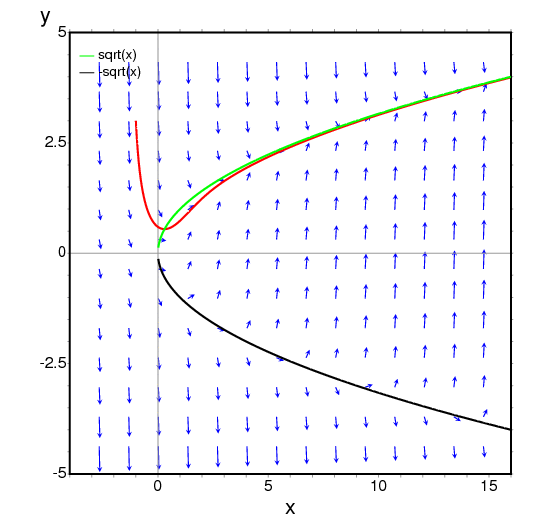
- The following example shows the direction field of a harmonic oscillator,
defined by the two equations dz/dt = v and
\(dv/dt = -kz/m,\)
and the integral curve through (z,v) = (6,0), with a slider that will allow you to change the value of m interactively (k is fixed at 2):
(%i1) plotdf([v,-k*z/m], [z,v], [parameters,"m=2,k=2"], [sliders,"m=1:5"], [trajectory_at,6,0])$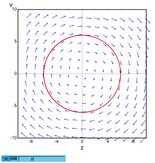
- To plot the direction field of the Duffing equation,
\(m x''+c x' + kx + bx^3 = 0,\)
we introduce the variable y=x' and use:
(%i1) plotdf([y,-(k*x + c*y + b*x^3)/m], [parameters,"k=-1,m=1.0,c=0,b=1"], [sliders,"k=-2:2,m=-1:1"],[tstep,0.1])$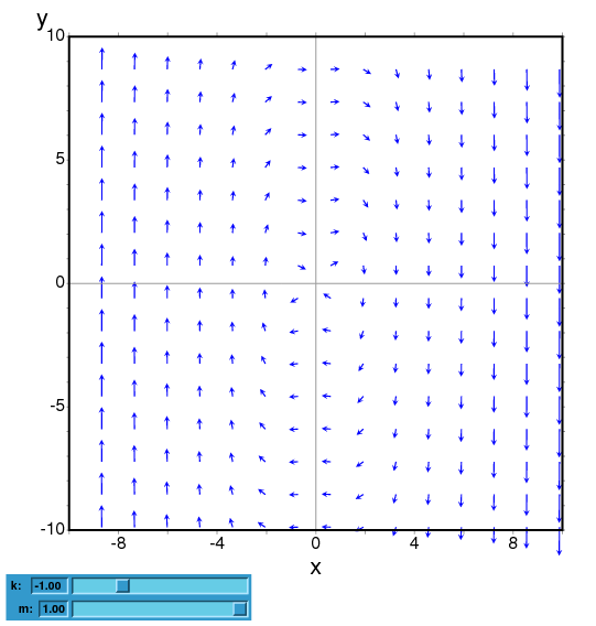
- The direction field for a damped pendulum, including the
solution for the given initial conditions, with a slider that
can be used to change the value of the mass m, and with a plot of
the two state variables as a function of time:
(%i1) plotdf([w,-g*sin(a)/l - b*w/m/l], [a,w], [parameters,"g=9.8,l=0.5,m=0.3,b=0.05"], [trajectory_at,1.05,-9],[tstep,0.01], [a,-10,2], [w,-14,14], [direction,forward], [nsteps,300], [sliders,"m=0.1:1"], [versus_t,1])$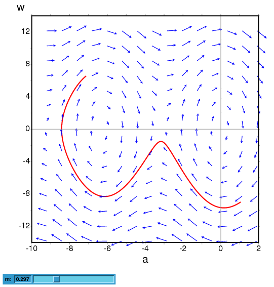
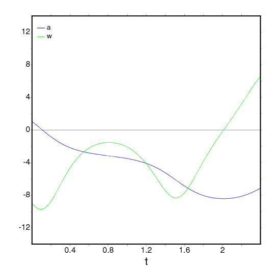
- Function: ploteq (exp, ...options...) 
-
Plots equipotential curves for exp, which should be an expression depending on two variables. The curves are obtained by integrating the differential equation that define the orthogonal trajectories to the solutions of the autonomous system obtained from the gradient of the expression given. The plot can also show the integral curves for that gradient system (option fieldlines).
This program also requires Xmaxima, even if its run from a Maxima session in a console, since the plot will be created by the Tk scripts in Xmaxima. By default, the plot region will be empty until the user clicks in a point (or gives its coordinate with in the set-up menu or via the trajectory_at option).
Most options accepted by plotdf can also be used for ploteq and the plot interface is the same that was described in plotdf.
Example:
(%i1) V: 900/((x+1)^2+y^2)^(1/2)-900/((x-1)^2+y^2)^(1/2)$ (%i2) ploteq(V,[x,-2,2],[y,-2,2],[fieldlines,"blue"])$
Clicking on a point will plot the equipotential curve that passes by that point (in red) and the orthogonal trajectory (in blue).
- Function: rk
rk (ODE, var, initial, domain)
rk ([ODE1, …, ODEm], [v1, …, vm], [init1, …, initm], domain) ¶ -
The first form solves numerically one first-order ordinary differential equation, and the second form solves a system of m of those equations, using the 4th order Runge-Kutta method. var represents the dependent variable. ODE must be an expression that depends only on the independent and dependent variables and defines the derivative of the dependent variable with respect to the independent variable.
The independent variable is specified with
domain, which must be a list of four elements as, for instance:[t, 0, 10, 0.1]
the first element of the list identifies the independent variable, the second and third elements are the initial and final values for that variable, and the last element sets the increments that should be used within that interval.
If m equations are going to be solved, there should be m dependent variables v1, v2, ..., vm. The initial values for those variables will be init1, init2, ..., initm. There will still be just one independent variable defined by
domain, as in the previous case. ODE1, ..., ODEm are the expressions that define the derivatives of each dependent variable in terms of the independent variable. The only variables that may appear in those expressions are the independent variable and any of the dependent variables. It is important to give the derivatives ODE1, ..., ODEm in the list in exactly the same order used for the dependent variables; for instance, the third element in the list will be interpreted as the derivative of the third dependent variable.The program will try to integrate the equations from the initial value of the independent variable until its last value, using constant increments. If at some step one of the dependent variables takes an absolute value too large, the integration will be interrupted at that point. The result will be a list with as many elements as the number of iterations made. Each element in the results list is itself another list with m+1 elements: the value of the independent variable, followed by the values of the dependent variables corresponding to that point.
See also
drawdf,desolveandode2.Examples:
To solve numerically the differential equation
$$ {{dx}\over{dt}} = t - x^2 $$With initial value x(t=0) = 1, in the interval of t from 0 to 8 and with increments of 0.1 for t, use:
(%i1) results: rk(t-x^2,x,1,[t,0,8,0.1])$ (%i2) plot2d ([discrete, results])$
The results will be saved in the list
resultsand the plot will show the solution obtained, with t on the horizontal axis and x on the vertical axis.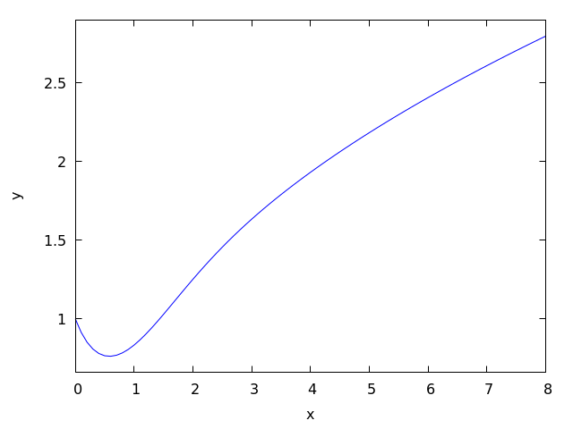
To solve numerically the system:
$$ \eqalign{ {dx\over dy} &= 4-x^2-4y^2 \cr {dy\over dt} &= y^2 - x^2 + 1 } $$for t between 0 and 4, and with values of -1.25 and 0.75 for x and y at t=0:
(%i1) sol: rk([4-x^2-4*y^2, y^2-x^2+1], [x, y], [-1.25, 0.75], [t,0,4,0.02])$(%i2) plot2d([discrete, makelist([p[1], p[3]], p, sol)], [xlabel, "t"], [ylabel, "y"])$The plot will show the solution for variable y as a function of t.
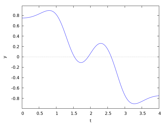 Categories: Differential equations · Numerical methods ·
Next: Sums, Products, and Series, Previous: Numerical [Contents][Index]
25 Matrices and Linear Algebra
Next: Functions and Variables for Matrices and Linear Algebra, Previous: Matrices and Linear Algebra, Up: Matrices and Linear Algebra [Contents][Index]
25.1 Introduction to Matrices and Linear Algebra
Next: Matrices, Previous: Introduction to Matrices and Linear Algebra, Up: Introduction to Matrices and Linear Algebra [Contents][Index]
25.1.1 Dot
The operator . represents noncommutative multiplication and scalar
product. When the operands are 1-column or 1-row matrices a and
b, the expression a.b is equivalent to
sum (a[i]*b[i], i, 1, length(a)). If a and b are not
complex, this is the scalar product, also called the inner product or dot
product, of a and b. The scalar product is defined as
conjugate(a).b when a and b are complex;
innerproduct in the eigen package provides the complex scalar
product.
When the operands are more general matrices,
the product is the matrix product a and b.
The number of rows of b must equal the number of columns of a,
and the result has number of rows equal to the number of rows of a
and number of columns equal to the number of columns of b.
To distinguish . as an arithmetic operator from the decimal point in a
floating point number, it may be necessary to leave spaces on either side.
For example, 5.e3 is 5000.0 but 5 . e3 is 5
times e3.
There are several flags which govern the simplification of expressions
involving ., namely dot0nscsimp, dot0simp,
dot1simp, dotassoc, dotconstrules,
dotdistrib, dotexptsimp, dotident, and
dotscrules.
Next: Vectors, Previous: Dot, Up: Introduction to Matrices and Linear Algebra [Contents][Index]
25.1.2 Matrices
Matrices are handled with speed and memory-efficiency in mind. This means that
assigning a matrix to a variable will create a reference to, not a copy of the
matrix. If the matrix is modified all references to the matrix point to the
modified object (See copymatrix for a way of avoiding this):
(%i1) M1: matrix([0,0],[0,0]);
[ 0 0 ]
(%o1) [ ]
[ 0 0 ]
(%i2) M2: M1;
[ 0 0 ]
(%o2) [ ]
[ 0 0 ]
(%i3) M1[1][1]: 2; (%o3) 2
(%i4) M2;
[ 2 0 ]
(%o4) [ ]
[ 0 0 ]
Converting a matrix to nested lists and vice versa works the following way:
(%i1) l: [[1,2],[3,4]]; (%o1) [[1, 2], [3, 4]]
(%i2) M1: apply('matrix,l);
[ 1 2 ]
(%o2) [ ]
[ 3 4 ]
(%i3) M2: transpose(M1);
[ 1 3 ]
(%o3) [ ]
[ 2 4 ]
(%i4) args(M2); (%o4) [[1, 3], [2, 4]]
Next: eigen, Previous: Matrices, Up: Introduction to Matrices and Linear Algebra [Contents][Index]
25.1.3 Vectors
vect is a package of functions for vector analysis. load ("vect")
loads this package, and demo ("vect") displays a demonstration.
The vector analysis package can combine and simplify symbolic expressions including dot products and cross products, together with the gradient, divergence, curl, and Laplacian operators. The distribution of these operators over sums or products is governed by several flags, as are various other expansions, including expansion into components in any specific orthogonal coordinate systems. There are also functions for deriving the scalar or vector potential of a field.
The vect package contains these functions:
vectorsimp, scalefactors, express,
potential, and vectorpotential.
By default the vect package does not declare the dot operator to be a
commutative operator. To get a commutative dot operator ., the command
declare(".", commutative) must be executed.
Previous: Vectors, Up: Introduction to Matrices and Linear Algebra [Contents][Index]
25.1.4 eigen
The package eigen contains several functions devoted to the
symbolic computation of eigenvalues and eigenvectors.
Maxima loads the package automatically if one of the functions
eigenvalues or eigenvectors is invoked.
The package may be loaded explicitly as load ("eigen").
demo ("eigen") displays a demonstration of the capabilities
of this package.
batch ("eigen") executes the same demonstration,
but without the user prompt between successive computations.
The functions in the eigen package are:
innerproduct, unitvector, columnvector,
gramschmidt, eigenvalues,
eigenvectors, uniteigenvectors, and
similaritytransform.
Previous: Introduction to Matrices and Linear Algebra, Up: Matrices and Linear Algebra [Contents][Index]
25.2 Functions and Variables for Matrices and Linear Algebra
- Function: addcol (M, list_1, …, list_n) 
-
Appends the column(s) given by the one or more lists (or matrices) onto the matrix M.
Categories: Matrices ·
- Function: addrow (M, list_1, …, list_n) 
-
Appends the row(s) given by the one or more lists (or matrices) onto the matrix M.
Categories: Matrices ·
- Function: adjoint (M) 
-
Returns the adjoint of the matrix M. The adjoint matrix is the transpose of the matrix of cofactors of M.
Categories: Matrices ·
- Function: augcoefmatrix ([eqn_1, …, eqn_m], [x_1, …, x_n]) 
-
Returns the augmented coefficient matrix for the variables x_1, …, x_n of the system of linear equations eqn_1, …, eqn_m. This is the coefficient matrix with a column adjoined for the constant terms in each equation (i.e., those terms not dependent upon x_1, …, x_n).
(%i1) m: [2*x - (a - 1)*y = 5*b, c + b*y + a*x = 0]$
(%i2) augcoefmatrix (m, [x, y]); [ 2 1 - a - 5 b ] (%o2) [ ] [ a b c ]Categories: Linear equations · Matrices ·
- Function: cauchy_matrix
cauchy_matrix ([x_1, x_2, …, x_m], [y_1, y_2, …, y_n])
cauchy_matrix ([x_1, x_2, …, x_n]) ¶ -
Returns a
nby m Cauchy matrix with the elements a[i,j] = 1/(x_i+y_i). The second argument ofcauchy_matrixis optional. For this case the elements of the Cauchy matrix are a[i,j] = 1/(x_i+x_j).Remark: In the literature the Cauchy matrix can be found defined in two forms. A second definition is a[i,j] = 1/(x_i-y_i).
Examples:
(%i1) cauchy_matrix([x1, x2], [y1, y2]); [ 1 1 ] [ ------- ------- ] [ y1 + x1 y2 + x1 ] (%o1) [ ] [ 1 1 ] [ ------- ------- ] [ y1 + x2 y2 + x2 ](%i2) cauchy_matrix([x1, x2]); [ 1 1 ] [ ---- ------- ] [ 2 x1 x2 + x1 ] (%o2) [ ] [ 1 1 ] [ ------- ---- ] [ x2 + x1 2 x2 ]Categories: Matrices ·
- Function: charpoly (M, x) 
-
Returns the characteristic polynomial for the matrix M with respect to variable x. That is,
determinant (M - diagmatrix (length (M), x)).(%i1) a: matrix ([3, 1], [2, 4]); [ 3 1 ] (%o1) [ ] [ 2 4 ](%i2) expand (charpoly (a, lambda)); 2 (%o2) lambda - 7 lambda + 10(%i3) (programmode: true, solve (%)); (%o3) [lambda = 5, lambda = 2]
(%i4) matrix ([x1], [x2]); [ x1 ] (%o4) [ ] [ x2 ](%i5) ev (a . % - lambda*%, %th(2)[1]); [ x2 - 2 x1 ] (%o5) [ ] [ 2 x1 - x2 ](%i6) %[1, 1] = 0; (%o6) x2 - 2 x1 = 0
(%i7) x2^2 + x1^2 = 1; 2 2 (%o7) x2 + x1 = 1(%i8) solve ([%th(2), %], [x1, x2]); 1 2 (%o8) [[x1 = - -------, x2 = - -------], sqrt(5) sqrt(5) 1 2 [x1 = -------, x2 = -------]] sqrt(5) sqrt(5)Categories: Matrices ·
- Function: coefmatrix ([eqn_1, …, eqn_m], [x_1, …, x_n]) 
-
Returns the coefficient matrix for the variables x_1, …, x_n of the system of linear equations eqn_1, …, eqn_m.
(%i1) coefmatrix([2*x-(a-1)*y+5*b = 0, b*y+a*x = 3], [x,y]); [ 2 1 - a ] (%o1) [ ] [ a b ]Categories: Linear equations · Matrices ·
- Function: col (M, i) 
-
Returns the i’th column of the matrix M. The return value is a matrix.
The matrix returned by
coldoes not share memory with the argument M; a modification to the return value does not modify M.Examples:
colreturns the i’th column of the matrix M.(%i1) abc: matrix ([12, 14, -4], [2, x, b], [3*y, -7, 9]); [ 12 14 - 4 ] [ ] (%o1) [ 2 x b ] [ ] [ 3 y - 7 9 ](%i2) col (abc, 1); [ 12 ] [ ] (%o2) [ 2 ] [ ] [ 3 y ](%i3) col (abc, 2); [ 14 ] [ ] (%o3) [ x ] [ ] [ - 7 ](%i4) col (abc, 3); [ - 4 ] [ ] (%o4) [ b ] [ ] [ 9 ]The matrix returned by
coldoes not share memory with the argument. In this example, assigning a new value toaa2does not modifyaa.(%i1) aa: matrix ([1, 2, x], [7, y, 3]); [ 1 2 x ] (%o1) [ ] [ 7 y 3 ](%i2) aa2: col (aa, 2); [ 2 ] (%o2) [ ] [ y ](%i3) aa2[2, 1]: 123; (%o3) 123
(%i4) aa2; [ 2 ] (%o4) [ ] [ 123 ](%i5) aa; [ 1 2 x ] (%o5) [ ] [ 7 y 3 ]Categories: Matrices ·
- Function: columnvector (L) 
- Function: covect (L) 
-
Returns a matrix of one column and
length (L)rows, containing the elements of the list L.covectis a synonym forcolumnvector.load ("eigen")loads this function.This is useful if you want to use parts of the outputs of the functions in this package in matrix calculations.
Example:
(%i1) load ("eigen")$(%i2) columnvector ([aa, bb, cc, dd]); [ aa ] [ ] [ bb ] (%o2) [ ] [ cc ] [ ] [ dd ]Categories: Matrices ·
- Function: copymatrix (M) 
-
Returns a copy of the matrix M. This is the only way to make a copy aside from copying M element by element.
Note that an assignment of one matrix to another, as in
m2: m1, does not copym1. An assignmentm2 [i,j]: xorsetelmx(x, i, j, m2)also modifiesm1 [i,j]. Creating a copy withcopymatrixand then using assignment creates a separate, modified copy.Categories: Matrices ·
- Function: determinant (M) 
-
Computes the determinant of M by a method similar to Gaussian elimination.
The form of the result depends upon the setting of the switch
ratmx.There is a special routine for computing sparse determinants which is called when the switches
ratmxandsparseare bothtrue.display_determinant_barsgoverns the display of determinants.Categories: Matrices ·
- Option variable: display_determinant_bars 
Default value:
trueWhen
display_determinant_barsistrue, a determinant noun expression which has a literal matrix as its sole argument is displayed with a vertical bar on either side.Otherwise,
display_determinant_barsisfalse, or the determinant is not a noun expression, or its argument is not a literal matrix; in these cases, the expression is displayed as an ordinary function call.Categories: Display flags and variables · Matrices ·
- Option variable: detout 
Default value:
falseWhen
detoutistrue, the determinant of a matrix whose inverse is computed is factored out of the inverse.For this switch to have an effect
doallmxopsanddoscmxopsshould befalse(see their descriptions). Alternatively this switch can be given toevwhich causes the other two to be set correctly.Example:
(%i1) m: matrix ([a, b], [c, d]); [ a b ] (%o1) [ ] [ c d ](%i2) detout: true$ (%i3) doallmxops: false$ (%i4) doscmxops: false$
(%i5) invert (m); [ d - b ] [ ] [ - c a ] (%o5) ------------ a d - b cCategories: Matrices · Evaluation flags ·
- Function: diagmatrix (n, x) 
-
Returns a diagonal matrix of size n by n with the diagonal elements all equal to x.
diagmatrix (n, 1)returns an identity matrix (same asident (n)).n must evaluate to an integer, otherwise
diagmatrixcomplains with an error message.x can be any kind of expression, including another matrix. If x is a matrix, it is not copied; all diagonal elements refer to the same instance, x.
Categories: Matrices ·
- Option variable: doallmxops 
Default value:
trueWhen
doallmxopsistrue, all operations relating to matrices are carried out. When it isfalsethen the setting of the individualdotswitches govern which operations are performed.Categories: Matrices ·
- Option variable: domxexpt 
Default value:
trueWhen
domxexptistrue, a matrix exponential,exp (M)where M is a matrix, is interpreted as a matrix with element[i,j]equal toexp (m[i,j]). Otherwiseexp (M)evaluates toexp (ev(M)).domxexptaffects all expressions of the formbase^powerwhere base is an expression assumed scalar or constant, and power is a list or matrix.Example:
(%i1) m: matrix ([1, %i], [a+b, %pi]); [ 1 %i ] (%o1) [ ] [ b + a %pi ](%i2) domxexpt: false$
(%i3) (1 - c)^m; [ 1 %i ] [ ] [ b + a %pi ] (%o3) (1 - c)(%i4) domxexpt: true$
(%i5) (1 - c)^m; [ %i ] [ 1 - c (1 - c) ] (%o5) [ ] [ b + a %pi ] [ (1 - c) (1 - c) ]Categories: Matrices ·
- Option variable: domxmxops 
Default value:
trueWhen
domxmxopsistrue, all matrix-matrix or matrix-list operations are carried out (but not scalar-matrix operations); if this switch isfalsesuch operations are not carried out.Categories: Matrices ·
- Option variable: domxnctimes 
Default value:
falseWhen
domxnctimesistrue, non-commutative products of matrices are carried out.Categories: Matrices ·
- Option variable: dontfactor 
Default value:
[]dontfactormay be set to a list of variables with respect to which factoring is not to occur. (The list is initially empty.) Factoring also will not take place with respect to any variables which are less important, according the variable ordering assumed for canonical rational expression (CRE) form, than those on thedontfactorlist.Categories: Expressions ·
- Option variable: doscmxops 
Default value:
falseWhen
doscmxopsistrue, scalar-matrix operations are carried out.Categories: Matrices ·
- Option variable: doscmxplus 
Default value:
falseWhen
doscmxplusistrue, scalar-matrix operations yield a matrix result. This switch is not subsumed underdoallmxops.Categories: Matrices ·
- Option variable: dot0nscsimp 
Default value:
trueWhen
dot0nscsimpistrue, a non-commutative product of zero and a nonscalar term is simplified to a commutative product.Categories: Simplification flags and variables ·
- Option variable: dot0simp 
Default value:
trueWhen
dot0simpistrue, a non-commutative product of zero and a scalar term is simplified to a commutative product.Categories: Simplification flags and variables ·
- Option variable: dot1simp 
Default value:
trueWhen
dot1simpistrue, a non-commutative product of one and another term is simplified to a commutative product.Categories: Simplification flags and variables ·
- Option variable: dotassoc 
Default value:
trueWhen
dotassocistrue, an expression(A.B).Csimplifies toA.(B.C).Categories: Simplification flags and variables ·
- Option variable: dotconstrules 
Default value:
trueWhen
dotconstrulesistrue, a non-commutative product of a constant and another term is simplified to a commutative product. Turning on this flag effectively turns ondot0simp,dot0nscsimp, anddot1simpas well.Categories: Simplification flags and variables ·
- Option variable: dotdistrib 
Default value:
falseWhen
dotdistribistrue, an expressionA.(B + C)simplifies toA.B + A.C.Categories: Simplification flags and variables ·
- Option variable: dotexptsimp 
Default value:
trueWhen
dotexptsimpistrue, an expressionA.Asimplifies toA^^2.Categories: Simplification flags and variables ·
- Option variable: dotident 
Default value: 1
dotidentis the value returned byX^^0.Categories: Simplification flags and variables ·
- Option variable: dotscrules 
Default value:
falseWhen
dotscrulesistrue, an expressionA.SCorSC.Asimplifies toSC*AandA.(SC*B)simplifies toSC*(A.B).Categories: Simplification flags and variables ·
- Function: echelon (M) 
-
Returns the echelon form of the matrix M, as produced by Gaussian elimination. The echelon form is computed from M by elementary row operations such that the first non-zero element in each row in the resulting matrix is one and the column elements under the first one in each row are all zero.
triangularizealso carries out Gaussian elimination, but it does not normalize the leading non-zero element in each row.lu_factorandcholeskyare other functions which yield triangularized matrices.(%i1) M: matrix ([3, 7, aa, bb], [-1, 8, 5, 2], [9, 2, 11, 4]); [ 3 7 aa bb ] [ ] (%o1) [ - 1 8 5 2 ] [ ] [ 9 2 11 4 ](%i2) echelon (M); [ 1 - 8 - 5 - 2 ] [ ] [ 28 11 ] [ 0 1 -- -- ] (%o2) [ 37 37 ] [ ] [ 37 bb - 119 ] [ 0 0 1 ----------- ] [ 37 aa - 313 ]Categories: Linear equations · Matrices ·
- Function: eigenvalues (M) 
- Function: eivals (M) 
-
Returns a list of two lists containing the eigenvalues of the matrix M. The first sublist of the return value is the list of eigenvalues of the matrix, and the second sublist is the list of the multiplicities of the eigenvalues in the corresponding order.
eivalsis a synonym foreigenvalues.eigenvaluescalls the functionsolveto find the roots of the characteristic polynomial of the matrix. Sometimessolvemay not be able to find the roots of the polynomial; in that case some other functions in this package (exceptinnerproduct,unitvector,columnvectorandgramschmidt) will not work. Sometimessolvemay find only a subset of the roots of the polynomial. This may happen when the factoring of the polynomial contains polynomials of degree 5 or more. In such cases a warning message is displayed and the only the roots found and their corresponding multiplicities are returned.In some cases the eigenvalues found by
solvemay be complicated expressions. (This may happen whensolvereturns a not-so-obviously real expression for an eigenvalue which is known to be real.) It may be possible to simplify the eigenvalues using some other functions.The package
eigen.macis loaded automatically wheneigenvaluesoreigenvectorsis referenced. Ifeigen.macis not already loaded,load ("eigen")loads it. After loading, all functions and variables in the package are available.For matrices consisting of only floating-point values, see also
dgeev.Categories: Package eigen ·
- Function: eigenvectors (M) 
- Function: eivects (M) 
-
Computes eigenvectors of the matrix M. The return value is a list of two elements. The first is a list of the eigenvalues of M and a list of the multiplicities of the eigenvalues. The second is a list of lists of eigenvectors. There is one list of eigenvectors for each eigenvalue. There may be one or more eigenvectors in each list.
eivectsis a synonym foreigenvectors.The package
eigen.macis loaded automatically wheneigenvaluesoreigenvectorsis referenced. Ifeigen.macis not already loaded,load ("eigen")loads it. After loading, all functions and variables in the package are available.Note that
eigenvectorsinternally callseigenvaluesto obtain eigenvalues. So, wheneigenvaluesreturns a subset of all the eigenvalues, theeigenvectorsreturns the corresponding subset of the all the eigenvectors, with the same warning displayed aseigenvalues.The flags that affect this function are:
nondiagonalizableis set totrueorfalsedepending on whether the matrix is nondiagonalizable or diagonalizable aftereigenvectorsreturns.hermitianmatrixwhentrue, causes the degenerate eigenvectors of the Hermitian matrix to be orthogonalized using the Gram-Schmidt algorithm.knowneigvalswhentruecauses theeigenpackage to assume the eigenvalues of the matrix are known to the user and stored under the global namelisteigvals.listeigvalsshould be set to a list similar to the outputeigenvalues.The function
algsysis used here to solve for the eigenvectors. Sometimes if the eigenvalues are messy,algsysmay not be able to find a solution. In some cases, it may be possible to simplify the eigenvalues by first finding them usingeigenvaluescommand and then using other functions to reduce them to something simpler. Following simplification,eigenvectorscan be called again with theknowneigvalsflag set totrue.See also
eigenvalues.For matrices consisting of only floating-point values, see also
dgeev.Examples:
A matrix which has just one eigenvector per eigenvalue.
(%i1) M1: matrix ([11, -1], [1, 7]); [ 11 - 1 ] (%o1) [ ] [ 1 7 ](%i2) [vals, vecs] : eigenvectors (M1); (%o2) [[[9 - sqrt(3), sqrt(3) + 9], [1, 1]], [[[1, sqrt(3) + 2]], [[1, 2 - sqrt(3)]]]](%i3) for i thru length (vals[1]) do disp (val[i] = vals[1][i], mult[i] = vals[2][i], vec[i] = vecs[i]); val = 9 - sqrt(3) 1 mult = 1 1 vec = [[1, sqrt(3) + 2]] 1 val = sqrt(3) + 9 2 mult = 1 2 vec = [[1, 2 - sqrt(3)]] 2 (%o3) doneA matrix which has two eigenvectors for one eigenvalue (namely 2).
(%i1) M1 : matrix ([0, 1, 0, 0], [0, 0, 0, 0], [0, 0, 2, 0], [0, 0, 0, 2]); [ 0 1 0 0 ] [ ] [ 0 0 0 0 ] (%o1) [ ] [ 0 0 2 0 ] [ ] [ 0 0 0 2 ](%i2) [vals, vecs] : eigenvectors (M1); (%o2) [[[0, 2], [2, 2]], [[[1, 0, 0, 0]], [[0, 0, 1, 0], [0, 0, 0, 1]]]](%i3) for i thru length (vals[1]) do disp (val[i] = vals[1][i], mult[i] = vals[2][i], vec[i] = vecs[i]); val = 0 1 mult = 2 1 vec = [[1, 0, 0, 0]] 1 val = 2 2 mult = 2 2 vec = [[0, 0, 1, 0], [0, 0, 0, 1]] 2 (%o3) doneCategories: Package eigen ·
- Function: ematrix (m, n, x, i, j) 
-
Returns an m by n matrix, all elements of which are zero except for the
[i, j]element which is x.Categories: Matrices ·
- Function: entermatrix (m, n) 
-
Returns an m by n matrix, reading the elements interactively.
If n is equal to m, Maxima prompts for the type of the matrix (diagonal, symmetric, antisymmetric, or general) and for each element. Each response is terminated by a semicolon
;or dollar sign$.If n is not equal to m, Maxima prompts for each element.
The elements may be any expressions, which are evaluated.
entermatrixevaluates its arguments.(%i1) n: 3$ (%i2) m: entermatrix (n, n)$ Is the matrix 1. Diagonal 2. Symmetric 3. Antisymmetric 4. General Answer 1, 2, 3 or 4 : 1$ Row 1 Column 1: (a+b)^n$ Row 2 Column 2: (a+b)^(n+1)$ Row 3 Column 3: (a+b)^(n+2)$ Matrix entered. (%i3) m; [ 3 ] [ (b + a) 0 0 ] [ ] (%o3) [ 4 ] [ 0 (b + a) 0 ] [ ] [ 5 ] [ 0 0 (b + a) ]Categories: Console interaction · Matrices ·
- Function: genmatrix
genmatrix (a, i_2, j_2, i_1, j_1)
genmatrix (a, i_2, j_2, i_1)
genmatrix (a, i_2, j_2) ¶ -
Returns a matrix generated from a, taking element
a[i_1, j_1]as the upper-left element anda[i_2, j_2]as the lower-right element of the matrix. Here a is a declared array (created byarraybut not bymake_array) or ahashed array, or amemoizing function, or a lambda expression of two arguments. (Amemoizing functionis created like other functions with:=ordefine, but arguments are enclosed in square brackets instead of parentheses.)If j_1 is omitted, it is assumed equal to i_1. If both j_1 and i_1 are omitted, both are assumed equal to 1.
If a selected element
i,jof the array is undefined, the matrix will contain a symbolic elementa[i,j].Examples:
(%i1) h [i, j] := 1 / (i + j - 1); 1 (%o1) h := --------- i, j i + j - 1(%i2) genmatrix (h, 3, 3); [ 1 1 ] [ 1 - - ] [ 2 3 ] [ ] [ 1 1 1 ] (%o2) [ - - - ] [ 2 3 4 ] [ ] [ 1 1 1 ] [ - - - ] [ 3 4 5 ](%i3) array (a, fixnum, 2, 2); (%o3) a
(%i4) a [1, 1] : %e; (%o4) %e
(%i5) a [2, 2] : %pi; (%o5) %pi
(%i6) genmatrix (a, 2, 2); [ %e 0 ] (%o6) [ ] [ 0 %pi ](%i7) genmatrix (lambda ([i, j], j - i), 3, 3); [ 0 1 2 ] [ ] (%o7) [ - 1 0 1 ] [ ] [ - 2 - 1 0 ](%i8) genmatrix (B, 2, 2); [ B B ] [ 1, 1 1, 2 ] (%o8) [ ] [ B B ] [ 2, 1 2, 2 ]Categories: Matrices ·
- Function: gramschmidt
gramschmidt (x)
gramschmidt (x, F) ¶ -
Carries out the Gram-Schmidt orthogonalization algorithm on x, which is either a matrix or a list of lists. x is not modified by
gramschmidt. The inner product employed bygramschmidtis F, if present, otherwise the inner product is the functioninnerproduct.If x is a matrix, the algorithm is applied to the rows of x. If x is a list of lists, the algorithm is applied to the sublists, which must have equal numbers of elements. In either case, the return value is a list of lists, the sublists of which are orthogonal and span the same space as x. If the dimension of the span of x is less than the number of rows or sublists, some sublists of the return value are zero.
factoris called at each stage of the algorithm to simplify intermediate results. As a consequence, the return value may contain factored integers.load("eigen")loads this function.Example:
Gram-Schmidt algorithm using default inner product function.
(%i1) load ("eigen")$(%i2) x: matrix ([1, 2, 3], [9, 18, 30], [12, 48, 60]); [ 1 2 3 ] [ ] (%o2) [ 9 18 30 ] [ ] [ 12 48 60 ](%i3) y: gramschmidt (x); 2 2 4 3 3 3 3 5 2 3 2 3 (%o3) [[1, 2, 3], [- ---, - --, ---], [- ----, ----, 0]] 2 7 7 2 7 5 5(%i4) map (innerproduct, [y[1], y[2], y[3]], [y[2], y[3], y[1]]); (%o4) [0, 0, 0]
Gram-Schmidt algorithm using a specified inner product function.
(%i1) load ("eigen")$(%i2) ip (f, g) := integrate (f * g, u, a, b); (%o2) ip(f, g) := integrate(f g, u, a, b)
(%i3) y: gramschmidt ([1, sin(u), cos(u)], ip), a=-%pi/2, b=%pi/2; %pi cos(u) - 2 (%o3) [1, sin(u), --------------] %pi(%i4) map (ip, [y[1], y[2], y[3]], [y[2], y[3], y[1]]), a=-%pi/2, b=%pi/2; (%o4) [0, 0, 0]Categories: Package eigen ·
- Function: innerproduct (x, y) 
- Function: inprod (x, y) 
-
Returns the inner product (also called the scalar product or dot product) of x and y, which are lists of equal length, or both 1-column or 1-row matrices of equal length. The return value is
conjugate (x) . y, where.is the noncommutative multiplication operator.load ("eigen")loads this function.inprodis a synonym forinnerproduct.Categories: Package eigen ·
- Function: invert_by_adjoint (M) 
Returns the inverse of the matrix M. The inverse is computed by the adjoint method.
invert_by_adjointhonors theratmxanddetoutflags, the same asinvert.
- Function: invert (M) 
-
Returns the inverse of the matrix M. The inverse is computed via the LU decomposition.
When
ratmxistrue, elements of M are converted to canonical rational expressions (CRE), and the elements of the return value are also CRE.When
ratmxisfalse, elements of M are not converted to a common representation. In particular, float and bigfloat elements are not converted to rationals.When
detoutistrue, the determinant is factored out of the inverse. The global flagsdoallmxopsanddoscmxopsmust befalseto prevent the determinant from being absorbed into the inverse.xthrucan multiply the determinant into the inverse.invertdoes not apply any simplifications to the elements of the inverse apart from the default arithmetic simplifications.ratsimpandexpandcan apply additional simplifications. In particular, when M has polynomial elements,expand(invert(M))might be preferable.invert(M)is equivalent toM^^-1.Categories: Matrices ·
- Function: list_matrix_entries (M) 
-
Returns a list containing the elements of the matrix M.
Example:
(%i1) list_matrix_entries(matrix([a,b],[c,d])); (%o1) [a, b, c, d]
Categories: Matrices ·
- Option variable: lmxchar 
Default value:
[lmxcharis the character displayed as the left delimiter of a matrix. See alsormxchar.lmxcharis only used whendisplay2d_unicodeisfalse.Example:
(%i1) display2d_unicode: false $ (%i2) lmxchar: "|"$
(%i3) matrix ([a, b, c], [d, e, f], [g, h, i]); | a b c ] | ] (%o3) | d e f ] | ] | g h i ]Categories: Display flags and variables · Matrices ·
- Option variable: display_matrix_brackets 
Default value:
trueWhen
display_matrix_bracketsistrue, matrices are displayed with brackets (square braces) to the left and right.When
display_matrix_bracketsisfalse, matrices are not displayed with brackets; only the matrix elements are displayed.Categories: Matrices · Display flags and variables ·
- Option variable: display_matrix_padding_horizontal 
Default value:
trueWhen
display_matrix_padding_horizontalistrue, matrices are displayed with spaces between successive columns, and a space before the first column and a space after the last column.When
display_matrix_padding_horizontalisfalse, matrices are not displayed with spaces between successive columns, and no space before the first column and no space after the last column. Successive columns are immediately adjacent to each other, and the first column is immediately adjacent to the left bracket, and the last column is immediately adjacent to the right bracket, if the brackets are present (seedisplay_matrix_brackets).See also
display_matrix_padding_vertical.Examples:
(%i1) display_matrix_padding_horizontal; (%o1) true (%i2) foo: matrix ([a, b, c], [d, e, f], [g, h, i]); ┌ ┐ │ a b c │ │ │ (%o2) │ d e f │ │ │ │ g h i │ └ ┘(%i3) display_matrix_padding_horizontal: false; (%o3) false (%i4) foo; ┌ ┐ │abc│ │ │ (%o4) │def│ │ │ │ghi│ └ ┘Categories: Matrices · Display flags and variables ·
- Option variable: display_matrix_padding_vertical 
Default value:
trueWhen
display_matrix_padding_verticalistrue, matrices are displayed with an empty line between successive rows.When
display_matrix_padding_verticalisfalse, matrices are not displayed with an empty line between successive rows; successive rows are immediately adjacent to each other.See also
display_matrix_padding_horizontal.Examples:
(%i1) display_matrix_padding_vertical; (%o1) true (%i2) foo: matrix ([a, b, c], [d, e, f], [g, h, i]); ┌ ┐ │ a b c │ │ │ (%o2) │ d e f │ │ │ │ g h i │ └ ┘(%i3) display_matrix_padding_vertical: false; (%o3) false (%i4) foo; ┌ ┐ │ a b c │ (%o4) │ d e f │ │ g h i │ └ ┘Categories: Matrices · Display flags and variables ·
- Function: matrix (row_1, …, row_n) 
-
Returns a rectangular matrix which has the rows row_1, …, row_n. Each row is a list of expressions. All rows must be the same length.
The operations
+(addition),-(subtraction),*(multiplication), and/(division), are carried out element by element when the operands are two matrices, a scalar and a matrix, or a matrix and a scalar. The operation^(exponentiation, equivalently**) is carried out element by element if the operands are a scalar and a matrix or a matrix and a scalar, but not if the operands are two matrices. All operations are normally carried out in full, including.(noncommutative multiplication).Matrix multiplication is represented by the noncommutative multiplication operator
.. The corresponding noncommutative exponentiation operator is^^. For a matrixA,A.A = A^^2andA^^-1is the inverse of A, if it exists.A^^-1is equivalent toinvert(A).There are switches for controlling simplification of expressions involving dot and matrix-list operations. These are
doallmxops,domxexpt,domxmxops,doscmxops, anddoscmxplus.There are additional options which are related to matrices. These are:
lmxchar,rmxchar,ratmx,listarith,detout,scalarmatrixandsparse.There are a number of functions which take matrices as arguments or yield matrices as return values. See
eigenvalues,eigenvectors,determinant,charpoly,genmatrix,addcol,addrow,copymatrix,transpose,echelon, andrank.Option variables
display_matrix_bracketsanddisplay_matrix_padding_verticalgovern the display of matrices.Examples:
- Construction of matrices from lists.
(%i1) x: matrix ([17, 3], [-8, 11]); [ 17 3 ] (%o1) [ ] [ - 8 11 ](%i2) y: matrix ([%pi, %e], [a, b]); [ %pi %e ] (%o2) [ ] [ a b ]- Addition, element by element.
(%i3) x + y; [ %pi + 17 %e + 3 ] (%o3) [ ] [ a - 8 b + 11 ]- Subtraction, element by element.
(%i4) x - y; [ 17 - %pi 3 - %e ] (%o4) [ ] [ - a - 8 11 - b ]- Multiplication, element by element.
(%i5) x * y; [ 17 %pi 3 %e ] (%o5) [ ] [ - 8 a 11 b ]- Division, element by element.
(%i6) x / y; [ 17 - 1 ] [ --- 3 %e ] [ %pi ] (%o6) [ ] [ 8 11 ] [ - - -- ] [ a b ]- Matrix to a scalar exponent, element by element.
(%i7) x ^ 3; [ 4913 27 ] (%o7) [ ] [ - 512 1331 ]- Scalar base to a matrix exponent, element by element.
(%i8) exp(y); [ %pi %e ] [ %e %e ] (%o8) [ ] [ a b ] [ %e %e ]- Matrix base to a matrix exponent. This is not carried out element by element.
See also
matrixexp.
(%i9) x ^ y; [ %pi %e ] [ ] [ a b ] [ 17 3 ] (%o9) [ ] [ - 8 11 ]- Noncommutative matrix multiplication.
(%i10) x . y; [ 3 a + 17 %pi 3 b + 17 %e ] (%o10) [ ] [ 11 a - 8 %pi 11 b - 8 %e ] (%i11) y . x; [ 17 %pi - 8 %e 3 %pi + 11 %e ] (%o11) [ ] [ 17 a - 8 b 11 b + 3 a ]- Noncommutative matrix exponentiation.
A scalar base b to a matrix power M
is carried out element by element and so
b^^mis the same asb^m.
(%i12) x ^^ 3; [ 3833 1719 ] (%o12) [ ] [ - 4584 395 ] (%i13) %e ^^ y;[ %pi %e ] [ %e %e ] (%o13) [ ] [ a b ] [ %e %e ]- A matrix raised to a -1 exponent with noncommutative exponentiation is the matrix inverse, if it exists.
(%i14) x ^^ -1; [ 11 3 ] [ --- - --- ] [ 211 211 ] (%o14) [ ] [ 8 17 ] [ --- --- ] [ 211 211 ] (%i15) x . (x ^^ -1); [ 1 0 ] (%o15) [ ] [ 0 1 ]Categories: Matrices ·
- Function: matrixexp
matrixexp (M)
matrixexp (M, n)
matrixexp (M, V) ¶ -
Calculates the matrix exponential \(e^{M\cdot V}\) . Instead of the vector V a number n can be specified as the second argument. If this argument is omitted
matrixexpreplaces it by1.The matrix exponential of a matrix M can be expressed as a power series: $$ e^M=\sum_{k=0}^\infty{\left(\frac{M^k}{k!}\right)} $$
Categories: Matrices ·
- Function: matrixmap (f, M) 
-
Returns a matrix with element
i,jequal tof(M[i,j]).See also
map,fullmap,fullmapl, andapply.Categories: Matrices ·
- Function: matrixp (expr) 
-
Returns
trueif expr is a matrix, otherwisefalse.Categories: Predicate functions · Matrices ·
- Option variable: matrix_element_add 
Default value:
+matrix_element_addis the operation invoked in place of addition in a matrix multiplication.matrix_element_addcan be assigned any n-ary operator (that is, a function which handles any number of arguments). The assigned value may be the name of an operator enclosed in quote marks, the name of a function, or a lambda expression.See also
matrix_element_multandmatrix_element_transpose.Example:
(%i1) matrix_element_add: "*"$ (%i2) matrix_element_mult: "^"$
(%i3) aa: matrix ([a, b, c], [d, e, f]); [ a b c ] (%o3) [ ] [ d e f ](%i4) bb: matrix ([u, v, w], [x, y, z]); [ u v w ] (%o4) [ ] [ x y z ](%i5) aa . transpose (bb); [ u v w x y z ] [ a b c a b c ] (%o5) [ ] [ u v w x y z ] [ d e f d e f ]Categories: Matrices ·
- Option variable: matrix_element_mult 
Default value:
*matrix_element_multis the operation invoked in place of multiplication in a matrix multiplication.matrix_element_multcan be assigned any binary operator. The assigned value may be the name of an operator enclosed in quote marks, the name of a function, or a lambda expression.The dot operator
.is a useful choice in some contexts.See also
matrix_element_addandmatrix_element_transpose.Example:
(%i1) matrix_element_add: lambda ([[x]], sqrt (apply ("+", x)))$ (%i2) matrix_element_mult: lambda ([x, y], (x - y)^2)$(%i3) [a, b, c] . [x, y, z]; 2 2 2 (%o3) sqrt((c - z) + (b - y) + (a - x) )(%i4) aa: matrix ([a, b, c], [d, e, f]); [ a b c ] (%o4) [ ] [ d e f ](%i5) bb: matrix ([u, v, w], [x, y, z]); [ u v w ] (%o5) [ ] [ x y z ](%i6) aa . transpose (bb); [ 2 2 2 ] [ sqrt((c - w) + (b - v) + (a - u) ) ] (%o6) Col 1 = [ ] [ 2 2 2 ] [ sqrt((f - w) + (e - v) + (d - u) ) ] [ 2 2 2 ] [ sqrt((c - z) + (b - y) + (a - x) ) ] Col 2 = [ ] [ 2 2 2 ] [ sqrt((f - z) + (e - y) + (d - x) ) ]Categories: Matrices ·
- Option variable: matrix_element_transpose 
Default value:
falsematrix_element_transposeis the operation applied to each element of a matrix when it is transposed.matrix_element_multcan be assigned any unary operator. The assigned value may be the name of an operator enclosed in quote marks, the name of a function, or a lambda expression.When
matrix_element_transposeequalstranspose, thetransposefunction is applied to every element. Whenmatrix_element_transposeequalsnonscalars, thetransposefunction is applied to every nonscalar element. If some element is an atom, thenonscalarsoption appliestransposeonly if the atom is declared nonscalar, while thetransposeoption always appliestranspose.The default value,
false, means no operation is applied.See also
matrix_element_addandmatrix_element_mult.Examples:
(%i1) declare (a, nonscalar)$
(%i2) transpose ([a, b]); [ a ] (%o2) [ ] [ b ](%i3) matrix_element_transpose: nonscalars$
(%i4) transpose ([a, b]); [ transpose(a) ] (%o4) [ ] [ b ](%i5) matrix_element_transpose: transpose$
(%i6) transpose ([a, b]); [ transpose(a) ] (%o6) [ ] [ transpose(b) ](%i7) matrix_element_transpose: lambda ([x], realpart(x) - %i*imagpart(x))$
(%i8) m: matrix ([1 + 5*%i, 3 - 2*%i], [7*%i, 11]); [ 5 %i + 1 3 - 2 %i ] (%o8) [ ] [ 7 %i 11 ](%i9) transpose (m); [ 1 - 5 %i - 7 %i ] (%o9) [ ] [ 2 %i + 3 11 ]Categories: Matrices ·
- Function: mattrace (M) 
-
Returns the trace (that is, the sum of the elements on the main diagonal) of the square matrix M.
mattraceis called byncharpoly, an alternative to Maxima’scharpoly.load ("nchrpl")loads this function.Categories: Matrices · Package nchrpl ·
- Function: minor (M, i, j) 
-
Returns the i, j minor of the matrix M. That is, M with row i and column j removed.
Categories: Matrices ·
- Function: ncharpoly (M, x) 
-
Returns the characteristic polynomial of the matrix M with respect to x. This is an alternative to Maxima’s
charpoly.ncharpolyworks by computing traces of powers of the given matrix, which are known to be equal to sums of powers of the roots of the characteristic polynomial. From these quantities the symmetric functions of the roots can be calculated, which are nothing more than the coefficients of the characteristic polynomial.charpolyworks by forming the determinant ofx * ident [n] - a. Thusncharpolywins, for example, in the case of large dense matrices filled with integers, since it avoids polynomial arithmetic altogether.load ("nchrpl")loads this file.Categories: Matrices · Package nchrpl ·
- Function: newdet (M) 
-
Computes the determinant of the matrix M by the Johnson-Gentleman tree minor algorithm.
newdetreturns the result in CRE form.Categories: Matrices ·
- Function: permanent (M) 
-
Computes the permanent of the matrix M by the Johnson-Gentleman tree minor algorithm. A permanent is like a determinant but with no sign changes.
permanentreturns the result in CRE form.See also
newdet.Categories: Matrices ·
- Function: rank (M) 
-
Computes the rank of the matrix M. That is, the order of the largest non-singular subdeterminant of M.
rank may return the wrong answer if it cannot determine that a matrix element that is equivalent to zero is indeed so.
Categories: Matrices ·
- Option variable: ratmx 
Default value:
falseWhen
ratmxisfalse, determinant and matrix addition, subtraction, and multiplication are performed in the representation of the matrix elements and cause the result of matrix inversion to be left in general representation.When
ratmxistrue, the 4 operations mentioned above are performed in CRE form and the result of matrix inverse is in CRE form. Note that this may cause the elements to be expanded (depending on the setting ofratfac) which might not always be desired.Categories: Matrices · Rational expressions ·
- Function: row (M, i) 
-
Returns the i’th row of the matrix M. The return value is a matrix.
The matrix returned by
rowshares memory with the argument M; a modification to the return value modifies M.Examples:
rowreturns the i’th row of the matrix M.(%i1) abc: matrix ([12, 14, -4], [2, x, b], [3*y, -7, 9]); [ 12 14 - 4 ] [ ] (%o1) [ 2 x b ] [ ] [ 3 y - 7 9 ](%i2) row (abc, 1); (%o2) [ 12 14 - 4 ]
(%i3) row (abc, 2); (%o3) [ 2 x b ]
(%i4) row (abc, 3); (%o4) [ 3 y - 7 9 ]
The matrix returned by
rowshares memory with the argument. In this example, assigning a new value toaa2also modifiesaa.(%i1) aa: matrix ([1, 2, x], [7, y, 3]); [ 1 2 x ] (%o1) [ ] [ 7 y 3 ](%i2) aa2: row (aa, 2); (%o2) [ 7 y 3 ]
(%i3) aa2[1, 3]: 123; (%o3) 123
(%i4) aa2; (%o4) [ 7 y 123 ]
(%i5) aa; [ 1 2 x ] (%o5) [ ] [ 7 y 123 ]Categories: Matrices ·
- Option variable: rmxchar 
Default value:
]rmxcharis the character drawn on the right-hand side of a matrix.rmxcharis only used whendisplay2d_unicodeisfalse.See also
lmxchar.Categories: Display flags and variables ·
- Option variable: scalarmatrixp 
Default value:
trueWhen
scalarmatrixpistrue, then whenever a 1 x 1 matrix is produced as a result of computing the dot product of matrices it is simplified to a scalar, namely the sole element of the matrix.When
scalarmatrixpisall, then all 1 x 1 matrices are simplified to scalars.When
scalarmatrixpisfalse, 1 x 1 matrices are not simplified to scalars.Categories: Matrices · Simplification flags and variables ·
- Function: scalefactors (coordinatetransform) 
-
Here the argument coordinatetransform evaluates to the form
[[expression1, expression2, ...], indeterminate1, indeterminat2, ...], where the variables indeterminate1, indeterminate2, etc. are the curvilinear coordinate variables and where a set of rectangular Cartesian components is given in terms of the curvilinear coordinates by[expression1, expression2, ...].coordinatesis set to the vector[indeterminate1, indeterminate2,...], anddimensionis set to the length of this vector. SF[1], SF[2], …, SF[DIMENSION] are set to the coordinate scale factors, andsfprodis set to the product of these scale factors. Initially,coordinatesis[X, Y, Z],dimensionis 3, and SF[1]=SF[2]=SF[3]=SFPROD=1, corresponding to 3-dimensional rectangular Cartesian coordinates. To expand an expression into physical components in the current coordinate system, there is a function with usage of the formCategories: Package vect ·
- Function: setelmx (x, i, j, M) 
-
Assigns x to the (i, j)’th element of the matrix M, and returns the altered matrix.
M [i, j]: xhas the same effect, but returns x instead of M.Categories: Matrices ·
- Function: similaritytransform (M) 
- Function: simtran (M) 
-
similaritytransformcomputes a similarity transform of the matrixM. It returns a list which is the output of theuniteigenvectorscommand. In addition if the flagnondiagonalizableisfalsetwo global matricesleftmatrixandrightmatrixare computed. These matrices have the property thatleftmatrix . M . rightmatrixis a diagonal matrix with the eigenvalues of M on the diagonal. Ifnondiagonalizableistruethe left and right matrices are not computed.If the flag
hermitianmatrixistruethenleftmatrixis the complex conjugate of the transpose ofrightmatrix. Otherwiseleftmatrixis the inverse ofrightmatrix.rightmatrixis the matrix the columns of which are the unit eigenvectors of M. The other flags (seeeigenvaluesandeigenvectors) have the same effects sincesimilaritytransformcalls the other functions in the package in order to be able to formrightmatrix.load ("eigen")loads this function.simtranis a synonym forsimilaritytransform.Categories: Package eigen ·
- Option variable: sparse 
Default value:
falseWhen
sparseistrue, and ifratmxistrue, thendeterminantwill use special routines for computing sparse determinants.Categories: Matrices ·
- Function: submatrix
submatrix (i_1, …, i_m, M, j_1, …, j_n)
submatrix (i_1, …, i_m, M)
submatrix (M, j_1, …, j_n) ¶ -
Returns a new matrix composed of the matrix M with rows i_1, …, i_m deleted, and columns j_1, …, j_n deleted.
Categories: Matrices ·
- Function: transpose (M) 
-
Returns the transpose of M.
If M is a matrix, the return value is another matrix N such that
N[i,j] = M[j,i].If M is a list, the return value is a matrix N of
length (m)rows and 1 column, such thatN[i,1] = M[i].Otherwise M is a symbol, and the return value is a noun expression
'transpose (M).Categories: Matrices ·
- Function: triangularize (M) 
-
Returns the upper triangular form of the matrix
M, as produced by Gaussian elimination. The return value is the same asechelon, except that the leading nonzero coefficient in each row is not normalized to 1.lu_factorandcholeskyare other functions which yield triangularized matrices.(%i1) M: matrix ([3, 7, aa, bb], [-1, 8, 5, 2], [9, 2, 11, 4]); [ 3 7 aa bb ] [ ] (%o1) [ - 1 8 5 2 ] [ ] [ 9 2 11 4 ](%i2) triangularize (M); [ - 1 8 5 2 ] [ ] (%o2) [ 0 - 74 - 56 - 22 ] [ ] [ 0 0 626 - 74 aa 238 - 74 bb ]Categories: Linear equations · Matrices ·
- Function: uniteigenvectors (M) 
- Function: ueivects (M) 
-
Computes unit eigenvectors of the matrix M. The return value is a list of lists, the first sublist of which is the output of the
eigenvaluescommand, and the other sublists of which are the unit eigenvectors of the matrix corresponding to those eigenvalues respectively.The flags mentioned in the description of the
eigenvectorscommand have the same effects in this one as well.When
knowneigvectsistrue, theeigenpackage assumes that the eigenvectors of the matrix are known to the user and are stored under the global namelisteigvects.listeigvectsshould be set to a list similar to the output of theeigenvectorscommand.If
knowneigvectsis set totrueand the list of eigenvectors is given the setting of the flagnondiagonalizablemay not be correct. If that is the case please set it to the correct value. The author assumes that the user knows what he is doing and will not try to diagonalize a matrix the eigenvectors of which do not span the vector space of the appropriate dimension.load ("eigen")loads this function.ueivectsis a synonym foruniteigenvectors.Categories: Package eigen ·
- Function: unitvector (x) 
- Function: uvect (x) 
-
Returns x/norm(x); this is a unit vector in the same direction as x.
load ("eigen")loads this function.uvectis a synonym forunitvector.Categories: Package eigen ·
- Function: vectorpotential (givencurl) 
-
Returns the vector potential of a given curl vector, in the current coordinate system.
potentialzerolochas a similar role as forpotential, but the order of the left-hand sides of the equations must be a cyclic permutation of the coordinate variables.Categories: Package vect ·
- Function: vectorsimp (expr) 
-
Applies simplifications and expansions according to the following global flags:
expandall,expanddot,expanddotplus,expandcross,expandcrossplus,expandcrosscross,expandgrad,expandgradplus,expandgradprod,expanddiv,expanddivplus,expanddivprod,expandcurl,expandcurlplus,expandcurlcurl,expandlaplacian,expandlaplacianplus, andexpandlaplacianprod.All these flags have default value
false. Theplussuffix refers to employing additivity or distributivity. Theprodsuffix refers to the expansion for an operand that is any kind of product.expandcrosscrossSimplifies \(p \sim (q \sim r)\) to \((p . r)q - (p . q)r.\)
expandcurlcurlSimplifies \({\rm curl}\; {\rm curl}\; p\) to \({\rm grad}\; {\rm div}\; p + {\rm div}\; {\rm grad}\; p.\)
expandlaplaciantodivgradSimplifies \({\rm laplacian}\; p\) to \({\rm div}\; {\rm grad}\; p.\)
expandcrossEnables
expandcrossplusandexpandcrosscross.expandplusEnables
expanddotplus,expandcrossplus,expandgradplus,expanddivplus,expandcurlplus, andexpandlaplacianplus.expandprodEnables
expandgradprod,expanddivprod, andexpandlaplacianprod.
These flags have all been declared
evflag.Categories: Package vect · Simplification functions ·
- Option variable: vect_cross 
Default value:
falseWhen
vect_crossistrue, it allows DIFF(X~Y,T) to work where ~ is defined in SHARE;VECT (where VECT_CROSS is set totrue, anyway.)Categories: Package vect · Differential calculus ·
- Function: zeromatrix (m, n) 
-
Returns an m by n matrix, all elements of which are zero.
Categories: Matrices ·
Next: Number Theory, Previous: Matrices and Linear Algebra [Contents][Index]
26 Sums, Products, and Series
- Functions and Variables for Sums and Products
- Introduction to Series
- Functions and Variables for Series
- Introduction to Fourier series
- Functions and Variables for Fourier series
- Functions and Variables for Poisson series
Next: Introduction to Series, Previous: Sums, Products, and Series, Up: Sums, Products, and Series [Contents][Index]
26.1 Functions and Variables for Sums and Products
- Function: bashindices (expr) 
-
Transforms the expression expr by giving each summation and product a unique index. This gives
changevargreater precision when it is working with summations or products. The form of the unique index isjnumber. The quantity number is determined by referring togensumnum, which can be changed by the user. For example,gensumnum:0$resets it.Categories: Sums and products ·
- Function: lsum (expr, x, L) 
-
Represents the sum of expr for each element x in L. A noun form
'lsumis returned if the argument L does not evaluate to a list.Examples:
(%i1) lsum (x^i, i, [1, 2, 7]); 7 2 (%o1) x + x + x(%i2) lsum (i^2, i, rootsof (x^3 - 1, x)); ____ \ 2 (%o2) > i / ---- 3 i in rootsof(x - 1, x)Categories: Sums and products ·
- Function: intosum (expr) 
-
Moves multiplicative factors outside a summation to inside. If the index is used in the outside expression, then the function tries to find a reasonable index, the same as it does for
sumcontract. This is essentially the reverse idea of theoutativeproperty of summations, but note that it does not remove this property, it only bypasses it.In some cases, a
scanmap (multthru, expr)may be necessary before theintosum.Categories: Expressions ·
- Option variable: simpproduct 
Default value:
falseWhen
simpproductistrue, the result of aproductis simplified. This simplification may sometimes be able to produce a closed form. Ifsimpproductisfalseor if the quoted form'productis used, the value is a product noun form which is a representation of the pi notation used in mathematics.Categories: Sums and products · Simplification flags and variables ·
- Function: product (expr, i, i_0, i_1) 
-
Represents a product of the values of expr as the index i varies from i_0 to i_1. The noun form
'productis displayed as an uppercase letter pi.productevaluates expr and lower and upper limits i_0 and i_1,productquotes (does not evaluate) the index i.If the upper and lower limits differ by an integer, expr is evaluated for each value of the index i, and the result is an explicit product.
Otherwise, the range of the index is indefinite. Some rules are applied to simplify the product. When the global variable
simpproductistrue, additional rules are applied. In some cases, simplification yields a result which is not a product; otherwise, the result is a noun form'product.Examples:
(%i1) product (x + i*(i+1)/2, i, 1, 4); (%o1) (x + 1) (x + 3) (x + 6) (x + 10)
(%i2) product (i^2, i, 1, 7); (%o2) 25401600
(%i3) product (a[i], i, 1, 7); (%o3) a a a a a a a 1 2 3 4 5 6 7(%i4) product (a(i), i, 1, 7); (%o4) a(1) a(2) a(3) a(4) a(5) a(6) a(7)
(%i5) product (a(i), i, 1, n); n _____ | | (%o5) | | a(i) | | i = 1(%i6) product (k, k, 1, n); n _____ | | (%o6) | | k | | k = 1(%i7) product (k, k, 1, n), simpproduct; (%o7) n!
(%i8) product (integrate (x^k, x, 0, 1), k, 1, n); n _____ | | 1 (%o8) | | ----- | | k + 1 k = 1(%i9) product (if k <= 5 then a^k else b^k, k, 1, 10); 15 40 (%o9) a bCategories: Sums and products ·
- Option variable: simpsum 
Default value:
falseWhen
simpsumistrue, the result of asumis simplified. This simplification may sometimes be able to produce a closed form. Ifsimpsumisfalseor if the quoted form'sumis used, the value is a sum noun form which is a representation of the sigma notation used in mathematics.Categories: Sums and products · Simplification flags and variables ·
- Function: sum (expr, i, i_0, i_1) 
-
Represents a summation of the values of expr as the index i varies from i_0 to i_1. The noun form
'sumis displayed as an uppercase letter sigma.sumevaluates its summand expr and lower and upper limits i_0 and i_1,sumquotes (does not evaluate) the index i.If the upper and lower limits differ by an integer, the summand expr is evaluated for each value of the summation index i, and the result is an explicit sum.
Otherwise, the range of the index is indefinite. Some rules are applied to simplify the summation. When the global variable
simpsumistrue, additional rules are applied. In some cases, simplification yields a result which is not a summation; otherwise, the result is a noun form'sum.When the
evflag(evaluation flag)cauchysumistrue, a product of summations is expressed as a Cauchy product, in which the index of the inner summation is a function of the index of the outer one, rather than varying independently.The global variable
genindexis the alphabetic prefix used to generate the next index of summation, when an automatically generated index is needed.gensumnumis the numeric suffix used to generate the next index of summation, when an automatically generated index is needed. Whengensumnumisfalse, an automatically-generated index is onlygenindexwith no numeric suffix.Note that
sumis slow for symbolic sums that result in many terms, such assum(x^i, i, 1, 10000). For such cases, usingtree_reduceandmakelistis significantly faster, e.g.tree_reduce("+", makelist(x^i, i, 1, 10000)).See also
lsum,sumcontract,intosum,bashindices,niceindices,nouns,evflag, and Package zeilbergerExamples:
(%i1) sum (i^2, i, 1, 7); (%o1) 140
(%i2) sum (a[i], i, 1, 7); (%o2) a + a + a + a + a + a + a 7 6 5 4 3 2 1(%i3) sum (a(i), i, 1, 7); (%o3) a(7) + a(6) + a(5) + a(4) + a(3) + a(2) + a(1)
(%i4) sum (a(i), i, 1, n); n ____ \ (%o4) > a(i) / ---- i = 1(%i5) sum (2^i + i^2, i, 0, n); n ____ \ 2 i (%o5) > (i + 2 ) / ---- i = 0(%i6) sum (2^i + i^2, i, 0, n), simpsum; 3 2 2 n + 3 n + n n + 1 (%o6) --------------- + 2 - 1 6(%i7) sum (1/3^i, i, 1, inf); inf ____ \ 1 (%o7) > -- / i ---- 3 i = 1(%i8) sum (1/3^i, i, 1, inf), simpsum; 1 (%o8) - 2(%i9) sum (i^2, i, 1, 4) * sum (1/i^2, i, 1, inf); inf ____ \ 1 (%o9) 30 > -- / 2 ---- i i = 1(%i10) sum (i^2, i, 1, 4) * sum (1/i^2, i, 1, inf), simpsum; 2 (%o10) 5 %pi(%i11) sum (integrate (x^k, x, 0, 1), k, 1, n); n ____ \ 1 (%o11) > ----- / k + 1 ---- k = 1(%i12) sum (if k <= 5 then a^k else b^k, k, 1, 10); 10 9 8 7 6 5 4 3 2 (%o12) b + b + b + b + b + a + a + a + a + aCategories: Sums and products ·
- Function: sumcontract (expr) 
-
Combines all sums of an addition that have upper and lower bounds that differ by constants. The result is an expression containing one summation for each set of such summations added to all appropriate extra terms that had to be extracted to form this sum.
sumcontractcombines all compatible sums and uses one of the indices from one of the sums if it can, and then try to form a reasonable index if it cannot use any supplied.It may be necessary to do an
intosum (expr)before thesumcontract.Categories: Sums and products ·
- Option variable: sumexpand 
Default value:
falseWhen
sumexpandistrue, products of sums and exponentiated sums simplify to nested sums.See also
cauchysum.Examples:
(%i1) sumexpand: true$
(%i2) sum (f (i), i, 0, m) * sum (g (j), j, 0, n); m n ____ ____ \ \ (%o2) > > f(i1) g(i2) / / ---- ---- i1 = 0 i2 = 0(%i3) sum (f (i), i, 0, m)^2; m m ____ ____ \ \ (%o3) > > f(i3) f(i4) / / ---- ---- i3 = 0 i4 = 0Categories: Sums and products · Simplification flags and variables ·
Next: Functions and Variables for Series, Previous: Functions and Variables for Sums and Products, Up: Sums, Products, and Series [Contents][Index]
26.2 Introduction to Series
Maxima contains functions taylor and powerseries for finding the
series of differentiable functions. It also has tools such as nusum
capable of finding the closed form of some series. Operations such as addition
and multiplication work as usual on series. This section presents the global
variables which control the expansion.
Next: Introduction to Fourier series, Previous: Introduction to Series, Up: Sums, Products, and Series [Contents][Index]
26.3 Functions and Variables for Series
- Option variable: cauchysum 
Default value:
falseWhen multiplying together sums with
infas their upper limit, ifsumexpandistrueandcauchysumistruethen the Cauchy product will be used rather than the usual product. In the Cauchy product the index of the inner summation is a function of the index of the outer one rather than varying independently.Example:
(%i1) sumexpand: false$ (%i2) cauchysum: false$
(%i3) s: sum (f(i), i, 0, inf) * sum (g(j), j, 0, inf); inf inf ____ ____ \ \ (%o3) ( > f(i)) > g(j) / / ---- ---- i = 0 j = 0(%i4) sumexpand: true$ (%i5) cauchysum: true$
(%i6) expand(s,0,0); inf i1 ____ ____ \ \ (%o6) > > g(i1 - i2) f(i2) / / ---- ---- i1 = 0 i2 = 0Categories: Sums and products ·
- Function: deftaylor (f_1(x_1), expr_1, …, f_n(x_n), expr_n) 
-
For each function f_i of one variable x_i,
deftaylordefines expr_i as the Taylor series about zero. expr_i is typically a polynomial in x_i or a summation; more general expressions are accepted bydeftaylorwithout complaint.powerseries (f_i(x_i), x_i, 0)returns the series defined bydeftaylor.deftaylorreturns a list of the functions f_1, …, f_n.deftaylorevaluates its arguments.Example:
(%i1) deftaylor (f(x), x^2 + sum(x^i/(2^i*i!^2), i, 4, inf)); (%o1) [f]
(%i2) powerseries (f(x), x, 0); inf ____ i1 \ x 2 (%o2) > -------- + x / i1 2 ---- 2 i1! i1 = 4(%i3) taylor (exp (sqrt (f(x))), x, 0, 4); 2 3 4 x 3073 x 12817 x (%o3)/T/ 1 + x + -- + ------- + -------- + . . . 2 18432 307200Categories: Power series ·
- Option variable: maxtayorder 
Default value:
trueWhen
maxtayorderistrue, then during algebraic manipulation of (truncated) Taylor series,taylortries to retain as many terms as are known to be correct.Categories: Power series ·
- Function: niceindices (expr) 
-
Renames the indices of sums and products in expr.
niceindicesattempts to rename each index to the value ofniceindicespref[1], unless that name appears in the summand or multiplicand, in which caseniceindicestries the succeeding elements ofniceindicesprefin turn, until an unused variable is found. If the entire list is exhausted, additional indices are constructed by appending integers to the value ofniceindicespref[1], e.g.,i0,i1,i2, …niceindicesreturns an expression.niceindicesevaluates its argument.Example:
(%i1) niceindicespref; (%o1) [i, j, k, l, m, n]
(%i2) product (sum (f (foo + i*j*bar), foo, 1, inf), bar, 1, inf); inf inf _____ ____ | | \ (%o2) | | > f(bar i j + foo) | | / bar = 1 ---- foo = 1(%i3) niceindices (%); inf inf _____ ____ | | \ (%o3) | | > f(i j l + k) | | / l = 1 ---- k = 1Categories: Sums and products ·
- Option variable: niceindicespref 
Default value:
[i, j, k, l, m, n]niceindicesprefis the list from whichniceindicestakes the names of indices for sums and products.The elements of
niceindicesprefare must be names of simple variables.Example:
(%i1) niceindicespref: [p, q, r, s, t, u]$
(%i2) product (sum (f (foo + i*j*bar), foo, 1, inf), bar, 1, inf); inf inf _____ ____ | | \ (%o2) | | > f(bar i j + foo) | | / bar = 1 ---- foo = 1(%i3) niceindices (%); inf inf _____ ____ | | \ (%o3) | | > f(i j q + p) | | / q = 1 ---- p = 1Categories: Sums and products ·
- Function: nusum (expr, x, i_0, i_1) 
-
Carries out indefinite hypergeometric summation of expr with respect to x using a decision procedure due to R.W. Gosper. expr and the result must be expressible as products of integer powers, factorials, binomials, and rational functions.
The terms "definite" and "indefinite summation" are used analogously to "definite" and "indefinite integration". To sum indefinitely means to give a symbolic result for the sum over intervals of variable length, not just e.g. 0 to inf. Thus, since there is no formula for the general partial sum of the binomial series,
nusumcan’t do it.nusumandunsumknow a little about sums and differences of finite products. See alsounsum.Examples:
(%i1) nusum (n*n!, n, 0, n); solve: dependent equations eliminated: (1) (%o1) (n + 1)! - 1
(%i2) nusum (n^4*4^n/binomial(2*n,n), n, 0, n); n 4 3 2 2 4 (n + 1) (63 n + 112 n + 18 n - 22 n + 3) 2 (%o2) ------------------------------------------------ - --- 693 binomial(2 n, n) 231(%i3) unsum (%, n); n 4 4 n (%o3) ---------------- binomial(2 n, n)(%i4) unsum (prod (i^2, i, 1, n), n); n - 1 _____ | | 2 (%o4) (| | i ) (n - 1) (n + 1) | | i = 1(%i5) nusum (%, n, 1, n); solve: dependent equations eliminated: (2 3) n _____ | | 2 (%o5) | | i - 1 | | i = 1Categories: Sums and products ·
- Function: pade (taylor_series, numer_deg_bound, denom_deg_bound) 
-
Returns a list of all rational functions which have the given Taylor series expansion where the sum of the degrees of the numerator and the denominator is less than or equal to the truncation level of the power series, i.e. are "best" approximants, and which additionally satisfy the specified degree bounds.
taylor_series is an univariate Taylor series. numer_deg_bound and denom_deg_bound are positive integers specifying degree bounds on the numerator and denominator.
taylor_series can also be a Laurent series, and the degree bounds can be
infwhich causes all rational functions whose total degree is less than or equal to the length of the power series to be returned. Total degree is defined asnumer_deg_bound + denom_deg_bound. Length of a power series is defined as"truncation level" + 1 - min(0, "order of series").(%i1) taylor (1 + x + x^2 + x^3, x, 0, 3); 2 3 (%o1)/T/ 1 + x + x + x + . . .(%i2) pade (%, 1, 1); 1 (%o2) [- -----] x - 1(%i3) t: taylor(-(83787*x^10 - 45552*x^9 - 187296*x^8 + 387072*x^7 + 86016*x^6 - 1507328*x^5 + 1966080*x^4 + 4194304*x^3 - 25165824*x^2 + 67108864*x - 134217728) /134217728, x, 0, 10); 2 3 4 5 6 7 x 3 x x 15 x 23 x 21 x 189 x (%o3)/T/ 1 - - + ---- - -- - ----- + ----- - ----- - ------ 2 16 32 1024 2048 32768 65536 8 9 10 5853 x 2847 x 83787 x + ------- + ------- - --------- + . . . 4194304 8388608 134217728(%i4) pade (t, 4, 4); (%o4) []
There is no rational function of degree 4 numerator/denominator, with this power series expansion. You must in general have degree of the numerator and degree of the denominator adding up to at least the degree of the power series, in order to have enough unknown coefficients to solve.
(%i5) pade (t, 5, 5); 5 4 3 (%o5) [- (520256329 x - 96719020632 x - 489651410240 x 2 - 1619100813312 x - 2176885157888 x - 2386516803584) 5 4 3 /(47041365435 x + 381702613848 x + 1360678489152 x 2 + 2856700692480 x + 3370143559680 x + 2386516803584)]Categories: Power series ·
- Function: powerseries (expr, x, a) 
-
Returns the general form of the power series expansion for expr in the variable x about the point a (which may be
inffor infinity):inf ==== \ n > b (x - a) / n ==== n = 0If
powerseriesis unable to expand expr,taylormay give the first several terms of the series.When
verboseistrue,powerseriesprints progress messages.(%i1) verbose: true$
(%i2) powerseries (log(sin(x)/x), x, 0); trigreduce: failed to expand. sin(x) log(------) x trigreduce: try again after applying rule: d sin(x) / -- (------) sin(x) | dx x log(------) = | ----------- dx x | sin(x) / ------ x powerseries: first simplification returned x / | csc(g3955) sin(g3955) - g3955 cos(g3955) csc(g3955) - | --------------------------------------------------- dg3955 | g3955 / 0 powerseries: first simplification returned g3955 cot(g3955) - 1 - -------------------- g3955 powerseries: attempt rational function expansion of 1 ----- g3955 inf ____ i2 2 i2 - 1 2 i2 \ (- 1) 2 bern(2 i2) x (%o2) > ---------------------------------- / i2 (2 i2)! ---- i2 = 1Categories: Power series ·
- Option variable: psexpand 
Default value:
falseWhen
psexpandistrue, an extended rational function expression is displayed fully expanded. The switchratexpandhas the same effect.When
psexpandisfalse, a multivariate expression is displayed just as in the rational function package.When
psexpandismulti, then terms with the same total degree in the variables are grouped together.Categories: Display flags and variables ·
- Function: revert (expr, x) 
- Function: revert2 (expr, x, n) 
-
These functions return the reversion of expr, a Taylor series about zero in the variable x.
revertreturns a polynomial of degree equal to the highest power in expr.revert2returns a polynomial of degree n, which may be greater than, equal to, or less than the degree of expr.load ("revert")loads these functions.Examples:
(%i1) load ("revert")$(%i2) t: taylor (exp(x) - 1, x, 0, 6); 2 3 4 5 6 x x x x x (%o2)/T/ x + -- + -- + -- + --- + --- + . . . 2 6 24 120 720(%i3) revert (t, x); 6 5 4 3 2 10 x - 12 x + 15 x - 20 x + 30 x - 60 x (%o3)/R/ - -------------------------------------------- 60(%i4) ratexpand (%); 6 5 4 3 2 x x x x x (%o4) - -- + -- - -- + -- - -- + x 6 5 4 3 2(%i5) taylor (log(x+1), x, 0, 6); 2 3 4 5 6 x x x x x (%o5)/T/ x - -- + -- - -- + -- - -- + . . . 2 3 4 5 6(%i6) ratsimp (revert (t, x) - taylor (log(x+1), x, 0, 6)); (%o6) 0
(%i7) revert2 (t, x, 4); 4 3 2 x x x (%o7) - -- + -- - -- + x 4 3 2Categories: Power series ·
- Function: taylor
taylor (expr, x, a, n)
taylor (expr, [x_1, x_2, …], a, n)
taylor (expr, [x, a, n, 'asymp])
taylor (expr, [x_1, x_2, …], [a_1, a_2, …], [n_1, n_2, …])
taylor (expr, [x_1, a_1, n_1], [x_2, a_2, n_2], …) ¶ -
taylor (expr, x, a, n)expands the expression expr in a truncated Taylor or Laurent series in the variable x around the point a, containing terms through(x - a)^n.If expr is of the form
f(x)/g(x)andg(x)has no terms up to degree n thentaylorattempts to expandg(x)up to degree2 n. If there are still no nonzero terms,taylordoubles the degree of the expansion ofg(x)so long as the degree of the expansion is less than or equal ton 2^taylordepth.taylor (expr, [x_1, x_2, ...], a, n)returns a truncated power series of degree n in all variables x_1, x_2, … about the point(a, a, ...).taylor (expr, [x_1, a_1, n_1], [x_2, a_2, n_2], ...)returns a truncated power series in the variables x_1, x_2, … about the point(a_1, a_2, ...), truncated at n_1, n_2, …taylor (expr, [x_1, x_2, ...], [a_1, a_2, ...], [n_1, n_2, ...])returns a truncated power series in the variables x_1, x_2, … about the point(a_1, a_2, ...), truncated at n_1, n_2, …taylor (expr, [x, a, n, 'asymp])returns an expansion of expr in negative powers ofx - a. The highest order term is(x - a)^-n.When
maxtayorderistrue, then during algebraic manipulation of (truncated) Taylor series,taylortries to retain as many terms as are known to be correct.When
psexpandistrue, an extended rational function expression is displayed fully expanded. The switchratexpandhas the same effect. Whenpsexpandisfalse, a multivariate expression is displayed just as in the rational function package. Whenpsexpandismulti, then terms with the same total degree in the variables are grouped together.See also the
taylor_logexpandswitch for controlling expansion.Examples:
(%i1) taylor (sqrt (sin(x) + a*x + 1), x, 0, 3); 2 2 (a + 1) x (a + 2 a + 1) x (%o1)/T/ 1 + --------- - ----------------- 2 8 3 2 3 (3 a + 9 a + 9 a - 1) x + -------------------------- + . . . 48(%i2) %^2; 3 x (%o2)/T/ 1 + (a + 1) x - -- + . . . 6(%i3) taylor (sqrt (x + 1), x, 0, 5); 2 3 4 5 x x x 5 x 7 x (%o3)/T/ 1 + - - -- + -- - ---- + ---- + . . . 2 8 16 128 256(%i4) %^2; (%o4)/T/ 1 + x + . . .
(%i5) product ((1 + x^i)^2.5, i, 1, inf)/(1 + x^2); inf _____ | | i 2.5 | | (x + 1) | | i = 1 (%o5) ----------------- 2 x + 1(%i6) ev (taylor(%, x, 0, 3), keepfloat); 2 3 (%o6)/T/ 1 + 2.5 x + 3.375 x + 6.5625 x + . . .(%i7) taylor (1/log (x + 1), x, 0, 3); 2 3 1 1 x x 19 x (%o7)/T/ - + - - -- + -- - ----- + . . . x 2 12 24 720(%i8) taylor (cos(x) - sec(x), x, 0, 5); 4 2 x (%o8)/T/ - x - -- + . . . 6(%i9) taylor ((cos(x) - sec(x))^3, x, 0, 5); (%o9)/T/ 0 + . . .
(%i10) taylor (1/(cos(x) - sec(x))^3, x, 0, 5); 2 4 1 1 11 347 6767 x 15377 x (%o10)/T/ - -- + ---- + ------ - ----- - ------- - -------- 6 4 2 15120 604800 7983360 x 2 x 120 x + . . .(%i11) taylor (sqrt (1 - k^2*sin(x)^2), x, 0, 6); 2 2 4 2 4 k x (3 k - 4 k ) x (%o11)/T/ 1 - ----- - ---------------- 2 24 6 4 2 6 (45 k - 60 k + 16 k ) x - -------------------------- + . . . 720(%i12) taylor ((x + 1)^n, x, 0, 4); 2 2 3 2 3 (n - n) x (n - 3 n + 2 n) x (%o12)/T/ 1 + n x + ----------- + -------------------- 2 6 4 3 2 4 (n - 6 n + 11 n - 6 n) x + ---------------------------- + . . . 24(%i13) taylor (sin (y + x), x, 0, 3, y, 0, 3); 3 2 y y (%o13)/T/ (- -- + y + . . .) + (1 - -- + . . .) x 6 2 3 2 y y 2 1 y 3 + (- - + -- + . . .) x + (- - + -- + . . .) x + . . . 2 12 6 12(%i14) taylor (sin (y + x), [x, y], 0, 3); 3 2 2 3 x + 3 y x + 3 y x + y (%o14)/T/ (y + x) - ------------------------- + . . . 6(%i15) taylor (1/sin (y + x), x, 0, 3, y, 0, 3); y 1 1 1 (%o15)/T/ (- + - + . . .) + (- -- + - + . . .) x 6 y 2 6 y 1 2 1 3 + (-- + . . .) x + (- -- + . . .) x + . . . 3 4 y y(%i16) taylor (1/sin (y + x), [x, y], 0, 3); 3 2 2 3 1 x + y 7 x + 21 y x + 21 y x + 7 y (%o16)/T/ ----- + ----- + ------------------------------- + . . . x + y 6 360Categories: Power series ·
- Option variable: taylordepth 
Default value: 3
If there are still no nonzero terms,
taylordoubles the degree of the expansion ofg(x)so long as the degree of the expansion is less than or equal ton 2^taylordepth.Categories: Power series ·
- Function: taylorinfo (expr) 
-
Returns information about the Taylor series expr. The return value is a list of lists. Each list comprises the name of a variable, the point of expansion, and the degree of the expansion.
taylorinforeturnsfalseif expr is not a Taylor series.Example:
(%i1) taylor ((1 - y^2)/(1 - x), x, 0, 3, [y, a, inf]); 2 2 (%o1)/T/ ((1 - a ) - 2 a (y - a) - (y - a) ) 2 2 + (- (y - a) - 2 a (y - a) + (1 - a )) x 2 2 2 + (- (y - a) - 2 a (y - a) + (1 - a )) x 2 2 3 + (- (y - a) - 2 a (y - a) + (1 - a )) x + . . .(%i2) taylorinfo(%); (%o2) [[x, 0, 3], [y, a, inf]]
Categories: Power series ·
- Function: taylorp (expr) 
-
Returns
trueif expr is a Taylor series, andfalseotherwise.Categories: Predicate functions · Power series ·
- Option variable: taylor_logexpand 
Default value:
truetaylor_logexpandcontrols expansions of logarithms intaylorseries.When
taylor_logexpandistrue, all logarithms are expanded fully so that zero-recognition problems involving logarithmic identities do not disturb the expansion process. However, this scheme is not always mathematically correct since it ignores branch information.When
taylor_logexpandis set tofalse, then the only expansion of logarithms that occur is that necessary to obtain a formal power series.Categories: Power series · Exponential and logarithm functions ·
- Option variable: taylor_order_coefficients 
Default value:
truetaylor_order_coefficientscontrols the ordering of coefficients in a Taylor series.When
taylor_order_coefficientsistrue, coefficients of taylor series are ordered canonically.Categories: Power series ·
- Function: taylor_simplifier (expr) 
-
Simplifies coefficients of the power series expr.
taylorcalls this function.Categories: Power series ·
- Option variable: taylor_truncate_polynomials 
Default value:
trueWhen
taylor_truncate_polynomialsistrue, polynomials are truncated based upon the input truncation levels.Otherwise, polynomials input to
taylorare considered to have infinite precision.Categories: Power series ·
- Function: taytorat (expr) 
-
Converts expr from
taylorform to canonical rational expression (CRE) form. The effect is the same asrat (ratdisrep (expr)), but faster.Categories: Power series · Rational expressions ·
- Function: trunc (expr) 
-
Annotates the internal representation of the general expression expr so that it is displayed as if its sums were truncated Taylor series. expr is not otherwise modified.
Example:
(%i1) expr: x^2 + x + 1; 2 (%o1) x + x + 1(%i2) trunc (expr); 2 (%o2) 1 + x + x + . . .(%i3) is (expr = trunc (expr)); (%o3) true
Categories: Power series ·
- Function: unsum (f, n) 
-
Returns the first backward difference
f(n) - f(n - 1). Thusunsumin a sense is the inverse ofsum.See also
nusum.Examples:
(%i1) g(p) := p*4^n/binomial(2*n,n); n p 4 (%o1) g(p) := ---------------- binomial(2 n, n)(%i2) g(n^4); n 4 4 n (%o2) ---------------- binomial(2 n, n)(%i3) nusum (%, n, 0, n); n 4 3 2 2 4 (n + 1) (63 n + 112 n + 18 n - 22 n + 3) 2 (%o3) ------------------------------------------------ - --- 693 binomial(2 n, n) 231(%i4) unsum (%, n); n 4 4 n (%o4) ---------------- binomial(2 n, n)Categories: Sums and products ·
- Option variable: verbose 
Default value:
falseWhen
verboseistrue,powerseriesprints progress messages.Categories: Power series ·
Next: Functions and Variables for Fourier series, Previous: Functions and Variables for Series, Up: Sums, Products, and Series [Contents][Index]
26.4 Introduction to Fourier series
The fourie package comprises functions for the symbolic computation
of Fourier series.
There are functions in the fourie package to calculate Fourier integral
coefficients and some functions for manipulation of expressions.
Next: Functions and Variables for Poisson series, Previous: Introduction to Fourier series, Up: Sums, Products, and Series [Contents][Index]
26.5 Functions and Variables for Fourier series
- Function: equalp (x, y) 
-
Returns
trueifequal (x, y)otherwisefalse(doesn’t give an error message likeequal (x, y)would do in this case).Categories: Package fourie ·
- Function: remfun
remfun (f, expr)
remfun (f, expr, x) ¶ -
remfun (f, expr)replaces all occurrences off (arg)by arg in expr.remfun (f, expr, x)replaces all occurrences off (arg)by arg in expr only if arg contains the variable x.Categories: Package fourie ·
- Function: funp
funp (f, expr)
funp (f, expr, x) ¶ -
funp (f, expr)returnstrueif expr contains the function f.funp (f, expr, x)returnstrueif expr contains the function f and the variable x is somewhere in the argument of one of the instances of f.Categories: Package fourie ·
- Function: absint
absint (f, x, halfplane)
absint (f, x)
absint (f, x, a, b) ¶ -
absint (f, x, halfplane)returns the indefinite integral of f with respect to x in the given halfplane (pos,neg, orboth). f may contain expressions of the formabs (x),abs (sin (x)),abs (a) * exp (-abs (b) * abs (x)).absint (f, x)is equivalent toabsint (f, x, pos).absint (f, x, a, b)returns the definite integral of f with respect to x from a to b. f may include absolute values.Categories: Package fourie · Integral calculus ·
- Function: fourier (f, x, p) 
-
Returns a list of the Fourier coefficients of
f(x)defined on the interval[-p, p].Categories: Package fourie ·
- Function: foursimp (l) 
-
Simplifies
sin (n %pi)to 0 ifsinnpiflagistrueandcos (n %pi)to(-1)^nifcosnpiflagistrue.
- Option variable: sinnpiflag 
Default value:
trueSee
foursimp.Categories: Package fourie ·
- Option variable: cosnpiflag 
Default value:
trueSee
foursimp.Categories: Package fourie ·
- Function: fourexpand (l, x, p, limit) 
-
Constructs and returns the Fourier series from the list of Fourier coefficients l up through limit terms (limit may be
inf). x and p have same meaning as infourier.Categories: Package fourie ·
- Function: fourcos (f, x, p) 
-
Returns the Fourier cosine coefficients for
f(x)defined on[0, p].Categories: Package fourie ·
- Function: foursin (f, x, p) 
-
Returns the Fourier sine coefficients for
f(x)defined on[0, p].Categories: Package fourie ·
- Function: totalfourier (f, x, p) 
-
Returns
fourexpand (foursimp (fourier (f, x, p)), x, p, 'inf).Categories: Package fourie ·
- Function: fourint (f, x) 
-
Constructs and returns a list of the Fourier integral coefficients of
f(x)defined on[minf, inf].Categories: Package fourie ·
- Function: fourintcos (f, x) 
-
Returns the Fourier cosine integral coefficients for
f(x)on[0, inf].Categories: Package fourie ·
- Function: fourintsin (f, x) 
-
Returns the Fourier sine integral coefficients for
f(x)on[0, inf].Categories: Package fourie ·
Previous: Functions and Variables for Fourier series, Up: Sums, Products, and Series [Contents][Index]
26.6 Functions and Variables for Poisson series
- Function: intopois (a) 
Converts a into a Poisson encoding.
Categories: Poisson series ·
- Function: outofpois (a) 
-
Converts a from Poisson encoding to general representation. If a is not in Poisson form,
outofpoiscarries out the conversion, i.e., the return value isoutofpois (intopois (a)). This function is thus a canonical simplifier for sums of powers of sine and cosine terms of a particular type.Categories: Poisson series ·
- Function: poisdiff (a, b) 
-
Differentiates a with respect to b. b must occur only in the trig arguments or only in the coefficients.
Categories: Poisson series ·
- Function: poisexpt (a, b) 
-
Functionally identical to
intopois (a^b). b must be a positive integer.Categories: Poisson series ·
- Function: poisint (a, b) 
-
Integrates in a similarly restricted sense (to
poisdiff). Non-periodic terms in b are dropped if b is in the trig arguments.Categories: Poisson series ·
- Option variable: poislim 
Default value: 5
poislimdetermines the domain of the coefficients in the arguments of the trig functions. The initial value of 5 corresponds to the interval [-2^(5-1)+1,2^(5-1)], or [-15,16], but it can be set to [-2^(n-1)+1, 2^(n-1)].Categories: Poisson series ·
- Function: poismap (series, sinfn, cosfn) 
-
will map the functions sinfn on the sine terms and cosfn on the cosine terms of the Poisson series given. sinfn and cosfn are functions of two arguments which are a coefficient and a trigonometric part of a term in series respectively.
Categories: Poisson series ·
- Function: poisplus (a, b) 
-
Is functionally identical to
intopois (a + b).Categories: Poisson series ·
- Function: poissimp (a) 
-
Converts a into a Poisson series for a in general representation.
Categories: Poisson series ·
- Special symbol: poisson 
-
The symbol
/P/follows the line label of Poisson series expressions.Categories: Poisson series ·
- Function: poissubst (a, b, c) 
-
Substitutes a for b in c. c is a Poisson series.
(1) Where B is a variable u, v, w, x, y, or z, then a must be an expression linear in those variables (e.g.,
6*u + 4*v).(2) Where b is other than those variables, then a must also be free of those variables, and furthermore, free of sines or cosines.
poissubst (a, b, c, d, n)is a special type of substitution which operates on a and b as in type (1) above, but where d is a Poisson series, expandscos(d)andsin(d)to order n so as to provide the result of substitutinga + dfor b in c. The idea is that d is an expansion in terms of a small parameter. For example,poissubst (u, v, cos(v), %e, 3)yieldscos(u)*(1 - %e^2/2) - sin(u)*(%e - %e^3/6).Categories: Poisson series ·
- Function: poistimes (a, b) 
-
Is functionally identical to
intopois (a*b).Categories: Poisson series ·
- Function: poistrim () 
-
is a reserved function name which (if the user has defined it) gets applied during Poisson multiplication. It is a predicate function of 6 arguments which are the coefficients of the u, v, ..., z in a term. Terms for which
poistrimistrue(for the coefficients of that term) are eliminated during multiplication.Categories: Poisson series ·
- Function: printpois (a) 
-
Prints a Poisson series in a readable format. In common with
outofpois, it will convert a into a Poisson encoding first, if necessary.Categories: Poisson series · Display functions ·
Next: Groups, Previous: Sums, Products, and Series [Contents][Index]
27 Number Theory
Previous: Number Theory, Up: Number Theory [Contents][Index]
27.1 Functions and Variables for Number Theory
- Function: bern (n) 
-
Returns the n’th Bernoulli number for integer n. Bernoulli numbers equal to zero are suppressed if
zerobernisfalse.See also
burn.(%i1) zerobern: true$
(%i2) map (bern, [0, 1, 2, 3, 4, 5, 6, 7, 8]); 1 1 1 1 1 (%o2) [1, - -, -, 0, - --, 0, --, 0, - --] 2 6 30 42 30(%i3) zerobern: false$
(%i4) map (bern, [0, 1, 2, 3, 4, 5, 6, 7, 8]); 1 1 1 1 1 5 691 7 (%o4) [1, - -, -, - --, --, - --, --, - ----, -] 2 6 30 42 30 66 2730 6Categories: Number theory ·
- Function: bernpoly (x, n) 
-
Returns the n’th Bernoulli polynomial in the variable x.
Categories: Number theory ·
- Function: bfzeta (s, n) 
-
Returns the Riemann zeta function for the argument s. The return value is a big float (bfloat); n is the number of digits in the return value.
Categories: Number theory · Numerical evaluation ·
- Function: bfhzeta (s, h, n) 
-
Returns the Hurwitz zeta function for the arguments s and h. The return value is a big float (bfloat); n is the number of digits in the return value.
The Hurwitz zeta function is defined as
inf ==== \ 1 zeta (s,h) = > -------- / s ==== (k + h) k = 0load ("bffac")loads this function.Categories: Number theory · Numerical evaluation ·
- Function: burn (n) 
-
Returns a rational number, which is an approximation of the n’th Bernoulli number for integer n.
burnexploits the observation that (rational) Bernoulli numbers can be approximated by (transcendental) zetas with tolerable efficiency:n - 1 1 - 2 n (- 1) 2 zeta(2 n) (2 n)! B(2 n) = ------------------------------------ 2 n %piburnmay be more efficient thanbernfor large, isolated n asberncomputes all the Bernoulli numbers up to index n before returning.burninvokes the approximation for even integersn > 255. For odd integers andn <= 255the functionbernis called.load ("bffac")loads this function. See alsobern.Categories: Number theory ·
- Function: solve_congruences ([r_1, …, r_n], [m_1, …, m_n]) 
-
Solves the system of congruences
x = r_1 mod m_1, …,x = r_n mod m_n. The remainders r_n may be arbitrary integers while the moduli m_n have to be positive and pairwise coprime integers.(%i1) mods : [1000, 1001, 1003, 1007]; (%o1) [1000, 1001, 1003, 1007]
(%i2) lreduce('gcd, mods); (%o2) 1(%i3) x : random(apply("*", mods)); (%o3) 685124877004(%i4) rems : map(lambda([z], mod(x, z)), mods); (%o4) [4, 568, 54, 624]
(%i5) solve_congruences(rems, mods); (%o5) 685124877004
(%i6) solve_congruences([1, 2], [3, n]); (%o6) solve_congruences([1, 2], [3, n])
(%i7) %, n = 4; (%o7) 10
Categories: Number theory ·
- Function: cf (expr) 
-
Computes a continued fraction approximation. expr is an expression comprising continued fractions, square roots of integers, and literal real numbers (integers, rational numbers, ordinary floats, and bigfloats).
cfcomputes exact expansions for rational numbers, but expansions are truncated atratepsilonfor ordinary floats and10^(-fpprec)for bigfloats.Operands in the expression may be combined with arithmetic operators. Maxima does not know about operations on continued fractions outside of
cf.cfevaluates its arguments after bindinglistarithtofalse.cfreturns a continued fraction, represented as a list.A continued fraction
a + 1/(b + 1/(c + ...))is represented by the list[a, b, c, ...]. The list elementsa,b,c, … must evaluate to integers. expr may also containsqrt (n)wherenis an integer. In this casecfwill give as many terms of the continued fraction as the value of the variablecflengthtimes the period.A continued fraction can be evaluated to a number by evaluating the arithmetic representation returned by
cfdisrep. See alsocfexpandfor another way to evaluate a continued fraction.See also
cfdisrep,cfexpand, andcflength.Examples:
- expr is an expression comprising continued fractions and square roots of
integers.
(%i1) cf ([5, 3, 1]*[11, 9, 7] + [3, 7]/[4, 3, 2]); (%o1) [59, 17, 2, 1, 1, 1, 27] (%i2) cf ((3/17)*[1, -2, 5]/sqrt(11) + (8/13)); (%o2) [0, 1, 1, 1, 3, 2, 1, 4, 1, 9, 1, 9, 2]
-
cflengthcontrols how many periods of the continued fraction are computed for algebraic, irrational numbers.(%i1) cflength: 1$
(%i2) cf ((1 + sqrt(5))/2); (%o2) [1, 1, 1, 1, 2]
(%i3) cflength: 2$
(%i4) cf ((1 + sqrt(5))/2); (%o4) [1, 1, 1, 1, 1, 1, 1, 2]
(%i5) cflength: 3$
(%i6) cf ((1 + sqrt(5))/2); (%o6) [1, 1, 1, 1, 1, 1, 1, 1, 1, 1, 2]
- A continued fraction can be evaluated by evaluating the arithmetic
representation returned by
cfdisrep.(%i1) cflength: 3$ (%i2) cfdisrep (cf (sqrt (3)))$
(%i3) ev (%, numer); (%o3) 1.7317073170731707
- Maxima does not know about operations on continued fractions outside of
cf.(%i1) cf ([1,1,1,1,1,2] * 3); (%o1) [4, 1, 5, 2]
(%i2) cf ([1,1,1,1,1,2]) * 3; (%o2) [3, 3, 3, 3, 3, 6]
Categories: Continued fractions · - expr is an expression comprising continued fractions and square roots of
integers.
- Function: cfdisrep (list) 
-
Constructs and returns an ordinary arithmetic expression of the form
a + 1/(b + 1/(c + ...))from the list representation of a continued fraction[a, b, c, ...].(%i1) cf ([1, 2, -3] + [1, -2, 1]); (%o1) [1, 1, 1, 2]
(%i2) cfdisrep (%); 1 (%o2) 1 + --------- 1 1 + ----- 1 1 + - 2Categories: Continued fractions ·
- Function: cfexpand (x) 
-
Returns a matrix of the numerators and denominators of the last (column 1) and next-to-last (column 2) convergents of the continued fraction x.
(%i1) cf (rat (ev (%pi, numer))); rat: replaced 3.141592653589793 by 80143857/25510582 = 3.1415926535897927 (%o1) [3, 7, 15, 1, 292, 1, 1, 1, 2, 1, 3, 1, 14]
(%i2) cfexpand (%); [ 80143857 5419351 ] (%o2) [ ] [ 25510582 1725033 ](%i3) %[1,1]/%[2,1], numer; (%o3) 3.1415926535897927
Categories: Continued fractions ·
- Option variable: cflength 
Default value: 1
cflengthcontrols the number of terms of the continued fraction the functioncfwill give, as the valuecflengthtimes the period. Thus the default is to give one period.(%i1) cflength: 1$
(%i2) cf ((1 + sqrt(5))/2); (%o2) [1, 1, 1, 1, 2]
(%i3) cflength: 2$
(%i4) cf ((1 + sqrt(5))/2); (%o4) [1, 1, 1, 1, 1, 1, 1, 2]
(%i5) cflength: 3$
(%i6) cf ((1 + sqrt(5))/2); (%o6) [1, 1, 1, 1, 1, 1, 1, 1, 1, 1, 2]
Categories: Continued fractions ·
- Function: divsum
divsum (n, k)
divsum (n) ¶ -
divsum (n, k)returns the sum of the divisors of n raised to the k’th power.divsum (n)returns the sum of the divisors of n.(%i1) divsum (12); (%o1) 28
(%i2) 1 + 2 + 3 + 4 + 6 + 12; (%o2) 28
(%i3) divsum (12, 2); (%o3) 210
(%i4) 1^2 + 2^2 + 3^2 + 4^2 + 6^2 + 12^2; (%o4) 210
Categories: Number theory ·
- Function: euler (n) 
-
Returns the n’th Euler number for nonnegative integer n. Euler numbers equal to zero are suppressed if
zerobernisfalse.For the Euler-Mascheroni constant, see
%gamma.(%i1) zerobern: true$
(%i2) map (euler, [0, 1, 2, 3, 4, 5, 6]); (%o2) [1, 0, - 1, 0, 5, 0, - 61]
(%i3) zerobern: false$
(%i4) map (euler, [0, 1, 2, 3, 4, 5, 6]); (%o4) [1, - 1, 5, - 61, 1385, - 50521, 2702765]
Categories: Number theory ·
- Option variable: factors_only 
Default value:
falseControls the value returned by
ifactors. The defaultfalsecausesifactorsto provide information about multiplicities of the computed prime factors. Iffactors_onlyis set totrue,ifactorsreturns nothing more than a list of prime factors.Example: See
ifactors.Categories: Number theory ·
- Function: fib (n) 
-
Returns the n’th Fibonacci number.
fib(0)is equal to 0 andfib(1)equal to 1, andfib (-n)equal to(-1)^(n + 1) * fib(n).(%i1) map (fib, [-4, -3, -2, -1, 0, 1, 2, 3, 4, 5, 6, 7, 8]); (%o1) [- 3, 2, - 1, 1, 0, 1, 1, 2, 3, 5, 8, 13, 21]
Categories: Number theory ·
- Function: fibtophi (expr) 
-
Expresses Fibonacci numbers in expr in terms of the constant
%phi, which is(1 + sqrt(5))/2, approximately 1.61803399.Examples:
(%i1) fibtophi (fib (n)); n n %phi - (1 - %phi) (%o1) ------------------- 2 %phi - 1(%i2) fib (n-1) + fib (n) - fib (n+1); (%o2) - fib(n + 1) + fib(n) + fib(n - 1)
(%i3) fibtophi (%); n + 1 n + 1 n n %phi - (1 - %phi) %phi - (1 - %phi) (%o3) - --------------------------- + ------------------- 2 %phi - 1 2 %phi - 1 n - 1 n - 1 %phi - (1 - %phi) + --------------------------- 2 %phi - 1(%i4) ratsimp (%); (%o4) 0
Categories: Number theory ·
- Function: ifactors (n) 
-
For a positive integer n returns the factorization of n. If
n=p1^e1..pk^nkis the decomposition of n into prime factors, ifactors returns[[p1, e1], ... , [pk, ek]].Factorization methods used are trial divisions by primes up to 9973, Pollard’s rho and p-1 method and elliptic curves.
If the variable
ifactor_verboseis set totrueifactor produces detailed output about what it is doing including immediate feedback as soon as a factor has been found.The value returned by
ifactorsis controlled by the option variablefactors_only. The defaultfalsecausesifactorsto provide information about the multiplicities of the computed prime factors. Iffactors_onlyis set totrue,ifactorssimply returns the list of prime factors.(%i1) ifactors(51575319651600); (%o1) [[2, 4], [3, 2], [5, 2], [1583, 1], [9050207, 1]]
(%i2) apply("*", map(lambda([u], u[1]^u[2]), %)); (%o2) 51575319651600(%i3) ifactors(51575319651600), factors_only : true; (%o3) [2, 3, 5, 1583, 9050207]
Categories: Number theory ·
- Function: igcdex (n, k) 
-
Returns a list
[a, b, u]where u is the greatest common divisor of n and k, and u is equal toa n + b k. The arguments n and k must be integers.igcdeximplements the Euclidean algorithm. See alsogcdex.The command
load("gcdex")loads the function.Examples:
(%i1) load("gcdex")$(%i2) igcdex(30,18); (%o2) [- 1, 2, 6]
(%i3) igcdex(1526757668, 7835626735736); (%o3) [845922341123, - 164826435, 4]
(%i4) igcdex(fib(20), fib(21)); (%o4) [4181, - 2584, 1]
Categories: Number theory ·
- Function: inrt (x, n) 
-
Returns the integer n’th root of the absolute value of x.
(%i1) l: [1, 2, 3, 4, 5, 6, 7, 8, 9, 10, 11, 12]$
(%i2) map (lambda ([a], inrt (10^a, 3)), l); (%o2) [2, 4, 10, 21, 46, 100, 215, 464, 1000, 2154, 4641, 10000]
Categories: Number theory ·
- Function: inv_mod (n, m) 
-
Computes the inverse of n modulo m.
inv_mod (n,m)returnsfalse, if n is a zero divisor modulo m.(%i1) inv_mod(3, 41); (%o1) 14
(%i2) ratsimp(3^-1), modulus = 41; (%o2) 14
(%i3) inv_mod(3, 42); (%o3) false
Categories: Number theory ·
- Function: isqrt (x) 
-
Returns the "integer square root" of the absolute value of x, which is an integer.
Categories: Mathematical functions ·
- Function: jacobi (p, q) 
-
Returns the Jacobi symbol of p and q.
(%i1) l: [1, 2, 3, 4, 5, 6, 7, 8, 9, 10, 11, 12]$
(%i2) map (lambda ([a], jacobi (a, 9)), l); (%o2) [1, 1, 0, 1, 1, 0, 1, 1, 0, 1, 1, 0]
Categories: Number theory ·
- Function: lcm (expr_1, …, expr_n) 
-
Returns the least common multiple of its arguments. The arguments may be general expressions as well as integers.
load ("functs")loads this function.Categories: Number theory ·
- Function: lucas (n) 
-
Returns the n’th Lucas number.
lucas(0)is equal to 2 andlucas(1)equal to 1, and in general,lucas(n) = lucas(n-1) + lucas(n-2). Alsolucas(-n)is equal to(-1)^(-n) * lucas(n).(%i1) map (lucas, [-4, -3, -2, -1, 0, 1, 2, 3, 4, 5, 6, 7, 8]); (%o1) [7, - 4, 3, - 1, 2, 1, 3, 4, 7, 11, 18, 29, 47]
Categories: Number theory ·
- Function: mod (x, y) 
-
If x and y are real numbers and y is nonzero, return
x - y * floor(x / y). Further for all real x, we havemod (x, 0) = x. For a discussion of the definitionmod (x, 0) = x, see Section 3.4, of "Concrete Mathematics," by Graham, Knuth, and Patashnik. The functionmod (x, 1)is a sawtooth function with period 1 withmod (1, 1) = 0andmod (0, 1) = 0.To find the principal argument (a number in the interval
(-%pi, %pi]) of a complex number, use the functionx |-> %pi - mod (%pi - x, 2*%pi), where x is an argument.When x and y are constant expressions (
10 * %pi, for example),moduses the same big float evaluation scheme thatfloorandceilinguses. Again, it’s possible, although unlikely, thatmodcould return an erroneous value in such cases.For nonnumerical arguments x or y,
modknows several simplification rules:(%i1) mod (x, 0); (%o1) x
(%i2) mod (a*x, a*y); (%o2) a mod(x, y)
(%i3) mod (0, x); (%o3) 0
Categories: Mathematical functions ·
- Function: next_prime (n) 
-
Returns the smallest prime bigger than n.
(%i1) next_prime(27); (%o1) 29
Categories: Number theory ·
- Function: partfrac (expr, var) 
-
Expands the expression expr in partial fractions with respect to the main variable var.
partfracdoes a complete partial fraction decomposition. The algorithm employed is based on the fact that the denominators of the partial fraction expansion (the factors of the original denominator) are relatively prime. The numerators can be written as linear combinations of denominators, and the expansion falls out.partfracignores the valuetrueof the option variablekeepfloat.(%i1) 1/(1+x)^2 - 2/(1+x) + 2/(2+x); 2 2 1 (%o1) ----- - ----- + -------- x + 2 x + 1 2 (x + 1)(%i2) ratsimp (%); x (%o2) - ------------------- 3 2 x + 4 x + 5 x + 2(%i3) partfrac (%, x); 2 2 1 (%o3) ----- - ----- + -------- x + 2 x + 1 2 (x + 1)
- Function: power_mod (a, n, m) 
-
Uses a modular algorithm to compute
a^n mod mwhere a and n are integers and m is a positive integer. If n is negative,inv_modis used to find the modular inverse.(%i1) power_mod(3, 15, 5); (%o1) 2
(%i2) mod(3^15,5); (%o2) 2
(%i3) power_mod(2, -1, 5); (%o3) 3
(%i4) inv_mod(2,5); (%o4) 3
Categories: Number theory ·
- Function: primep (n) 
-
Primality test. If
primep (n)returnsfalse, n is a composite number and if it returnstrue, n is a prime number with very high probability.For n less than 3317044064679887385961981 a deterministic version of Miller-Rabin’s test is used. If
primep (n)returnstrue, then n is a prime number.For n bigger than 3317044064679887385961981
primepusesprimep_number_of_testsMiller-Rabin’s pseudo-primality tests and one Lucas pseudo-primality test. The probability that a non-prime n will pass one Miller-Rabin test is less than 1/4. Using the default value 25 forprimep_number_of_tests, the probability of n being composite is much smaller that 10^-15.Categories: Predicate functions · Number theory ·
- Option variable: primep_number_of_tests 
Default value: 25
Number of Miller-Rabin’s tests used in
primep.Categories: Number theory ·
- Function: primes (start, end) 
-
Returns the list of all primes from start to end.
(%i1) primes(3, 7); (%o1) [3, 5, 7]
Categories: Number theory ·
- Function: prev_prime (n) 
-
Returns the greatest prime smaller than n.
(%i1) prev_prime(27); (%o1) 23
Categories: Number theory ·
- Function: qunit (n) 
-
Returns the principal unit of the real quadratic number field
sqrt (n)where n is an integer, i.e., the element whose norm is unity. This amounts to solving Pell’s equationa^2 - n b^2 = 1.(%i1) qunit (17); (%o1) sqrt(17) + 4
(%i2) expand (% * (sqrt(17) - 4)); (%o2) 1
Categories: Number theory ·
- Function: totient (n) 
-
Returns the number of integers less than or equal to n which are relatively prime to n.
Categories: Number theory ·
- Option variable: zerobern 
Default value:
trueWhen
zerobernisfalse,bernexcludes the Bernoulli numbers andeulerexcludes the Euler numbers which are equal to zero. Seebernandeuler.Categories: Number theory ·
- Function: zeta (n) 
-
Returns the Riemann zeta function. If n is a negative integer, 0, or a positive even integer, the Riemann zeta function simplifies to an exact value. For a positive even integer the option variable
zeta%pihas to betruein addition (Seezeta%pi). For a floating point or bigfloat number the Riemann zeta function is evaluated numerically. Maxima returns a noun formzeta (n)for all other arguments, including rational noninteger, and complex arguments, or for even integers, ifzeta%pihas the valuefalse.zeta(1)is undefined, but Maxima knows the limitlimit(zeta(x), x, 1)from above and below.The Riemann zeta function distributes over lists, matrices, and equations.
Examples:
(%i1) zeta([-2, -1, 0, 0.5, 2, 3,1+%i]); 2 1 1 %pi (%o1) [0, - --, - -, - 1.4603545088095862, ----, zeta(3), 12 2 6 zeta(%i + 1)](%i2) limit(zeta(x),x,1,plus); (%o2) inf
(%i3) limit(zeta(x),x,1,minus); (%o3) minf
Categories: Number theory ·
- Option variable: zeta%pi 
Default value:
trueWhen
zeta%piistrue,zetareturns an expression proportional to%pi^nfor even integern. Otherwise,zetareturns a noun formzeta (n)for even integern.Examples:
(%i1) zeta%pi: true$
(%i2) zeta (4); 4 %pi (%o2) ---- 90(%i3) zeta%pi: false$
(%i4) zeta (4); (%o4) zeta(4)
Categories: Number theory ·
- Function: zn_add_table (n) 
-
Shows an addition table of all elements in (Z/nZ).
See also
zn_mult_table,zn_power_table.Categories: Number theory ·
- Function: zn_characteristic_factors (n) 
-
Returns a list containing the characteristic factors of the totient of n.
Using the characteristic factors a multiplication group modulo n can be expressed as a group direct product of cyclic subgroups.
In case the group itself is cyclic the list only contains the totient and using
zn_primroota generator can be computed. If the totient splits into more than one characteristic factorszn_factor_generatorsfinds generators of the corresponding subgroups.Each of the
rfactors in the list divides the right following factors. For the last factorf_rtherefore holdsa^f_r = 1 (mod n)for allacoprime to n. This factor is also known as Carmichael function or Carmichael lambda.If
n > 2, thentotient(n)/2^ris the number of quadratic residues, and each of these has2^rsquare roots.See also
totient,zn_primroot,zn_factor_generators.Examples:
The multiplication group modulo
14is cyclic and its6elements can be generated by a primitive root.(%i1) [zn_characteristic_factors(14), phi: totient(14)]; (%o1) [[6], 6]
(%i2) [zn_factor_generators(14), g: zn_primroot(14)]; (%o2) [[3], 3]
(%i3) M14: makelist(power_mod(g,i,14), i,0,phi-1); (%o3) [1, 3, 9, 13, 11, 5]
The multiplication group modulo
15is not cyclic and its8elements can be generated by two factor generators.(%i1) [[f1,f2]: zn_characteristic_factors(15), totient(15)]; (%o1) [[2, 4], 8]
(%i2) [[g1,g2]: zn_factor_generators(15), zn_primroot(15)]; (%o2) [[11, 7], false]
(%i3) UG1: makelist(power_mod(g1,i,15), i,0,f1-1); (%o3) [1, 11]
(%i4) UG2: makelist(power_mod(g2,i,15), i,0,f2-1); (%o4) [1, 7, 4, 13]
(%i5) M15: create_list(mod(i*j,15), i,UG1, j,UG2); (%o5) [1, 7, 4, 13, 11, 2, 14, 8]
For the last characteristic factor
4it holds thata^4 = 1 (mod 15)for allainM15.M15has two characteristic factors and therefore8/2^2quadratic residues, and each of these has2^2square roots.(%i1) zn_power_table(15); [ 1 1 1 1 ] [ ] [ 2 4 8 1 ] [ ] [ 4 1 4 1 ] [ ] [ 7 4 13 1 ] (%o1) [ ] [ 8 4 2 1 ] [ ] [ 11 1 11 1 ] [ ] [ 13 4 7 1 ] [ ] [ 14 1 14 1 ](%i2) map(lambda([i], zn_nth_root(i,2,15)), [1,4]); (%o2) [[1, 4, 11, 14], [2, 7, 8, 13]]
Categories: Number theory ·
- Function: zn_carmichael_lambda (n) 
-
Returns
1if n is1and otherwise the greatest characteristic factor of the totient of n.For remarks and examples see
zn_characteristic_factors.Categories: Number theory ·
- Function: zn_determinant (matrix, p) 
-
Uses the technique of LU-decomposition to compute the determinant of matrix over (Z/pZ). p must be a prime.
However if the determinant is equal to zero the LU-decomposition might fail. In that case
zn_determinantcomputes the determinant non-modular and reduces thereafter.See also
zn_invert_by_lu.Examples:
(%i1) m : matrix([1,3],[2,4]); [ 1 3 ] (%o1) [ ] [ 2 4 ](%i2) zn_determinant(m, 5); (%o2) 3
(%i3) m : matrix([2,4,1],[3,1,4],[4,3,2]); [ 2 4 1 ] [ ] (%o3) [ 3 1 4 ] [ ] [ 4 3 2 ](%i4) zn_determinant(m, 5); (%o4) 0
Categories: Number theory ·
- Function: zn_factor_generators (n) 
-
Returns a list containing factor generators corresponding to the characteristic factors of the totient of n.
For remarks and examples see
zn_characteristic_factors.Categories: Number theory ·
- Function: zn_invert_by_lu (matrix, p) 
-
Uses the technique of LU-decomposition to compute the modular inverse of matrix over (Z/pZ). p must be a prime and matrix invertible.
zn_invert_by_lureturnsfalseif matrix is not invertible.See also
zn_determinant.Example:
(%i1) m : matrix([1,3],[2,4]); [ 1 3 ] (%o1) [ ] [ 2 4 ](%i2) zn_determinant(m, 5); (%o2) 3
(%i3) mi : zn_invert_by_lu(m, 5); [ 3 4 ] (%o3) [ ] [ 1 2 ](%i4) matrixmap(lambda([a], mod(a, 5)), m . mi); [ 1 0 ] (%o4) [ ] [ 0 1 ]Categories: Number theory ·
- Function: zn_log
zn_log (a, g, n)
zn_log (a, g, n, [[p1, e1], …, [pk, ek]]) ¶ -
Computes the discrete logarithm. Let (Z/nZ)* be a cyclic group, g a primitive root modulo n or a generator of a subgroup of (Z/nZ)* and let a be a member of this group.
zn_log (a, g, n)then solves the congruenceg^x = a mod n. Please note that if a is not a power of g modulo n,zn_logwill not terminate.The applied algorithm needs a prime factorization of
zn_order(g)resp.totient(n)in case g is a primitive root modulo n. A precomputed list of factors ofzn_order(g)might be used as the optional fourth argument. This list must be of the same form as the list returned byifactors(zn_order(g))using the default optionfactors_only : false. However, compared to the running time of the logarithm algorithm providing the list of factors has only a quite small effect.The algorithm uses a Pohlig-Hellman-reduction and Pollard’s Rho-method for discrete logarithms. The running time of
zn_logprimarily depends on the bitlength of the greatest prime factor ofzn_order(g).See also
zn_primroot,zn_order,ifactors,totient.Examples:
zn_log (a, g, n)solves the congruenceg^x = a mod n.(%i1) n : 22$
(%i2) g : zn_primroot(n); (%o2) 7
(%i3) ord_7 : zn_order(7, n); (%o3) 10
(%i4) powers_7 : makelist(power_mod(g, x, n), x, 0, ord_7 - 1); (%o4) [1, 7, 5, 13, 3, 21, 15, 17, 9, 19]
(%i5) zn_log(9, g, n); (%o5) 8
(%i6) map(lambda([x], zn_log(x, g, n)), powers_7); (%o6) [0, 1, 2, 3, 4, 5, 6, 7, 8, 9]
(%i7) ord_5 : zn_order(5, n); (%o7) 5
(%i8) powers_5 : makelist(power_mod(5,x,n), x, 0, ord_5 - 1); (%o8) [1, 5, 3, 15, 9]
(%i9) zn_log(9, 5, n); (%o9) 4
The optional fourth argument must be of the same form as the list returned by
ifactors(zn_order(g)). The running time primarily depends on the bitlength of the totient’s greatest prime factor.(%i1) (p : 2^127-1, primep(p)); (%o1) true
(%i2) ifs : ifactors(p - 1)$
(%i3) g : zn_primroot(p, ifs); (%o3) 43
(%i4) a : power_mod(g, 4711, p)$
(%i5) zn_log(a, g, p, ifs); (%o5) 4711
(%i6) f_max : last(ifs); (%o6) [77158673929, 1]
(%i7) ord_5 : zn_order(5,p,ifs)$
(%i8) (p - 1)/ord_5; (%o8) 73
(%i9) ifs_5 : ifactors(ord_5)$ (%i10) a : power_mod(5, 4711, p)$
(%i11) zn_log(a, 5, p, ifs_5); (%o11) 4711
Categories: Number theory ·
- Function: zn_mult_table
zn_mult_table (n)
zn_mult_table (n, gcd) ¶ -
Without the optional argument gcd
zn_mult_table(n)shows a multiplication table of all elements in (Z/nZ)* which are all elements coprime to n.The optional second argument gcd allows to select a specific subset of (Z/nZ). If gcd is an integer, a multiplication table of all residues
xwithgcd(x,n) =gcd are returned. Additionally row and column headings are added for better readability. If necessary, these can be easily removed bysubmatrix(1, table, 1).If gcd is set to
all, the table is printed for all non-zero elements in (Z/nZ).The second example shows an alternative way to create a multiplication table for subgroups.
See also
zn_add_table,zn_power_table.Examples:
The default table shows all elements in (Z/nZ)* and allows to demonstrate and study basic properties of modular multiplication groups. E.g. the principal diagonal contains all quadratic residues, each row and column contains every element, the tables are symmetric, etc..
If gcd is set to
all, the table is printed for all non-zero elements in (Z/nZ).(%i1) zn_mult_table(8); [ 1 3 5 7 ] [ ] [ 3 1 7 5 ] (%o1) [ ] [ 5 7 1 3 ] [ ] [ 7 5 3 1 ](%i2) zn_mult_table(8, all); [ 1 2 3 4 5 6 7 ] [ ] [ 2 4 6 0 2 4 6 ] [ ] [ 3 6 1 4 7 2 5 ] [ ] (%o2) [ 4 0 4 0 4 0 4 ] [ ] [ 5 2 7 4 1 6 3 ] [ ] [ 6 4 2 0 6 4 2 ] [ ] [ 7 6 5 4 3 2 1 ]If gcd is an integer, row and column headings are added for better readability.
If the subset chosen by gcd is a group there is another way to create a multiplication table. An isomorphic mapping from a group with
1as identity builds a table which is easy to read. The mapping is accomplished via CRT.In the second version of
T36_4the identity, here28, is placed in the top left corner, just like in tableT9.(%i1) T36_4: zn_mult_table(36,4); [ * 4 8 16 20 28 32 ] [ ] [ 4 16 32 28 8 4 20 ] [ ] [ 8 32 28 20 16 8 4 ] [ ] (%o1) [ 16 28 20 4 32 16 8 ] [ ] [ 20 8 16 32 4 20 28 ] [ ] [ 28 4 8 16 20 28 32 ] [ ] [ 32 20 4 8 28 32 16 ](%i2) T9: zn_mult_table(36/4); [ 1 2 4 5 7 8 ] [ ] [ 2 4 8 1 5 7 ] [ ] [ 4 8 7 2 1 5 ] (%o2) [ ] [ 5 1 2 7 8 4 ] [ ] [ 7 5 1 8 4 2 ] [ ] [ 8 7 5 4 2 1 ](%i3) T36_4: matrixmap(lambda([x], solve_congruences([0,x],[4,9])), T9); [ 28 20 4 32 16 8 ] [ ] [ 20 4 8 28 32 16 ] [ ] [ 4 8 16 20 28 32 ] (%o3) [ ] [ 32 28 20 16 8 4 ] [ ] [ 16 32 28 8 4 20 ] [ ] [ 8 16 32 4 20 28 ]Categories: Number theory ·
- Function: zn_nth_root
zn_nth_root (x, n, m)
zn_nth_root (x, n, m, [[p1, e1], …, [pk, ek]]) ¶ -
Returns a list with all n-th roots of x from the multiplication subgroup of (Z/mZ) which contains x, or
false, if x is no n-th power modulo m or not contained in any multiplication subgroup of (Z/mZ).x is an element of a multiplication subgroup modulo m, if the greatest common divisor
g = gcd(x,m)is coprime tom/g.zn_nth_rootis based on an algorithm by Adleman, Manders and Miller and on theorems about modulo multiplication groups by Daniel Shanks.The algorithm needs a prime factorization of the modulus m. So in case the factorization of m is known, the list of factors can be passed as the fourth argument. This optional argument must be of the same form as the list returned by
ifactors(m)using the default optionfactors_only: false.Examples:
A power table of the multiplication group modulo
14followed by a list of lists containing all n-th roots of1with n from1to6.(%i1) zn_power_table(14); [ 1 1 1 1 1 1 ] [ ] [ 3 9 13 11 5 1 ] [ ] [ 5 11 13 9 3 1 ] (%o1) [ ] [ 9 11 1 9 11 1 ] [ ] [ 11 9 1 11 9 1 ] [ ] [ 13 1 13 1 13 1 ](%i2) makelist(zn_nth_root(1,n,14), n,1,6); (%o2) [[1], [1, 13], [1, 9, 11], [1, 13], [1], [1, 3, 5, 9, 11, 13]]In the following example x is not coprime to m, but is a member of a multiplication subgroup of (Z/mZ) and any n-th root is a member of the same subgroup.
The residue class
3is no member of any multiplication subgroup of (Z/63Z) and is therefore not returned as a third root of27.Here
zn_power_tableshows all residuesxin (Z/63Z) withgcd(x,63) = 9. This subgroup is isomorphic to (Z/7Z)* and its identity36is computed via CRT.(%i1) m: 7*9$
(%i2) zn_power_table(m,9); [ 9 18 36 9 18 36 ] [ ] [ 18 9 36 18 9 36 ] [ ] [ 27 36 27 36 27 36 ] (%o2) [ ] [ 36 36 36 36 36 36 ] [ ] [ 45 9 27 18 54 36 ] [ ] [ 54 18 27 9 45 36 ](%i3) zn_nth_root(27,3,m); (%o3) [27, 45, 54]
(%i4) id7:1$ id63_9: solve_congruences([id7,0],[7,9]); (%o5) 36
In the following RSA-like example, where the modulus
Nis squarefree, i.e. it splits into exclusively first power factors, everyxfrom0toN-1is contained in a multiplication subgroup.The process of decryption needs the
e-th root.eis coprime tototient(N)and therefore thee-th root is unique. In this casezn_nth_rooteffectively performs CRT-RSA. (Please note thatflattenremoves braces but no solutions.)(%i1) [p,q,e]: [5,7,17]$ N: p*q$ (%i3) xs: makelist(x,x,0,N-1)$ (%i4) ys: map(lambda([x],power_mod(x,e,N)),xs)$ (%i5) zs: flatten(map(lambda([y], zn_nth_root(y,e,N)), ys))$
(%i6) is(zs = xs); (%o6) true
In the following example the factorization of the modulus is known and passed as the fourth argument.
(%i1) p: 2^107-1$ q: 2^127-1$ N: p*q$ (%i4) ibase: obase: 16$ (%i5) msg: 11223344556677889900aabbccddeeff$
(%i6) enc: power_mod(msg, 10001, N); (%o6) 1A8DB7892AE588BDC2BE25DD5107A425001FE9C82161ABC673241C8B383
(%i7) zn_nth_root(enc, 10001, N, [[p,1],[q,1]]); (%o7) [11223344556677889900AABBCCDDEEFF]
Categories: Number theory ·
- Function: zn_order
zn_order (x, n)
zn_order (x, n, [[p1, e1], …, [pk, ek]]) ¶ -
Returns the order of x if it is a unit of the finite group (Z/nZ)* or returns
false. x is a unit modulo n if it is coprime to n.The applied algorithm needs a prime factorization of
totient(n). This factorization might be time consuming in some cases and it can be useful to factor first and then to pass the list of factors tozn_logas the third argument. The list must be of the same form as the list returned byifactors(totient(n))using the default optionfactors_only : false.See also
zn_primroot,ifactors,totient.Examples:
zn_ordercomputes the order of the unit x in (Z/nZ)*.(%i1) n: 22$
(%i2) g: zn_primroot(n); (%o2) 7
(%i3) units_22: sublist(makelist(i,i,1,21), lambda([x], gcd(x,n)=1)); (%o3) [1, 3, 5, 7, 9, 13, 15, 17, 19, 21]
(%i4) (ord_7: zn_order(7, n)) = totient(n); (%o4) 10 = 10
(%i5) powers_7: makelist(power_mod(g,i,n), i,0,ord_7 - 1); (%o5) [1, 7, 5, 13, 3, 21, 15, 17, 9, 19]
(%i6) map(lambda([x], zn_order(x, n)), powers_7); (%o6) [1, 10, 5, 10, 5, 2, 5, 10, 5, 10]
(%i7) map(lambda([x], ord_7/gcd(x,ord_7)), makelist(i,i,0,ord_7-1)); (%o7) [1, 10, 5, 10, 5, 2, 5, 10, 5, 10]
(%i8) totient(totient(n)); (%o8) 4
The optional third argument must be of the same form as the list returned by
ifactors(totient(n)).(%i1) (p : 2^142 + 217, primep(p)); (%o1) true
(%i2) ifs: ifactors( totient(p) )$
(%i3) g: zn_primroot(p, ifs); (%o3) 3
(%i4) is( (ord_3 : zn_order(g, p, ifs)) = totient(p) ); (%o4) true
(%i5) map(lambda([x], ord_3/zn_order(x,p,ifs)), makelist(i,i,2,15)); (%o5) [22, 1, 44, 10, 5, 2, 22, 2, 8, 2, 1, 1, 20, 1]
Categories: Number theory ·
- Function: zn_power_table
zn_power_table (n)
zn_power_table (n, gcd)
zn_power_table (n, gcd, max_exp) ¶ -
Without any optional argument
zn_power_table(n)shows a power table of all elements in (Z/nZ)* which are all residue classes coprime to n. The exponent loops from1to the greatest characteristic factor oftotient(n)(also known as Carmichael function or Carmichael lambda) and the table ends with a column of ones on the right side.The optional second argument gcd allows to select powers of a specific subset of (Z/nZ). If gcd is an integer, powers of all residue classes
xwithgcd(x,n) =gcd are returned, i.e. the default value for gcd is1. If gcd is set toall, the table contains powers of all elements in (Z/nZ).If the optional third argument max_exp is given, the exponent loops from
1to max_exp.See also
zn_add_table,zn_mult_table.Examples:
The default which is gcd
= 1allows to demonstrate and study basic theorems of e.g. Fermat and Euler.The argument gcd allows to select subsets of (Z/nZ) and to study multiplication subgroups and isomorphisms. E.g. the groups
G10andG10_2are under multiplication both isomorphic toG5.1is the identity inG5. So are1resp.6the identities inG10resp.G10_2. There are corresponding mappings for primitive roots, n-th roots, etc..(%i1) zn_power_table(10); [ 1 1 1 1 ] [ ] [ 3 9 7 1 ] (%o1) [ ] [ 7 9 3 1 ] [ ] [ 9 1 9 1 ](%i2) zn_power_table(10,2); [ 2 4 8 6 ] [ ] [ 4 6 4 6 ] (%o2) [ ] [ 6 6 6 6 ] [ ] [ 8 4 2 6 ](%i3) zn_power_table(10,5); (%o3) [ 5 5 5 5 ]
(%i4) zn_power_table(10,10); (%o4) [ 0 0 0 0 ]
(%i5) G5: [1,2,3,4]; (%o5) [1, 2, 3, 4]
(%i6) G10_2: map(lambda([x], solve_congruences([0,x],[2,5])), G5); (%o6) [6, 2, 8, 4]
(%i7) G10: map(lambda([x], power_mod(3, zn_log(x,2,5), 10)), G5); (%o7) [1, 3, 7, 9]
If gcd is set to
all, the table contains powers of all elements in (Z/nZ).The third argument max_exp allows to set the highest exponent. The following table shows a very small example of RSA.
(%i1) linel:100$ N:2*5$ phi:totient(N)$ e:7$ d:inv_mod(e,phi)$
(%i6) zn_power_table(N, all, e*d); [ 0 0 0 0 0 0 0 0 0 0 0 0 0 0 0 0 0 0 0 0 0 ] [ ] [ 1 1 1 1 1 1 1 1 1 1 1 1 1 1 1 1 1 1 1 1 1 ] [ ] [ 2 4 8 6 2 4 8 6 2 4 8 6 2 4 8 6 2 4 8 6 2 ] [ ] [ 3 9 7 1 3 9 7 1 3 9 7 1 3 9 7 1 3 9 7 1 3 ] [ ] [ 4 6 4 6 4 6 4 6 4 6 4 6 4 6 4 6 4 6 4 6 4 ] (%o6) [ ] [ 5 5 5 5 5 5 5 5 5 5 5 5 5 5 5 5 5 5 5 5 5 ] [ ] [ 6 6 6 6 6 6 6 6 6 6 6 6 6 6 6 6 6 6 6 6 6 ] [ ] [ 7 9 3 1 7 9 3 1 7 9 3 1 7 9 3 1 7 9 3 1 7 ] [ ] [ 8 4 2 6 8 4 2 6 8 4 2 6 8 4 2 6 8 4 2 6 8 ] [ ] [ 9 1 9 1 9 1 9 1 9 1 9 1 9 1 9 1 9 1 9 1 9 ]Categories: Number theory ·
- Function: zn_primroot
zn_primroot (n)
zn_primroot (n, [[p1, e1], …, [pk, ek]]) ¶ -
If the multiplicative group (Z/nZ)* is cyclic,
zn_primrootcomputes the smallest primitive root modulo n. (Z/nZ)* is cyclic if n is equal to2,4,p^kor2*p^k, wherepis prime and greater than2andkis a natural number.zn_primrootperforms an according pretest if the option variablezn_primroot_pretest(default:false) is set totrue. In any case the computation is limited by the upper boundzn_primroot_limit.If (Z/nZ)* is not cyclic or if there is no primitive root up to
zn_primroot_limit,zn_primrootreturnsfalse.The applied algorithm needs a prime factorization of
totient(n). This factorization might be time consuming in some cases and it can be useful to factor first and then to pass the list of factors tozn_logas an additional argument. The list must be of the same form as the list returned byifactors(totient(n))using the default optionfactors_only : false.See also
zn_primroot_p,zn_order,ifactors,totient.Examples:
zn_primrootcomputes the smallest primitive root modulo n or returnsfalse.(%i1) n : 14$
(%i2) g : zn_primroot(n); (%o2) 3
(%i3) zn_order(g, n) = totient(n); (%o3) 6 = 6
(%i4) n : 15$
(%i5) zn_primroot(n); (%o5) false
The optional second argument must be of the same form as the list returned by
ifactors(totient(n)).(%i1) (p : 2^142 + 217, primep(p)); (%o1) true
(%i2) ifs : ifactors( totient(p) )$
(%i3) g : zn_primroot(p, ifs); (%o3) 3
(%i4) [time(%o2), time(%o3)]; (%o4) [[3.2], [0.0]]
(%i5) is(zn_order(g, p, ifs) = p - 1); (%o5) true
(%i6) n : 2^142 + 216$ (%i7) ifs : ifactors(totient(n))$
(%i8) zn_primroot(n, ifs), zn_primroot_limit : 200, zn_primroot_verbose : true; `zn_primroot' stopped at zn_primroot_limit = 200 (%o8) false
Categories: Number theory ·
- Option variable: zn_primroot_limit 
Default value:
1000If
zn_primrootcannot find a primitive root, it stops at this upper bound. If the option variablezn_primroot_verbose(default:false) is set totrue, a message will be printed whenzn_primroot_limitis reached.Categories: Number theory ·
- Function: zn_primroot_p
zn_primroot_p (x, n)
zn_primroot_p (x, n, [[p1, e1], …, [pk, ek]]) ¶ -
Checks whether x is a primitive root in the multiplicative group (Z/nZ)*.
The applied algorithm needs a prime factorization of
totient(n). This factorization might be time consuming and in casezn_primroot_pwill be consecutively applied to a list of candidates it can be useful to factor first and then to pass the list of factors tozn_logas a third argument. The list must be of the same form as the list returned byifactors(totient(n))using the default optionfactors_only : false.See also
zn_primroot,zn_order,ifactors,totient.Examples:
zn_primroot_pas a predicate function.(%i1) n : 14$
(%i2) units_14 : sublist(makelist(i,i,1,13), lambda([i], gcd(i, n) = 1)); (%o2) [1, 3, 5, 9, 11, 13]
(%i3) zn_primroot_p(13, n); (%o3) false
(%i4) sublist(units_14, lambda([x], zn_primroot_p(x, n))); (%o4) [3, 5]
(%i5) map(lambda([x], zn_order(x, n)), units_14); (%o5) [1, 6, 6, 3, 3, 2]
The optional third argument must be of the same form as the list returned by
ifactors(totient(n)).(%i1) (p: 2^142 + 217, primep(p)); (%o1) true
(%i2) ifs: ifactors( totient(p) )$
(%i3) sublist(makelist(i,i,1,50), lambda([x], zn_primroot_p(x,p,ifs))); (%o3) [3, 12, 13, 15, 21, 24, 26, 27, 29, 33, 38, 42, 48]
(%i4) [time(%o2), time(%o3)]; (%o4) [[3.01], [0.03]]
Categories: Predicate functions · Number theory ·
- Option variable: zn_primroot_pretest 
Default value:
falseThe multiplicative group (Z/nZ)* is cyclic if n is equal to
2,4,p^kor2*p^k, wherepis prime and greater than2andkis a natural number.zn_primroot_pretestcontrols whetherzn_primrootwill check if one of these cases occur before it computes the smallest primitive root. Only ifzn_primroot_pretestis set totruethis pretest will be performed.Categories: Number theory ·
- Option variable: zn_primroot_verbose 
Default value:
falseControls whether
zn_primrootprints a message when reachingzn_primroot_limit.Categories: Number theory ·
Next: Miscellaneous Options, Previous: Number Theory [Contents][Index]
28 Groups
28.1 Functions and Variables for Groups
- Function: todd_coxeter
todd_coxeter (relations, subgroup)
todd_coxeter (relations) ¶ -
Find the order of G/H where G is the Free Group modulo relations, and H is the subgroup of G generated by subgroup. subgroup is an optional argument, defaulting to []. In doing this it produces a multiplication table for the right action of G on G/H, where the cosets are enumerated [H,Hg2,Hg3,...]. This can be seen internally in the variable
todd_coxeter_state.Example:
(%i1) symet(n):=create_list( if (j - i) = 1 then (p(i,j))^^3 else if (not i = j) then (p(i,j))^^2 else p(i,i) , j, 1, n-1, i, 1, j); <3> (%o1) symet(n) := create_list(if j - i = 1 then p(i, j) <2> else (if not i = j then p(i, j) else p(i, i)), j, 1, n - 1, i, 1, j)(%i2) p(i,j) := concat(x,i).concat(x,j); (%o2) p(i, j) := concat(x, i) . concat(x, j)
(%i3) symet(5); <2> <3> <2> <2> <3> (%o3) [x1 , (x1 . x2) , x2 , (x1 . x3) , (x2 . x3) , <2> <2> <2> <3> <2> x3 , (x1 . x4) , (x2 . x4) , (x3 . x4) , x4 ](%i4) todd_coxeter(%o3); Rows tried 426 (%o4) 120
(%i5) todd_coxeter(%o3,[x1]); Rows tried 213 (%o5) 60
(%i6) todd_coxeter(%o3,[x1,x2]); Rows tried 71 (%o6) 20
Categories: Group theory ·
Next: Rules and Patterns, Previous: Groups [Contents][Index]
29 Miscellaneous Options
Next: Share, Previous: Miscellaneous Options, Up: Miscellaneous Options [Contents][Index]
29.1 Introduction to Miscellaneous Options
In this section various options are discussed which have a global effect on the operation of Maxima. Also various lists such as the list of all user defined functions, are discussed.
Previous: Share, Up: Miscellaneous Options [Contents][Index]
29.3 Functions and Variables for Miscellaneous Options
- System variable: askexp 
-
When
asksignis called,askexpis the expressionasksignis testing.At one time, it was possible for a user to inspect
askexpby entering a Maxima break with control-A.Categories: Declarations and inferences ·
- Option variable: genindex 
Default value:
igenindexis the alphabetic prefix used to generate the next variable of summation when necessary.Categories: Sums and products ·
- Option variable: gensumnum 
Default value: 0
gensumnumis the numeric suffix used to generate the next variable of summation. If it is set tofalsethen the index will consist only ofgenindexwith no numeric suffix.Categories: Sums and products ·
- Function: gensym
gensym ()
gensym (x) ¶ -
gensym()creates and returns a fresh symbol.The name of the new symbol is the concatenation of a prefix, which defaults to "g", and a suffix, which is an integer that defaults to the value of an internal counter.
If x is supplied, and is a string, then that string is used as a prefix instead of "g" for this call to gensym only.
If x is supplied, and is a nonnegative integer, then that integer, instead of the value of the internal counter, is used as the suffix for this call to gensym only.
If and only if no explicit suffix is supplied, the internal counter is incremented after it is used.
Examples:
(%i1) gensym(); (%o1) g887 (%i2) gensym("new"); (%o2) new888 (%i3) gensym(123); (%o3) g123
- Option variable: packagefile 
Default value:
falsePackage designers who use
saveortranslateto create packages (files) for others to use may want to setpackagefile: trueto prevent information from being added to Maxima’s information-lists (e.g.values,functions) except where necessary when the file is loaded in. In this way, the contents of the package will not get in the user’s way when he adds his own data. Note that this will not solve the problem of possible name conflicts. Also note that the flag simply affects what is output to the package file. Setting the flag totrueis also useful for creating Maxima init files.Categories: Translation flags and variables ·
- Function: remvalue
remvalue (name_1, …, name_n)
remvalue (all) ¶ -
Removes the values of user variables name_1, …, name_n (which can be subscripted) from the system.
remvalue (all)removes the values of all variables invalues, the list of all variables given names by the user (as opposed to those which are automatically assigned by Maxima).See also
values.Categories: Evaluation ·
- Function: rncombine (expr) 
-
Transforms expr by combining all terms of expr that have identical denominators or denominators that differ from each other by numerical factors only. This is slightly different from the behavior of
combine, which collects terms that have identical denominators.Setting
pfeformat: trueand usingcombineyields results similar to those that can be obtained withrncombine, butrncombinetakes the additional step of cross-multiplying numerical denominator factors. This results in neater forms, and the possibility of recognizing some cancellations.load("rncomb")loads this function.Categories: Expressions ·
- Function: setup_autoload (filename, function_1, …, function_n) 
-
Specifies that if any of function_1, …, function_n are referenced and not yet defined, filename is loaded via
load. filename usually contains definitions for the functions specified, although that is not enforced.setup_autoloaddoes not work formemoizing functions.setup_autoloadquotes its arguments.Example:
(%i1) legendre_p (1, %pi); (%o1) legendre_p(1, %pi) (%i2) setup_autoload ("specfun.mac", legendre_p, ultraspherical); (%o2) done (%i3) ultraspherical (2, 1/2, %pi); Warning - you are redefining the Macsyma function ultraspherical Warning - you are redefining the Macsyma function legendre_p 2 3 (%pi - 1) (%o3) ------------ + 3 (%pi - 1) + 1 2 (%i4) legendre_p (1, %pi); (%o4) %pi (%i5) legendre_q (1, %pi); %pi + 1 %pi log(-------) 1 - %pi (%o5) ---------------- - 1 2Categories: Function definition · File input ·
- Function: tcl_output
tcl_output (list, i0, skip)
tcl_output (list, i0)
tcl_output ([list_1, …, list_n], i) ¶ -
Prints elements of a list enclosed by curly braces
{ }, suitable as part of a program in the Tcl/Tk language.tcl_output (list, i0, skip)prints list, beginning with element i0 and printing elementsi0 + skip,i0 + 2 skip, etc.tcl_output (list, i0)is equivalent totcl_output (list, i0, 2).tcl_output ([list_1, ..., list_n], i)prints the i’th elements of list_1, …, list_n.Examples:
(%i1) tcl_output ([1, 2, 3, 4, 5, 6], 1, 3)$ {1.000000000 4.000000000 } (%i2) tcl_output ([1, 2, 3, 4, 5, 6], 2, 3)$ {2.000000000 5.000000000 } (%i3) tcl_output ([3/7, 5/9, 11/13, 13/17], 1)$ {((RAT SIMP) 3 7) ((RAT SIMP) 11 13) } (%i4) tcl_output ([x1, y1, x2, y2, x3, y3], 2)$ {$Y1 $Y2 $Y3 } (%i5) tcl_output ([[1, 2, 3], [11, 22, 33]], 1)$ {SIMP 1.000000000 11.00000000 }
Next: Sets, Previous: Miscellaneous Options [Contents][Index]
30 Rules and Patterns
Next: Functions and Variables for Rules and Patterns, Previous: Rules and Patterns, Up: Rules and Patterns [Contents][Index]
30.1 Introduction to Rules and Patterns
This section describes user-defined pattern matching and simplification rules.
There are two groups of functions which implement somewhat different pattern
matching schemes. In one group are tellsimp, tellsimpafter,
defmatch, defrule, apply1, applyb1, and
apply2. In the other group are let and letsimp.
Both schemes define patterns in terms of pattern variables declared by
matchdeclare.
Pattern-matching rules defined by tellsimp and tellsimpafter are
applied automatically by the Maxima simplifier. Rules defined by
defmatch, defrule, and let are applied by an explicit
function call.
There are additional mechanisms for rules applied to polynomials by
tellrat, and for commutative and noncommutative algebra in affine
package.
Previous: Introduction to Rules and Patterns, Up: Rules and Patterns [Contents][Index]
30.2 Functions and Variables for Rules and Patterns
- Function: apply1 (expr, rule_1, …, rule_n) 
-
Repeatedly applies rule_1 to expr until it fails, then repeatedly applies the same rule to all subexpressions of expr, left to right, until rule_1 has failed on all subexpressions. Call the result of transforming expr in this manner expr_2. Then rule_2 is applied in the same fashion starting at the top of expr_2. When rule_n fails on the final subexpression, the result is returned.
maxapplydepthis the depth of the deepest subexpressions processed byapply1andapply2.See also
applyb1,apply2andlet.Categories: Rules and patterns ·
- Function: apply2 (expr, rule_1, …, rule_n) 
-
If rule_1 fails on a given subexpression, then rule_2 is repeatedly applied, etc. Only if all rules fail on a given subexpression is the whole set of rules repeatedly applied to the next subexpression. If one of the rules succeeds, then the same subexpression is reprocessed, starting with the first rule.
maxapplydepthis the depth of the deepest subexpressions processed byapply1andapply2.Categories: Rules and patterns ·
- Function: applyb1 (expr, rule_1, …, rule_n) 
-
Repeatedly applies rule_1 to the deepest subexpression of expr until it fails, then repeatedly applies the same rule one level higher (i.e., larger subexpressions), until rule_1 has failed on the top-level expression. Then rule_2 is applied in the same fashion to the result of rule_1. After rule_n has been applied to the top-level expression, the result is returned.
applyb1is similar toapply1but works from the bottom up instead of from the top down.maxapplyheightis the maximum height whichapplyb1reaches before giving up.See also
apply1,apply2andlet.Categories: Rules and patterns ·
- Option variable: current_let_rule_package 
Default value:
default_let_rule_packagecurrent_let_rule_packageis the name of the rule package that is used by functions in theletpackage (letsimp, etc.) if no other rule package is specified. This variable may be assigned the name of any rule package defined via theletcommand.If a call such as
letsimp (expr, rule_pkg_name)is made, the rule packagerule_pkg_nameis used for that function call only, and the value ofcurrent_let_rule_packageis not changed.Categories: Rules and patterns ·
- Option variable: default_let_rule_package 
Default value:
default_let_rule_packagedefault_let_rule_packageis the name of the rule package used when one is not explicitly set by the user withletor by changing the value ofcurrent_let_rule_package.Categories: Rules and patterns ·
- Function: defmatch
defmatch (progname, pattern, x_1, …, x_n)
defmatch (progname, pattern) ¶ -
Defines a function
progname(expr, x_1, ..., x_n)which tests expr to see if it matches pattern.pattern is an expression containing the pattern arguments x_1, …, x_n (if any) and some pattern variables (if any). The pattern arguments are given explicitly as arguments to
defmatchwhile the pattern variables are declared by thematchdeclarefunction. Any variable not declared as a pattern variable inmatchdeclareor as a pattern argument indefmatchmatches only itself.The first argument to the created function progname is an expression to be matched against the pattern and the other arguments are the actual arguments which correspond to the dummy variables x_1, …, x_n in the pattern.
If the match is successful, progname returns a list of equations whose left sides are the pattern arguments and pattern variables, and whose right sides are the subexpressions which the pattern arguments and variables matched. The pattern variables, but not the pattern arguments, are assigned the subexpressions they match. If the match fails, progname returns
false.A literal pattern (that is, a pattern which contains neither pattern arguments nor pattern variables) returns
trueif the match succeeds.See also
matchdeclare,defrule,tellsimpandtellsimpafter.Examples:
Define a function
linearp(expr, x)which testsexprto see if it is of the forma*x + bsuch thataandbdo not containxandais nonzero. This match function matches expressions which are linear in any variable, because the pattern argumentxis given todefmatch.(%i1) matchdeclare (a, lambda ([e], e#0 and freeof(x, e)), b, freeof(x)); (%o1) done(%i2) defmatch (linearp, a*x + b, x); (%o2) linearp
(%i3) linearp (3*z + (y + 1)*z + y^2, z); 2 (%o3) [b = y , a = y + 4, x = z](%i4) a; (%o4) y + 4
(%i5) b; 2 (%o5) y(%i6) x; (%o6) x
Define a function
linearp(expr)which testsexprto see if it is of the forma*x + bsuch thataandbdo not containxandais nonzero. This match function only matches expressions linear inx, not any other variable, because no pattern argument is given todefmatch.(%i1) matchdeclare (a, lambda ([e], e#0 and freeof(x, e)), b, freeof(x)); (%o1) done(%i2) defmatch (linearp, a*x + b); (%o2) linearp
(%i3) linearp (3*z + (y + 1)*z + y^2); (%o3) false
(%i4) linearp (3*x + (y + 1)*x + y^2); 2 (%o4) [b = y , a = y + 4]Define a function
checklimits(expr)which testsexprto see if it is a definite integral.(%i1) matchdeclare ([a, f], true); (%o1) done
(%i2) constinterval (l, h) := constantp (h - l); (%o2) constinterval(l, h) := constantp(h - l)
(%i3) matchdeclare (b, constinterval (a)); (%o3) done
(%i4) matchdeclare (x, atom); (%o4) done
(%i5) simp : false; (%o5) false
(%i6) defmatch (checklimits, 'integrate (f, x, a, b)); (%o6) checklimits
(%i7) simp : true; (%o7) true
(%i8) 'integrate (sin(t), t, %pi + x, 2*%pi + x); x + 2 %pi / | (%o8) | sin(t) dt | / x + %pi(%i9) checklimits (%); (%o9) [b = x + 2 %pi, a = x + %pi, x = t, f = sin(t)]
Categories: Rules and patterns ·
- Function: defrule (rulename, pattern, replacement) 
-
Defines and names a replacement rule for the given pattern. If the rule named rulename is applied to an expression (by
apply1,applyb1, orapply2), every subexpression matching the pattern will be replaced by the replacement. All variables in the replacement which have been assigned values by the pattern match are assigned those values in the replacement which is then simplified.The rules themselves can be treated as functions which transform an expression by one operation of the pattern match and replacement. If the match fails, the rule function returns
false.Categories: Rules and patterns ·
- Function: disprule
disprule (rulename_1, …, rulename_2)
disprule (all) ¶ -
Display rules with the names rulename_1, …, rulename_n, as returned by
defrule,tellsimp, ortellsimpafter, or a pattern defined bydefmatch. Each rule is displayed with an intermediate expression label (%t).disprule (all)displays all rules.disprulequotes its arguments.disprulereturns the list of intermediate expression labels corresponding to the displayed rules.See also
letrules, which displays rules defined bylet.Examples:
(%i1) tellsimpafter (foo (x, y), bar (x) + baz (y)); (%o1) [foorule1, false]
(%i2) tellsimpafter (x + y, special_add (x, y)); (%o2) [+rule1, simplus]
(%i3) defmatch (quux, mumble (x)); (%o3) quux
(%i4) disprule (foorule1, ?\+rule1, quux); (%t4) foorule1 : foo(x, y) -> baz(y) + bar(x) (%t5) +rule1 : y + x -> special_add(x, y) (%t6) quux : mumble(x) -> [] (%o6) [%t4, %t5, %t6]
(%i7) ev(%); (%o7) [foorule1 : foo(x, y) -> baz(y) + bar(x), +rule1 : y + x -> special_add(x, y), quux : mumble(x) -> []]Categories: Rules and patterns · Display functions ·
- Function: let
let (prod, repl, predname, arg_1, …, arg_n)
let ([prod, repl, predname, arg_1, …, arg_n], package_name) ¶ -
Defines a substitution rule for
letsimpsuch that prod is replaced by repl. prod is a product of positive or negative powers of the following terms:- Atoms which
letsimpwill search for literally unless previous to callingletsimpthematchdeclarefunction is used to associate a predicate with the atom. In this caseletsimpwill match the atom to any term of a product satisfying the predicate. - Kernels such as
sin(x),n!,f(x,y), etc. As with atoms aboveletsimpwill look for a literal match unlessmatchdeclareis used to associate a predicate with the argument of the kernel.
A term to a positive power will only match a term having at least that power. A term to a negative power on the other hand will only match a term with a power at least as negative. In the case of negative powers in prod the switch
letratmust be set totrue. See alsoletrat.If a predicate is included in the
letfunction followed by a list of arguments, a tentative match (i.e. one that would be accepted if the predicate were omitted) is accepted only ifpredname (arg_1', ..., arg_n')evaluates totruewhere arg_i’ is the value matched to arg_i. The arg_i may be the name of any atom or the argument of any kernel appearing in prod. repl may be any rational expression. If any of the atoms or arguments from prod appear in repl the appropriate substitutions are made.The global flag
letratcontrols the simplification of quotients byletsimp. Whenletratisfalse,letsimpsimplifies the numerator and denominator of expr separately, and does not simplify the quotient. Substitutions such asn!/ngoes to(n-1)!then fail. Whenletratistrue, then the numerator, denominator, and the quotient are simplified in that order.These substitution functions allow you to work with several rule packages at once. Each rule package can contain any number of
letrules and is referenced by a user-defined name. The commandlet ([prod, repl, predname, arg_1, ..., arg_n], package_name)adds the rule predname to the rule package package_name. The commandletsimp (expr, package_name)applies the rules in package_name.letsimp (expr, package_name1, package_name2, ...)is equivalent toletsimp (expr, package_name1)followed byletsimp (%, package_name2), …current_let_rule_packageis the name of the rule package that is presently being used. This variable may be assigned the name of any rule package defined via theletcommand. Whenever any of the functions comprising theletpackage are called with no package name, the package named bycurrent_let_rule_packageis used. If a call such asletsimp (expr, rule_pkg_name)is made, the rule package rule_pkg_name is used for thatletsimpcommand only, andcurrent_let_rule_packageis not changed. If not otherwise specified,current_let_rule_packagedefaults todefault_let_rule_package.(%i1) matchdeclare ([a, a1, a2], true)$ (%i2) oneless (x, y) := is (x = y-1)$
(%i3) let (a1*a2!, a1!, oneless, a2, a1); (%o3) a1 a2! --> a1! where oneless(a2, a1)
(%i4) letrat: true$
(%i5) let (a1!/a1, (a1-1)!); a1! (%o5) --- --> (a1 - 1)! a1(%i6) letsimp (n*m!*(n-1)!/m); (%o6) (m - 1)! n!
(%i7) let (sin(a)^2, 1 - cos(a)^2); 2 2 (%o7) sin (a) --> 1 - cos (a)(%i8) letsimp (sin(x)^4); 4 2 (%o8) cos (x) - 2 cos (x) + 1Categories: Rules and patterns · - Atoms which
- Option variable: letrat 
Default value:
falseWhen
letratisfalse,letsimpsimplifies the numerator and denominator of a ratio separately, and does not simplify the quotient.When
letratistrue, the numerator, denominator, and their quotient are simplified in that order.(%i1) matchdeclare (n, true)$
(%i2) let (n!/n, (n-1)!); n! (%o2) -- --> (n - 1)! n(%i3) letrat: false$
(%i4) letsimp (a!/a); a! (%o4) -- a(%i5) letrat: true$
(%i6) letsimp (a!/a); (%o6) (a - 1)!
Categories: Rules and patterns ·
- Function: letrules
letrules ()
letrules (package_name) ¶ -
Displays the rules in a rule package.
letrules ()displays the rules in the current rule package.letrules (package_name)displays the rules in package_name.The current rule package is named by
current_let_rule_package. If not otherwise specified,current_let_rule_packagedefaults todefault_let_rule_package.See also
disprule, which displays rules defined bytellsimpandtellsimpafter.Categories: Rules and patterns ·
- Function: letsimp
letsimp (expr)
letsimp (expr, package_name)
letsimp (expr, package_name_1, …, package_name_n) ¶ -
Repeatedly applies the substitution rules defined by
letuntil no further change is made to expr.letsimp (expr)uses the rules fromcurrent_let_rule_package.letsimp (expr, package_name)uses the rules from package_name without changingcurrent_let_rule_package.letsimp (expr, package_name_1, ..., package_name_n)is equivalent toletsimp (expr, package_name_1), followed byletsimp (%, package_name_2), and so on.See also
let. For other ways to do substitutions see alsosubst,psubst,atandratsubst.(%i1) e0: e(k) = -(9*y(k))/(5*z)-u(k-1)/(5*z)+(4*y(k))/(5*z^2) +(3*u(k-1))/(5*z^2)+y(k)-(2*u(k-1))/5; 9 y(k) u(k - 1) 4 y(k) 3 u(k - 1) (%o1) e(k) = - ------ - -------- + ------ + ---------- + y(k) 5 z 5 z 2 2 5 z 5 z 2 u(k - 1) - ---------- 5(%i2) matchdeclare(h,any)$
(%i3) let(u(h)/z,u(h-1)); u(h) (%o3) ---- --> u(h - 1) z(%i4) let(y(h)/z,y(h-1)); y(h) (%o4) ---- --> y(h - 1) z(%i5) e1:letsimp(e0); 9 y(k - 1) 2 u(k - 1) 4 y(k - 2) (%o5) e(k) = y(k) - ---------- - ---------- + ---------- 5 5 5 u(k - 2) 3 u(k - 3) - -------- + ---------- 5 5Categories: Rules and patterns ·
- Option variable: let_rule_packages 
Default value:
[default_let_rule_package]let_rule_packagesis a list of all user-defined let rule packages plus the default packagedefault_let_rule_package.Categories: Rules and patterns ·
- Function: matchdeclare (a_1, pred_1, …, a_n, pred_n) 
-
Associates a predicate pred_k with a variable or list of variables a_k so that a_k matches expressions for which the predicate returns anything other than
false.A predicate is the name of a function, or a lambda expression, or a function call or lambda call missing the last argument, or
trueorall. Any expression matchestrueorall. If the predicate is specified as a function call or lambda call, the expression to be tested is appended to the list of arguments; the arguments are evaluated at the time the match is evaluated. Otherwise, the predicate is specified as a function name or lambda expression, and the expression to be tested is the sole argument. A predicate function need not be defined whenmatchdeclareis called; the predicate is not evaluated until a match is attempted.A predicate may return a Boolean expression as well as
trueorfalse. Boolean expressions are evaluated byiswithin the constructed rule function, so it is not necessary to calliswithin the predicate.If an expression satisfies a match predicate, the match variable is assigned the expression, except for match variables which are operands of addition
+or multiplication*. Only addition and multiplication are handled specially; other n-ary operators (both built-in and user-defined) are treated like ordinary functions.In the case of addition and multiplication, the match variable may be assigned a single expression which satisfies the match predicate, or a sum or product (respectively) of such expressions. Such multiple-term matching is greedy: predicates are evaluated in the order in which their associated variables appear in the match pattern, and a term which satisfies more than one predicate is taken by the first predicate which it satisfies. Each predicate is tested against all operands of the sum or product before the next predicate is evaluated. In addition, if 0 or 1 (respectively) satisfies a match predicate, and there are no other terms which satisfy the predicate, 0 or 1 is assigned to the match variable associated with the predicate.
The algorithm for processing addition and multiplication patterns makes some match results (for example, a pattern in which a "match anything" variable appears) dependent on the ordering of terms in the match pattern and in the expression to be matched. However, if all match predicates are mutually exclusive, the match result is insensitive to ordering, as one match predicate cannot accept terms matched by another.
Calling
matchdeclarewith a variable a as an argument changes thematchdeclareproperty for a, if one was already declared; only the most recentmatchdeclareis in effect when a rule is defined. Later changes to thematchdeclareproperty (viamatchdeclareorremove) do not affect existing rules.propvars (matchdeclare)returns the list of all variables for which there is amatchdeclareproperty.printprops (a, matchdeclare)returns the predicate for variablea.printprops (all, matchdeclare)returns the list of predicates for allmatchdeclarevariables.remove (a, matchdeclare)removes thematchdeclareproperty from a.The functions
defmatch,defrule,tellsimp,tellsimpafter, andletconstruct rules which test expressions against patterns.matchdeclarequotes its arguments.matchdeclarealways returnsdone.Examples:
A predicate is the name of a function, or a lambda expression, or a function call or lambda call missing the last argument, or
trueorall.(%i1) matchdeclare (aa, integerp); (%o1) done
(%i2) matchdeclare (bb, lambda ([x], x > 0)); (%o2) done
(%i3) matchdeclare (cc, freeof (%e, %pi, %i)); (%o3) done
(%i4) matchdeclare (dd, lambda ([x, y], gcd (x, y) = 1) (1728)); (%o4) done
(%i5) matchdeclare (ee, true); (%o5) done
(%i6) matchdeclare (ff, all); (%o6) done
If an expression satisfies a match predicate, the match variable is assigned the expression.
(%i1) matchdeclare (aa, integerp, bb, atom); (%o1) done
(%i2) defrule (r1, bb^aa, ["integer" = aa, "atom" = bb]); aa (%o2) r1 : bb -> [integer = aa, atom = bb](%i3) r1 (%pi^8); (%o3) [integer = 8, atom = %pi]
In the case of addition and multiplication, the match variable may be assigned a single expression which satisfies the match predicate, or a sum or product (respectively) of such expressions.
(%i1) matchdeclare (aa, atom, bb, lambda ([x], not atom(x))); (%o1) done
(%i2) defrule (r1, aa + bb, ["all atoms" = aa, "all nonatoms" = bb]); (%o2) r1 : bb + aa -> [all atoms = aa, all nonatoms = bb](%i3) r1 (8 + a*b + sin(x)); (%o3) [all atoms = 8, all nonatoms = sin(x) + a b]
(%i4) defrule (r2, aa * bb, ["all atoms" = aa, "all nonatoms" = bb]); (%o4) r2 : aa bb -> [all atoms = aa, all nonatoms = bb](%i5) r2 (8 * (a + b) * sin(x)); (%o5) [all atoms = 8, all nonatoms = (b + a) sin(x)]
When matching arguments of
+and*, if all match predicates are mutually exclusive, the match result is insensitive to ordering, as one match predicate cannot accept terms matched by another.(%i1) matchdeclare (aa, atom, bb, lambda ([x], not atom(x))); (%o1) done
(%i2) defrule (r1, aa + bb, ["all atoms" = aa, "all nonatoms" = bb]); (%o2) r1 : bb + aa -> [all atoms = aa, all nonatoms = bb](%i3) r1 (8 + a*b + %pi + sin(x) - c + 2^n); n (%o3) [all atoms = %pi + 8, all nonatoms = sin(x) - c + a b + 2 ](%i4) defrule (r2, aa * bb, ["all atoms" = aa, "all nonatoms" = bb]); (%o4) r2 : aa bb -> [all atoms = aa, all nonatoms = bb](%i5) r2 (8 * (a + b) * %pi * sin(x) / c * 2^n); n + 3 2 (b + a) sin(x) (%o5) [all atoms = %pi, all nonatoms = ---------------------] cThe functions
propvarsandprintpropsreturn information about match variables.(%i1) matchdeclare ([aa, bb, cc], atom, [dd, ee], integerp); (%o1) done
(%i2) matchdeclare (ff, floatnump, gg, lambda ([x], x > 100)); (%o2) done
(%i3) propvars (matchdeclare); (%o3) [aa, bb, cc, dd, ee, ff, gg]
(%i4) printprops (ee, matchdeclare); (%o4) [integerp(ee)]
(%i5) printprops (gg, matchdeclare); (%o5) [lambda([x], x > 100)(gg)]
(%i6) printprops (all, matchdeclare); (%o6) [atom(aa), atom(bb), atom(cc), integerp(dd), integerp(ee), floatnump(ff), lambda([x], x > 100)(gg)]Categories: Rules and patterns · Declarations and inferences ·
- Option variable: maxapplydepth 
Default value: 10000
maxapplydepthis the maximum depth to whichapply1andapply2will delve.Categories: Function application ·
- Option variable: maxapplyheight 
Default value: 10000
maxapplyheightis the maximum height to whichapplyb1will reach before giving up.Categories: Function application ·
- Function: remlet
remlet (prod, name)
remlet ()
remlet (all)
remlet (all, name) ¶ -
Deletes the substitution rule,
prod --> repl, most recently defined by theletfunction. If name is supplied the rule is deleted from the rule package name.remlet()andremlet(all)delete all substitution rules from the current rule package. If the name of a rule package is supplied, e.g.remlet (all, name), the rule package name is also deleted.If a substitution is to be changed using the same product,
remletneed not be called, just redefine the substitution using the same product (literally) with theletfunction and the new replacement and/or predicate name. Shouldremlet (prod)now be called the original substitution rule is revived.See also
remrule, which removes a rule defined bytellsimportellsimpafter.Categories: Rules and patterns ·
- Function: remrule
remrule (op, rulename)
remrule (op, all) ¶ -
Removes rules defined by
tellsimportellsimpafter.remrule (op, rulename)removes the rule with the name rulename from the operator op. When op is a built-in or user-defined operator (as defined byinfix,prefix, etc.), op and rulename must be enclosed in double quote marks.remrule (op, all)removes all rules for the operator op.See also
remlet, which removes a rule defined bylet.Examples:
(%i1) tellsimp (foo (aa, bb), bb - aa); (%o1) [foorule1, false]
(%i2) tellsimpafter (aa + bb, special_add (aa, bb)); (%o2) [+rule1, simplus]
(%i3) infix ("@@"); (%o3) @@(%i4) tellsimp (aa @@ bb, bb/aa); (%o4) [@@rule1, false]
(%i5) tellsimpafter (quux (%pi, %e), %pi - %e); (%o5) [quuxrule1, false]
(%i6) tellsimpafter (quux (%e, %pi), %pi + %e); (%o6) [quuxrule2, quuxrule1, false]
(%i7) [foo (aa, bb), aa + bb, aa @@ bb, quux (%pi, %e), quux (%e, %pi)]; bb (%o7) [bb - aa, special_add(aa, bb), --, %pi - %e, %pi + %e] aa(%i8) remrule (foo, foorule1); (%o8) foo
(%i9) remrule ("+", ?\+rule1); (%o9) +(%i10) remrule ("@@", ?\@\@rule1); (%o10) @@(%i11) remrule (quux, all); (%o11) quux
(%i12) [foo (aa, bb), aa + bb, aa @@ bb, quux (%pi, %e), quux (%e, %pi)]; (%o12) [foo(aa, bb), bb + aa, aa @@ bb, quux(%pi, %e), quux(%e, %pi)]Categories: Rules and patterns ·
- Function: tellsimp (pattern, replacement) 
-
is similar to
tellsimpafterbut places new information before old so that it is applied before the built-in simplification rules.tellsimpis used when it is important to modify the expression before the simplifier works on it, for instance if the simplifier "knows" something about the expression, but what it returns is not to your liking. If the simplifier "knows" something about the main operator of the expression, but is simply not doing enough for you, you probably want to usetellsimpafter.The pattern may not be a sum, product, single variable, or number.
The system variable
rulesis the list of rules defined bydefrule,defmatch,tellsimp, andtellsimpafter.Examples:
(%i1) matchdeclare (x, freeof (%i)); (%o1) done
(%i2) %iargs: false$
(%i3) tellsimp (sin(%i*x), %i*sinh(x)); (%o3) [sinrule1, simp-%sin]
(%i4) trigexpand (sin (%i*y + x)); (%o4) sin(x) cos(%i y) + %i cos(x) sinh(y)
(%i5) %iargs:true$
(%i6) errcatch(0^0); 0 expt: undefined: 0 (%o6) [](%i7) ev (tellsimp (0^0, 1), simp: false); (%o7) [^rule1, simpexpt]
(%i8) 0^0; (%o8) 1
(%i9) remrule ("^", %th(2)[1]); (%o9) ^(%i10) tellsimp (sin(x)^2, 1 - cos(x)^2); (%o10) [^rule2, simpexpt]
(%i11) (1 + sin(x))^2; 2 (%o11) (sin(x) + 1)(%i12) expand (%); 2 (%o12) 2 sin(x) - cos (x) + 2(%i13) sin(x)^2; 2 (%o13) 1 - cos (x)(%i14) kill (rules); (%o14) done
(%i15) matchdeclare (a, true); (%o15) done
(%i16) tellsimp (sin(a)^2, 1 - cos(a)^2); (%o16) [^rule3, simpexpt]
(%i17) sin(y)^2; 2 (%o17) 1 - cos (y)Categories: Rules and patterns ·
- Function: tellsimpafter (pattern, replacement) 
-
Defines a simplification rule which the Maxima simplifier applies after built-in simplification rules. pattern is an expression, comprising pattern variables (declared by
matchdeclare) and other atoms and operators, considered literals for the purpose of pattern matching. replacement is substituted for an actual expression which matches pattern; pattern variables in replacement are assigned the values matched in the actual expression.pattern may be any nonatomic expression in which the main operator is not a pattern variable; the simplification rule is associated with the main operator. The names of functions (with one exception, described below), lists, and arrays may appear in pattern as the main operator only as literals (not pattern variables); this rules out expressions such as
aa(x)andbb[y]as patterns, ifaaandbbare pattern variables. Names of functions, lists, and arrays which are pattern variables may appear as operators other than the main operator in pattern.There is one exception to the above rule concerning names of functions. The name of a subscripted function in an expression such as
aa[x](y)may be a pattern variable, because the main operator is notaabut rather the Lisp atommqapply. This is a consequence of the representation of expressions involving subscripted functions.Simplification rules are applied after evaluation (if not suppressed through quotation or the flag
noeval). Rules established bytellsimpafterare applied in the order they were defined, and after any built-in rules. Rules are applied bottom-up, that is, applied first to subexpressions before application to the whole expression. It may be necessary to repeatedly simplify a result (for example, via the quote-quote operator''or the flaginfeval) to ensure that all rules are applied.Pattern variables are treated as local variables in simplification rules. Once a rule is defined, the value of a pattern variable does not affect the rule, and is not affected by the rule. An assignment to a pattern variable which results from a successful rule match does not affect the current assignment (or lack of it) of the pattern variable. However, as with all atoms in Maxima, the properties of pattern variables (as declared by
putand related functions) are global.The rule constructed by
tellsimpafteris named after the main operator of pattern. Rules for built-in operators, and user-defined operators defined byinfix,prefix,postfix,matchfix, andnofix, have names which are Lisp identifiers. Rules for other functions have names which are Maxima identifiers.The treatment of noun and verb forms is slightly confused. If a rule is defined for a noun (or verb) form and a rule for the corresponding verb (or noun) form already exists, the newly-defined rule applies to both forms (noun and verb). If a rule for the corresponding verb (or noun) form does not exist, the newly-defined rule applies only to the noun (or verb) form.
The rule constructed by
tellsimpafteris an ordinary Lisp function. If the name of the rule is$foorule1, the construct:lisp (trace $foorule1)traces the function, and:lisp (symbol-function '$foorule1)displays its definition.tellsimpafterquotes its arguments.tellsimpafterreturns the list of rules for the main operator of pattern, including the newly established rule.See also
matchdeclare,defmatch,defrule,tellsimp,let,kill,remruleandclear_rules.Examples:
pattern may be any nonatomic expression in which the main operator is not a pattern variable.
(%i1) matchdeclare (aa, atom, [ll, mm], listp, xx, true)$
(%i2) tellsimpafter (sin (ll), map (sin, ll)); (%o2) [sinrule1, simp-%sin]
(%i3) sin ([1/6, 1/4, 1/3, 1/2, 1]*%pi); 1 1 sqrt(3) (%o3) [-, -------, -------, 1, 0] 2 sqrt(2) 2(%i4) tellsimpafter (ll^mm, map ("^", ll, mm)); (%o4) [^rule1, simpexpt](%i5) [a, b, c]^[1, 2, 3]; 2 3 (%o5) [a, b , c ](%i6) tellsimpafter (foo (aa (xx)), aa (foo (xx))); (%o6) [foorule1, false]
(%i7) foo (bar (u - v)); (%o7) bar(foo(u - v))
Rules are applied in the order they were defined. If two rules can match an expression, the rule which was defined first is applied.
(%i1) matchdeclare (aa, integerp); (%o1) done
(%i2) tellsimpafter (foo (aa), bar_1 (aa)); (%o2) [foorule1, false]
(%i3) tellsimpafter (foo (aa), bar_2 (aa)); (%o3) [foorule2, foorule1, false]
(%i4) foo (42); (%o4) bar_1(42)
Pattern variables are treated as local variables in simplification rules. (Compare to
defmatch, which treats pattern variables as global variables.)(%i1) matchdeclare (aa, integerp, bb, atom); (%o1) done
(%i2) tellsimpafter (foo(aa, bb), bar('aa=aa, 'bb=bb)); (%o2) [foorule1, false](%i3) bb: 12345; (%o3) 12345
(%i4) foo (42, %e); (%o4) bar(aa = 42, bb = %e)
(%i5) bb; (%o5) 12345
As with all atoms, properties of pattern variables are global even though values are local. In this example, an assignment property is declared via
define_variable. This is a property of the atombbthroughout Maxima.translator: bb was declared with mode boolean, but it has value: %e – an error. To debug this try: debugmode(true);
(%i1) matchdeclare (aa, integerp, bb, atom); (%o1) done
(%i2) tellsimpafter (foo(aa, bb), bar('aa=aa, 'bb=bb)); (%o2) [foorule1, false](%i3) foo (42, %e); (%o3) bar(aa = 42, bb = %e)
(%i4) define_variable (bb, true, boolean); (%o4) true
(%i5) foo (42, %e);
Rules are named after main operators. Names of rules for built-in and user-defined operators are Lisp identifiers, while names for other functions are Maxima identifiers.
(%i1) tellsimpafter (foo (%pi + %e), 3*%pi); (%o1) [foorule1, false]
(%i2) tellsimpafter (foo (%pi * %e), 17*%e); (%o2) [foorule2, foorule1, false]
(%i3) tellsimpafter (foo (%i ^ %e), -42*%i); (%o3) [foorule3, foorule2, foorule1, false]
(%i4) tellsimpafter (foo (9) + foo (13), quux (22)); (%o4) [+rule1, simplus]
(%i5) tellsimpafter (foo (9) * foo (13), blurf (22)); (%o5) [*rule1, simptimes]
(%i6) tellsimpafter (foo (9) ^ foo (13), mumble (22)); (%o6) [^rule1, simpexpt]
(%i7) rules; (%o7) [foorule1, foorule2, foorule3, +rule1, *rule1, ^rule1]
(%i8) foorule_name: first (%o1); (%o8) foorule1
(%i9) plusrule_name: first (%o4); (%o9) +rule1
(%i10) remrule (foo, foorule1); (%o10) foo
(%i11) remrule ("^", ?\^rule1); (%o11) ^(%i12) rules; (%o12) [foorule2, foorule3, +rule1, *rule1]
A worked example: anticommutative multiplication.
(%i1) gt (i, j) := integerp(j) and i < j; (%o1) gt(i, j) := integerp(j) and (i < j)
(%i2) matchdeclare (i, integerp, j, gt(i)); (%o2) done
(%i3) tellsimpafter (s[i]^^2, 1); (%o3) [^^rule1, simpncexpt]
(%i4) tellsimpafter (s[i] . s[j], -s[j] . s[i]); (%o4) [.rule1, simpnct]
(%i5) s[1] . (s[1] + s[2]); (%o5) s . (s + s ) 1 2 1(%i6) expand (%); (%o6) 1 - s . s 2 1(%i7) factor (expand (sum (s[i], i, 0, 9)^^5)); (%o7) 100 (s + s + s + s + s + s + s + s + s + s ) 9 8 7 6 5 4 3 2 1 0Categories: Rules and patterns ·
- Function: clear_rules () 
-
Executes
kill (rules)and then resets the next rule number to 1 for addition+, multiplication*, and exponentiation^.Categories: Rules and patterns ·
Next: Function Definition, Previous: Rules and Patterns [Contents][Index]
31 Sets
Next: Functions and Variables for Sets, Previous: Sets, Up: Sets [Contents][Index]
31.1 Introduction to Sets
Maxima provides set functions, such as intersection and union, for finite sets that are defined by explicit enumeration. Maxima treats lists and sets as distinct objects. This feature makes it possible to work with sets that have members that are either lists or sets.
In addition to functions for finite sets, Maxima provides some functions related to combinatorics; these include the Stirling numbers of the first and second kind, the Bell numbers, multinomial coefficients, partitions of nonnegative integers, and a few others. Maxima also defines a Kronecker delta function.
31.1.1 Usage
To construct a set with members a_1, ..., a_n, write
set(a_1, ..., a_n) or {a_1, ..., a_n};
to construct the empty set, write set() or {}.
In input, set(...) and { ... } are equivalent.
Sets are always displayed with curly braces.
If a member is listed more than once, simplification eliminates the redundant member.
(%i1) set();
(%o1) {}
(%i2) set(a, b, a);
(%o2) {a, b}
(%i3) set(a, set(b));
(%o3) {a, {b}}
(%i4) set(a, [b]);
(%o4) {a, [b]}
(%i5) {};
(%o5) {}
(%i6) {a, b, a};
(%o6) {a, b}
(%i7) {a, {b}};
(%o7) {a, {b}}
(%i8) {a, [b]};
(%o8) {a, [b]}
Two would-be elements x and y are redundant
(i.e., considered the same for the purpose of set construction)
if and only if is(x = y) yields true.
Note that is(equal(x, y)) can yield true
while is(x = y) yields false;
in that case the elements x and y are considered distinct.
(%i1) x: a/c + b/c;
b a
(%o1) - + -
c c
(%i2) y: a/c + b/c;
b a
(%o2) - + -
c c
(%i3) z: (a + b)/c;
b + a
(%o3) -----
c
(%i4) is (x = y); (%o4) true
(%i5) is (y = z); (%o5) false
(%i6) is (equal (y, z)); (%o6) true
(%i7) y - z;
b + a b a
(%o7) - ----- + - + -
c c c
(%i8) ratsimp (%); (%o8) 0
(%i9) {x, y, z};
b + a b a
(%o9) {-----, - + -}
c c c
To construct a set from the elements of a list, use setify.
(%i1) setify ([b, a]);
(%o1) {a, b}
Set members x and y are equal provided is(x = y)
evaluates to true. Thus rat(x) and x are equal as set
members; consequently,
(%i1) {x, rat(x)};
(%o1) {x}
Further, since is((x - 1)*(x + 1) = x^2 - 1) evaluates to false,
(x - 1)*(x + 1) and x^2 - 1 are distinct set members; thus
(%i1) {(x - 1)*(x + 1), x^2 - 1};
2
(%o1) {(x - 1) (x + 1), x - 1}
To reduce this set to a singleton set, apply rat to each set member:
(%i1) {(x - 1)*(x + 1), x^2 - 1};
2
(%o1) {(x - 1) (x + 1), x - 1}
(%i2) map (rat, %);
2
(%o2)/R/ {x - 1}
To remove redundancies from other sets, you may need to use other
simplification functions. Here is an example that uses trigsimp:
(%i1) {1, cos(x)^2 + sin(x)^2};
2 2
(%o1) {1, sin (x) + cos (x)}
(%i2) map (trigsimp, %);
(%o2) {1}
A set is simplified when its members are non-redundant and
sorted. The current version of the set functions uses the Maxima function
orderlessp to order sets; however, future versions of
the set functions might use a different ordering function.
Some operations on sets, such as substitution, automatically force a re-simplification; for example,
(%i1) s: {a, b, c}$
(%i2) subst (c=a, s);
(%o2) {a, b}
(%i3) subst ([a=x, b=x, c=x], s);
(%o3) {x}
(%i4) map (lambda ([x], x^2), set (-1, 0, 1));
(%o4) {0, 1}
Maxima treats lists and sets as distinct objects;
functions such as union and intersection complain
if any argument is not a set. If you need to apply a set
function to a list, use the setify function to convert it
to a set. Thus
union: argument must be a set; found: [1,2] – an error. To debug this try: debugmode(true);
(%i1) union ([1, 2], {a, b});
(%i2) union (setify ([1, 2]), {a, b});
(%o2) {1, 2, a, b}
To extract all set elements of a set s that satisfy a predicate
f, use subset(s, f). (A predicate is a
boolean-valued function.) For example, to find the equations
in a given set that do not depend on a variable z, use
(%i1) subset ({x + y + z, x - y + 4, x + y - 5},
lambda ([e], freeof (z, e)));
(%o1) {- y + x + 4, y + x - 5}
The section Functions and Variables for Sets has a complete list of the set functions in Maxima.
31.1.2 Set Member Iteration
There two ways to to iterate over set members. One way is the use
map; for example:
(%i1) map (f, {a, b, c});
(%o1) {f(a), f(b), f(c)}
The other way is to use for x in s do
(%i1) s: {a, b, c};
(%o1) {a, b, c}
(%i2) for si in s do print (concat (si, 1)); a1 b1 c1 (%o2) done
The Maxima functions first and rest work
correctly on sets. Applied to a set, first returns the first
displayed element of a set; which element that is may be
implementation-dependent. If s is a set, then
rest(s) is equivalent to disjoin(first(s), s).
Currently, there are other Maxima functions that work correctly
on sets.
In future versions of the set functions,
first and rest may function differently or not at all.
Maxima’s orderless and ordergreat mechanisms are
incompatible with the set functions. If you need to use either orderless
or ordergreat, call those functions before constructing any sets,
and do not call unorder.
31.1.3 Authors
Stavros Macrakis of Cambridge, Massachusetts and Barton Willis of the University of Nebraska at Kearney (UNK) wrote the Maxima set functions and their documentation.
Previous: Introduction to Sets, Up: Sets [Contents][Index]
31.2 Functions and Variables for Sets
- Function: adjoin (x, a) 
-
Returns the union of the set a with
{x}.adjoincomplains if a is not a literal set.adjoin(x, a)andunion(set(x), a)are equivalent; however,adjoinmay be somewhat faster thanunion.See also
disjoin.Examples:
(%i1) adjoin (c, {a, b}); (%o1) {a, b, c}(%i2) adjoin (a, {a, b}); (%o2) {a, b}Categories: Sets ·
- Function: belln (n) 
-
Represents the n-th Bell number.
belln(n)is the number of partitions of a set with n members.For nonnegative integers n,
belln(n)simplifies to the n-th Bell number.bellndoes not simplify for any other arguments.bellndistributes over equations, lists, matrices, and sets.Examples:
bellnapplied to nonnegative integers.(%i1) makelist (belln (i), i, 0, 6); (%o1) [1, 1, 2, 5, 15, 52, 203]
(%i2) is (cardinality (set_partitions ({})) = belln (0)); (%o2) true(%i3) is (cardinality (set_partitions ({1, 2, 3, 4, 5, 6})) = belln (6)); (%o3) truebellnapplied to arguments which are not nonnegative integers.(%i1) [belln (x), belln (sqrt(3)), belln (-9)]; (%o1) [belln(x), belln(sqrt(3)), belln(- 9)]
Categories: Sets ·
- Function: cardinality (a) 
-
Returns the number of distinct elements of the set a.
cardinalityignores redundant elements even when simplification is disabled.Examples:
(%i1) cardinality ({}); (%o1) 0(%i2) cardinality ({a, a, b, c}); (%o2) 3(%i3) simp : false; (%o3) false
(%i4) cardinality ({a, a, b, c}); (%o4) 3Categories: Sets ·
- Function: cartesian_product (b_1, ... , b_n) 
Returns a set of lists of the form
[x_1, ..., x_n], where x_1, ..., x_n are elements of the sets b_1, ... , b_n, respectively.cartesian_productcomplains if any argument is not a literal set.See also
cartesian_product_list.Examples:
(%i1) cartesian_product ({0, 1}); (%o1) {[0], [1]}(%i2) cartesian_product ({0, 1}, {0, 1}); (%o2) {[0, 0], [0, 1], [1, 0], [1, 1]}(%i3) cartesian_product ({x}, {y}, {z}); (%o3) {[x, y, z]}(%i4) cartesian_product ({x}, {-1, 0, 1}); (%o4) {[x, - 1], [x, 0], [x, 1]}Categories: Sets ·
- Function: cartesian_product_list (b_1, ... , b_n) 
Returns a list of lists of the form
[x_1, ..., x_n], where x_1, ..., x_n are elements of the lists b_1, ... , b_n, respectively, comprising all possible combinations of the elements of b_1, ... , b_n.The list returned by
cartesian_product_listis equivalent to the following recursive definition. Let L be the list returned bycartesian_product_list(b_2, ..., b_n). Thencartesian_product_list(b_1, b_2, ..., b_n)(i.e., b_1 in addition to b_2, ..., b_n) returns a list comprising each element of L appended to the first element of b_1, each element of L appended to the second element of b_1, each element of L appended to the third element of b_1, etc. The order of the list returned bycartesian_product_list(b_1, b_2, ..., b_n)may therefore be summarized by saying the lesser indices (1, 2, 3, ...) vary more slowly than the greater indices.The list returned by
cartesian_product_listcontains duplicate elements if any argument b_1, ..., b_n contains duplicates. In this respect,cartesian_product_listdiffers fromcartesian_product, which returns no duplicates. Also, the ordering of the list returnedcartesian_product_listis determined by the order of the elements of b_1, ..., b_n. Again, this differs fromcartesian_product, which returns a set (with order determined byorderlessp).The length of the list returned by
cartesian_product_listis equal to the product of the lengths of the arguments b_1, ..., b_n.See also
cartesian_product.cartesian_product_listcomplains if any argument is not a list.Examples:
cartesian_product_listreturns a list of lists comprising all possible combinations.(%i1) cartesian_product_list ([0, 1]); (%o1) [[0], [1]]
(%i2) cartesian_product_list ([0, 1], [0, 1]); (%o2) [[0, 0], [0, 1], [1, 0], [1, 1]]
(%i3) cartesian_product_list ([x], [y], [z]); (%o3) [[x, y, z]]
(%i4) cartesian_product_list ([x], [-1, 0, 1]); (%o4) [[x, - 1], [x, 0], [x, 1]]
(%i5) cartesian_product_list ([a, h, e], [c, b, 4]); (%o5) [[a, c], [a, b], [a, 4], [h, c], [h, b], [h, 4], [e, c], [e, b], [e, 4]]The order of the list returned by
cartesian_product_listmay be summarized by saying the lesser indices vary more slowly than the greater indices.(%i1) cartesian_product_list ([1, 2, 3], [a, b], [i, ii]); (%o1) [[1, a, i], [1, a, ii], [1, b, i], [1, b, ii], [2, a, i], [2, a, ii], [2, b, i], [2, b, ii], [3, a, i], [3, a, ii], [3, b, i], [3, b, ii]]
The list returned by
cartesian_product_listcontains duplicate elements if any argument contains duplicates.(%i1) cartesian_product_list ([e, h], [3, 7, 3]); (%o1) [[e, 3], [e, 7], [e, 3], [h, 3], [h, 7], [h, 3]]
The length of the list returned by
cartesian_product_listis equal to the product of the lengths of the arguments.(%i1) foo: cartesian_product_list ([1, 1, 2, 2, 3], [h, z, h]); (%o1) [[1, h], [1, z], [1, h], [1, h], [1, z], [1, h], [2, h], [2, z], [2, h], [2, h], [2, z], [2, h], [3, h], [3, z], [3, h]]
(%i2) is (length (foo) = 5*3); (%o2) true
Categories: Sets ·
- Function: disjoin (x, a) 
Returns the set a without the member x. If x is not a member of a, return a unchanged.
disjoincomplains if a is not a literal set.disjoin(x, a),delete(x, a), andsetdifference(a, set(x))are all equivalent. Of these,disjoinis generally faster than the others.Examples:
(%i1) disjoin (a, {a, b, c, d}); (%o1) {b, c, d}(%i2) disjoin (a + b, {5, z, a + b, %pi}); (%o2) {5, %pi, z}(%i3) disjoin (a - b, {5, z, a + b, %pi}); (%o3) {5, %pi, b + a, z}Categories: Sets ·
- Function: disjointp (a, b) 
Returns
trueif and only if the sets a and b are disjoint.disjointpcomplains if either a or b is not a literal set.Examples:
(%i1) disjointp ({a, b, c}, {1, 2, 3}); (%o1) true(%i2) disjointp ({a, b, 3}, {1, 2, 3}); (%o2) falseCategories: Sets · Predicate functions ·
- Function: divisors (n) 
-
Represents the set of divisors of n.
divisors(n)simplifies to a set of integers when n is a nonzero integer. The set of divisors includes the members 1 and n. The divisors of a negative integer are the divisors of its absolute value.divisorsdistributes over equations, lists, matrices, and sets.Examples:
We can verify that 28 is a perfect number: the sum of its divisors (except for itself) is 28.
(%i1) s: divisors(28); (%o1) {1, 2, 4, 7, 14, 28}(%i2) lreduce ("+", args(s)) - 28; (%o2) 28divisorsis a simplifying function. Substituting 8 foraindivisors(a)yields the divisors without reevaluatingdivisors(8).(%i1) divisors (a); (%o1) divisors(a)
(%i2) subst (8, a, %); (%o2) {1, 2, 4, 8}divisorsdistributes over equations, lists, matrices, and sets.(%i1) divisors (a = b); (%o1) divisors(a) = divisors(b)
(%i2) divisors ([a, b, c]); (%o2) [divisors(a), divisors(b), divisors(c)]
(%i3) divisors (matrix ([a, b], [c, d])); [ divisors(a) divisors(b) ] (%o3) [ ] [ divisors(c) divisors(d) ](%i4) divisors ({a, b, c}); (%o4) {divisors(a), divisors(b), divisors(c)}Categories: Integers ·
- Function: elementp (x, a) 
Returns
trueif and only if x is a member of the set a.elementpcomplains if a is not a literal set.Examples:
(%i1) elementp (sin(1), {sin(1), sin(2), sin(3)}); (%o1) true(%i2) elementp (sin(1), {cos(1), cos(2), cos(3)}); (%o2) falseCategories: Sets · Predicate functions ·
- Function: emptyp (a) 
Return
trueif and only if a is the empty set or the empty list.Examples:
(%i1) map (emptyp, [{}, []]); (%o1) [true, true](%i2) map (emptyp, [a + b, {{}}, %pi]); (%o2) [false, false, false]Categories: Sets · Predicate functions ·
- Function: equiv_classes (s, F) 
Returns a set of the equivalence classes of the set s with respect to the equivalence relation F.
F is a function of two variables defined on the Cartesian product of s with s. The return value of F is either
trueorfalse, or an expression expr such thatis(expr)is eithertrueorfalse.When F is not an equivalence relation,
equiv_classesaccepts it without complaint, but the result is generally incorrect in that case.Examples:
The equivalence relation is a lambda expression which returns
trueorfalse.(%i1) equiv_classes ({1, 1.0, 2, 2.0, 3, 3.0}, lambda ([x, y], is (equal (x, y)))); (%o1) {{1, 1.0}, {2, 2.0}, {3, 3.0}}The equivalence relation is the name of a relational function which
isevaluates totrueorfalse.(%i1) equiv_classes ({1, 1.0, 2, 2.0, 3, 3.0}, equal); (%o1) {{1, 1.0}, {2, 2.0}, {3, 3.0}}The equivalence classes are numbers which differ by a multiple of 3.
(%i1) equiv_classes ({1, 2, 3, 4, 5, 6, 7}, lambda ([x, y], remainder (x - y, 3) = 0)); (%o1) {{1, 4, 7}, {2, 5}, {3, 6}}Categories: Sets ·
- Function: every
every (f, s)
every (f, L_1, ..., L_n) ¶ -
Returns
trueif the predicate f istruefor all given arguments.Given one set as the second argument,
every(f, s)returnstrueifis(f(a_i))returnstruefor all a_i in s.everymay or may not evaluate f for all a_i in s. Since sets are unordered,everymay evaluatef(a_i)in any order.Given one or more lists as arguments,
every(f, L_1, ..., L_n)returnstrueifis(f(x_1, ..., x_n))returnstruefor all x_1, ..., x_n in L_1, ..., L_n, respectively.everymay or may not evaluate f for every combination x_1, ..., x_n.everyevaluates lists in the order of increasing index.Given an empty set
{}or empty lists[]as arguments,everyreturnstrue.When the global flag
maperroristrue, all lists L_1, ..., L_n must have equal lengths. Whenmaperrorisfalse, list arguments are effectively truncated to the length of the shortest list.Return values of the predicate f which evaluate (via
is) to something other thantrueorfalseare governed by the global flagprederror. Whenprederroristrue, such values are treated asfalse, and the return value fromeveryisfalse. Whenprederrorisfalse, such values are treated asunknown, and the return value fromeveryisunknown.Examples:
everyapplied to a single set. The predicate is a function of one argument.(%i1) every (integerp, {1, 2, 3, 4, 5, 6}); (%o1) true(%i2) every (atom, {1, 2, sin(3), 4, 5 + y, 6}); (%o2) falseeveryapplied to two lists. The predicate is a function of two arguments.(%i1) every ("=", [a, b, c], [a, b, c]); (%o1) true(%i2) every ("#", [a, b, c], [a, b, c]); (%o2) falseReturn values of the predicate f which evaluate to something other than
trueorfalseare governed by the global flagprederror.(%i1) prederror : false; (%o1) false
(%i2) map (lambda ([a, b], is (a < b)), [x, y, z], [x^2, y^2, z^2]); (%o2) [unknown, unknown, unknown](%i3) every ("<", [x, y, z], [x^2, y^2, z^2]); (%o3) unknown(%i4) prederror : true; (%o4) true
(%i5) every ("<", [x, y, z], [x^2, y^2, z^2]); (%o5) falseCategories: Sets ·
- Function: extremal_subset
extremal_subset (s, f, max)
extremal_subset (s, f, min) ¶ -
Returns the subset of s for which the function f takes on maximum or minimum values.
extremal_subset(s, f, max)returns the subset of the set or list s for which the real-valued function f takes on its maximum value.extremal_subset(s, f, min)returns the subset of the set or list s for which the real-valued function f takes on its minimum value.Examples:
(%i1) extremal_subset ({-2, -1, 0, 1, 2}, abs, max); (%o1) {- 2, 2}(%i2) extremal_subset ({sqrt(2), 1.57, %pi/2}, sin, min); (%o2) {sqrt(2)}Categories: Sets ·
- Function: flatten (expr) 
-
Collects arguments of subexpressions which have the same operator as expr and constructs an expression from these collected arguments.
Subexpressions in which the operator is different from the main operator of
exprare copied without modification, even if they, in turn, contain some subexpressions in which the operator is the same as forexpr.It may be possible for
flattento construct expressions in which the number of arguments differs from the declared arguments for an operator; this may provoke an error message from the simplifier or evaluator.flattendoes not try to detect such situations.Expressions with special representations, for example, canonical rational expressions (CRE), cannot be flattened; in such cases,
flattenreturns its argument unchanged.Examples:
Applied to a list,
flattengathers all list elements that are lists.(%i1) flatten ([a, b, [c, [d, e], f], [[g, h]], i, j]); (%o1) [a, b, c, d, e, f, g, h, i, j]
Applied to a set,
flattengathers all members of set elements that are sets.(%i1) flatten ({a, {b}, {{c}}}); (%o1) {a, b, c}(%i2) flatten ({a, {[a], {a}}}); (%o2) {a, [a]}flattenis similar to the effect of declaring the main operator n-ary. However,flattenhas no effect on subexpressions which have an operator different from the main operator, while an n-ary declaration affects those.(%i1) expr: flatten (f (g (f (f (x))))); (%o1) f(g(f(f(x))))
(%i2) declare (f, nary); (%o2) done
(%i3) ev (expr); (%o3) f(g(f(f(x))))
flattentreats subscripted functions the same as any other operator.(%i1) flatten (f[5] (f[5] (x, y), z)); (%o1) f (x, y, z) 5It may be possible for
flattento construct expressions in which the number of arguments differs from the declared arguments for an operator;mod: expected exactly 2 arguments but got 3: [5, 7, 4] – an error. To debug this try: debugmode(true);
(%i1) 'mod (5, 'mod (7, 4)); (%o1) mod(5, mod(7, 4))
(%i2) flatten (%); (%o2) mod(5, 7, 4)
(%i3) ''%, nouns;
- Function: full_listify (a) 
Replaces every set operator in a by a list operator, and returns the result.
full_listifyreplaces set operators in nested subexpressions, even if the main operator is notset.listifyreplaces only the main operator.Examples:
(%i1) full_listify ({a, b, {c, {d, e, f}, g}}); (%o1) [a, b, [c, [d, e, f], g]](%i2) full_listify (F (G ({a, b, H({c, d, e})}))); (%o2) F(G([a, b, H([c, d, e])]))Categories: Sets ·
- Function: fullsetify (a) 
When a is a list, replaces the list operator with a set operator, and applies
fullsetifyto each member which is a set. When a is not a list, it is returned unchanged.setifyreplaces only the main operator.Examples:
In line
(%o2), the argument offisn’t converted to a set because the main operator off([b])isn’t a list.(%i1) fullsetify ([a, [a]]); (%o1) {a, {a}}(%i2) fullsetify ([a, f([b])]); (%o2) {a, f([b])}Categories: Lists ·
- Function: identity (x) 
-
Returns x for any argument x.
Examples:
identitymay be used as a predicate when the arguments are already Boolean values.(%i1) every (identity, [true, true]); (%o1) true
- Function: integer_partitions
integer_partitions (n)
integer_partitions (n, len) ¶ -
Returns integer partitions of n, that is, lists of integers which sum to n.
integer_partitions(n)returns the set of all partitions of the integer n. Each partition is a list sorted from greatest to least.integer_partitions(n, len)returns all partitions that have length len or less; in this case, zeros are appended to each partition with fewer than len terms to make each partition have exactly len terms. Each partition is a list sorted from greatest to least.A list [a_1, ..., a_m] is a partition of a nonnegative integer n when (1) each a_i is a nonzero integer, and (2) a_1 + ... + a_m = n. Thus 0 has no partitions.
Examples:
(%i1) integer_partitions (3); (%o1) {[1, 1, 1], [2, 1], [3]}(%i2) s: integer_partitions (25)$
(%i3) cardinality (s); (%o3) 1958
(%i4) map (lambda ([x], apply ("+", x)), s); (%o4) {25}(%i5) integer_partitions (5, 3); (%o5) {[2, 2, 1], [3, 1, 1], [3, 2, 0], [4, 1, 0], [5, 0, 0]}(%i6) integer_partitions (5, 2); (%o6) {[3, 2], [4, 1], [5, 0]}To find all partitions that satisfy a condition, use the function
subset; here is an example that finds all partitions of 10 that consist of prime numbers.(%i1) s: integer_partitions (10)$
(%i2) cardinality (s); (%o2) 42
(%i3) xprimep(x) := integerp(x) and (x > 1) and primep(x)$
(%i4) subset (s, lambda ([x], every (xprimep, x))); (%o4) {[2, 2, 2, 2, 2], [3, 3, 2, 2], [5, 3, 2], [5, 5], [7, 3]}Categories: Integers ·
- Function: intersect (a_1, ..., a_n) 
-
intersectis the same asintersection, which see.Categories: Sets ·
- Function: intersection (a_1, ..., a_n) 
Returns a set containing the elements that are common to the sets a_1 through a_n.
intersectioncomplains if any argument is not a literal set.Examples:
(%i1) S_1 : {a, b, c, d}; (%o1) {a, b, c, d}(%i2) S_2 : {d, e, f, g}; (%o2) {d, e, f, g}(%i3) S_3 : {c, d, e, f}; (%o3) {c, d, e, f}(%i4) S_4 : {u, v, w}; (%o4) {u, v, w}(%i5) intersection (S_1, S_2); (%o5) {d}(%i6) intersection (S_2, S_3); (%o6) {d, e, f}(%i7) intersection (S_1, S_2, S_3); (%o7) {d}(%i8) intersection (S_1, S_2, S_3, S_4); (%o8) {}Categories: Sets ·
- Function: kron_delta (x1, x2, …, xp) 
-
Represents the Kronecker delta function.
kron_deltasimplifies to 1 when xi and yj are equal for all pairs of arguments, and it simplifies to 0 when xi and yj are not equal for some pair of arguments. Equality is determined usingis(equal(xi,xj))and inequality byis(notequal(xi,xj)). For exactly one argument,kron_deltasignals an error.Examples:
(%i1) kron_delta(a,a); (%o1) 1
(%i2) kron_delta(a,b,a,b); (%o2) kron_delta(a, b)
(%i3) kron_delta(a,a,b,a+1); (%o3) 0
(%i4) assume(equal(x,y)); (%o4) [equal(x, y)]
(%i5) kron_delta(x,y); (%o5) 1
- Function: listify (a) 
-
Returns a list containing the members of a when a is a set. Otherwise,
listifyreturns a.full_listifyreplaces all set operators in a by list operators.Examples:
(%i1) listify ({a, b, c, d}); (%o1) [a, b, c, d](%i2) listify (F ({a, b, c, d})); (%o2) F({a, b, c, d})Categories: Sets ·
- Function: makeset (expr, x, s) 
-
Returns a set with members generated from the expression expr, where x is a list of variables in expr, and s is a set or list of lists. To generate each set member, expr is evaluated with the variables x bound in parallel to a member of s.
Each member of s must have the same length as x. The list of variables x must be a list of symbols, without subscripts. Even if there is only one symbol, x must be a list of one element, and each member of s must be a list of one element.
See also
makelist.Examples:
(%i1) makeset (i/j, [i, j], [[1, a], [2, b], [3, c], [4, d]]); 1 2 3 4 (%o1) {-, -, -, -} a b c d(%i2) S : {x, y, z}$(%i3) S3 : cartesian_product (S, S, S); (%o3) {[x, x, x], [x, x, y], [x, x, z], [x, y, x], [x, y, y], [x, y, z], [x, z, x], [x, z, y], [x, z, z], [y, x, x], [y, x, y], [y, x, z], [y, y, x], [y, y, y], [y, y, z], [y, z, x], [y, z, y], [y, z, z], [z, x, x], [z, x, y], [z, x, z], [z, y, x], [z, y, y], [z, y, z], [z, z, x], [z, z, y], [z, z, z]}(%i4) makeset (i + j + k, [i, j, k], S3); (%o4) {3 x, 3 y, y + 2 x, 2 y + x, 3 z, z + 2 x, z + y + x, z + 2 y, 2 z + x, 2 z + y}(%i5) makeset (sin(x), [x], {[1], [2], [3]}); (%o5) {sin(1), sin(2), sin(3)}Categories: Sets ·
- Function: moebius (n) 
-
Represents the Moebius function.
When n is product of k distinct primes,
moebius(n)simplifies to (-1)^k; when n = 1, it simplifies to 1; and it simplifies to 0 for all other positive integers.moebiusdistributes over equations, lists, matrices, and sets.Examples:
(%i1) moebius (1); (%o1) 1
(%i2) moebius (2 * 3 * 5); (%o2) - 1
(%i3) moebius (11 * 17 * 29 * 31); (%o3) 1
(%i4) moebius (2^32); (%o4) 0
(%i5) moebius (n); (%o5) moebius(n)
(%i6) moebius (n = 12); (%o6) moebius(n) = 0
(%i7) moebius ([11, 11 * 13, 11 * 13 * 15]); (%o7) [- 1, 1, 1]
(%i8) moebius (matrix ([11, 12], [13, 14])); [ - 1 0 ] (%o8) [ ] [ - 1 1 ](%i9) moebius ({21, 22, 23, 24}); (%o9) {- 1, 0, 1}Categories: Integers ·
- Function: multinomial_coeff
multinomial_coeff (a_1, ..., a_n)
multinomial_coeff () ¶ -
Returns the multinomial coefficient.
When each a_k is a nonnegative integer, the multinomial coefficient gives the number of ways of placing
a_1 + ... + a_ndistinct objects into n boxes with a_k elements in the k’th box. In general,multinomial_coeff (a_1, ..., a_n)evaluates to(a_1 + ... + a_n)!/(a_1! ... a_n!).multinomial_coeff()(with no arguments) evaluates to 1.minfactorialmay be able to simplify the value returned bymultinomial_coeff.Examples:
factorial: factorial of negative integer -6 not defined. – an error. To debug this try: debugmode(true);
(%i1) multinomial_coeff (1, 2, x); (x + 3)! (%o1) -------- 2 x!(%i2) minfactorial (%); (x + 1) (x + 2) (x + 3) (%o2) ----------------------- 2(%i3) multinomial_coeff (-6, 2);
(%i4) minfactorial (%); (x + 1) (x + 2) (x + 3) (%o4) ----------------------- 2Categories: Integers ·
- Function: num_distinct_partitions
num_distinct_partitions (n)
num_distinct_partitions (n, list) ¶ -
Returns the number of distinct integer partitions of n when n is a nonnegative integer. Otherwise,
num_distinct_partitionsreturns a noun expression.num_distinct_partitions(n, list)returns a list of the number of distinct partitions of 1, 2, 3, ..., n.A distinct partition of n is a list of distinct positive integers k_1, ..., k_m such that n = k_1 + ... + k_m.
Examples:
(%i1) num_distinct_partitions (12); (%o1) 15
(%i2) num_distinct_partitions (12, list); (%o2) [1, 1, 2, 2, 3, 4, 5, 6, 8, 10, 12, 15]
(%i3) num_distinct_partitions (n); (%o3) num_distinct_partitions(n)
Categories: Integers ·
- Function: num_partitions
num_partitions (n)
num_partitions (n, list) ¶ -
Returns the number of integer partitions of n when n is a nonnegative integer. Otherwise,
num_partitionsreturns a noun expression.num_partitions(n, list)returns a list of the number of integer partitions of 1, 2, 3, ..., n.For a nonnegative integer n,
num_partitions(n)is equal tocardinality(integer_partitions(n)); however,num_partitionsdoes not actually construct the set of partitions, so it is much faster.Examples:
(%i1) num_partitions (5) = cardinality (integer_partitions (5)); (%o1) 7 = 7
(%i2) num_partitions (8, list); (%o2) [1, 2, 3, 5, 7, 11, 15, 22]
(%i3) num_partitions (n); (%o3) num_partitions(n)
Categories: Integers ·
- Function: partition_set (a, f) 
-
Partitions the set a according to the predicate f.
partition_setreturns a list of two sets. The first set comprises the elements of a for which f evaluates tofalse, and the second comprises any other elements of a.partition_setdoes not applyisto the return value of f.partition_setcomplains if a is not a literal set.See also
subset.Examples:
(%i1) partition_set ({2, 7, 1, 8, 2, 8}, evenp); (%o1) [{1, 7}, {2, 8}](%i2) partition_set ({x, rat(y), rat(y) + z, 1}, lambda ([x], ratp(x))); (%o2)/R/ [{1, x}, {y, y + z}]Categories: Sets ·
- Function: permutations (a) 
-
Returns a set of all distinct permutations of the members of the list or set a. Each permutation is a list, not a set.
When a is a list, duplicate members of a are included in the permutations.
permutationscomplains if a is not a literal list or set.See also
random_permutation.Examples:
(%i1) permutations ([a, a]); (%o1) {[a, a]}(%i2) permutations ([a, a, b]); (%o2) {[a, a, b], [a, b, a], [b, a, a]}
- Function: powerset
powerset (a)
powerset (a, n) ¶ -
Returns the set of all subsets of a, or a subset of that set.
powerset(a)returns the set of all subsets of the set a.powerset(a)has2^cardinality(a)members.powerset(a, n)returns the set of all subsets of a that have cardinality n.powersetcomplains if a is not a literal set, or if n is not a nonnegative integer.Examples:
(%i1) powerset ({a, b, c}); (%o1) {{}, {a}, {a, b}, {a, b, c}, {a, c}, {b}, {b, c}, {c}}(%i2) powerset ({w, x, y, z}, 4); (%o2) {{w, x, y, z}}(%i3) powerset ({w, x, y, z}, 3); (%o3) {{w, x, y}, {w, x, z}, {w, y, z}, {x, y, z}}(%i4) powerset ({w, x, y, z}, 2); (%o4) {{w, x}, {w, y}, {w, z}, {x, y}, {x, z}, {y, z}}(%i5) powerset ({w, x, y, z}, 1); (%o5) {{w}, {x}, {y}, {z}}(%i6) powerset ({w, x, y, z}, 0); (%o6) {{}}Categories: Sets ·
- Function: random_permutation (a) 
-
Returns a random permutation of the set or list a, as constructed by the Knuth shuffle algorithm.
The return value is a new list, which is distinct from the argument even if all elements happen to be the same. However, the elements of the argument are not copied.
Examples:
(%i1) random_permutation ([a, b, c, 1, 2, 3]); (%o1) [c, 1, 2, 3, a, b]
(%i2) random_permutation ([a, b, c, 1, 2, 3]); (%o2) [b, 3, 1, c, a, 2]
(%i3) random_permutation ({x + 1, y + 2, z + 3}); (%o3) [y + 2, z + 3, x + 1](%i4) random_permutation ({x + 1, y + 2, z + 3}); (%o4) [x + 1, y + 2, z + 3]
- Function: setdifference (a, b) 
-
Returns a set containing the elements in the set a that are not in the set b.
setdifferencecomplains if either a or b is not a literal set.Examples:
(%i1) S_1 : {a, b, c, x, y, z}; (%o1) {a, b, c, x, y, z}(%i2) S_2 : {aa, bb, c, x, y, zz}; (%o2) {aa, bb, c, x, y, zz}(%i3) setdifference (S_1, S_2); (%o3) {a, b, z}(%i4) setdifference (S_2, S_1); (%o4) {aa, bb, zz}(%i5) setdifference (S_1, S_1); (%o5) {}(%i6) setdifference (S_1, {}); (%o6) {a, b, c, x, y, z}(%i7) setdifference ({}, S_1); (%o7) {}Categories: Sets ·
- Function: setequalp (a, b) 
-
Returns
trueif sets a and b have the same number of elements andis(x = y)istrueforxin the elements of a andyin the elements of b, considered in the order determined bylistify. Otherwise,setequalpreturnsfalse.Examples:
(%i1) setequalp ({1, 2, 3}, {1, 2, 3}); (%o1) true(%i2) setequalp ({a, b, c}, {1, 2, 3}); (%o2) false(%i3) setequalp ({x^2 - y^2}, {(x + y) * (x - y)}); (%o3) falseCategories: Sets · Predicate functions ·
- Function: setify (a) 
-
Constructs a set from the elements of the list a. Duplicate elements of the list a are deleted and the elements are sorted according to the predicate
orderlessp.setifycomplains if a is not a literal list.Examples:
(%i1) setify ([1, 2, 3, a, b, c]); (%o1) {1, 2, 3, a, b, c}(%i2) setify ([a, b, c, a, b, c]); (%o2) {a, b, c}(%i3) setify ([7, 13, 11, 1, 3, 9, 5]); (%o3) {1, 3, 5, 7, 9, 11, 13}Categories: Lists ·
- Function: setp (a) 
-
Returns
trueif and only if a is a Maxima set.setpreturnstruefor unsimplified sets (that is, sets with redundant members) as well as simplified sets.setpis equivalent to the Maxima functionsetp(a) := not atom(a) and op(a) = 'set.Examples:
(%i1) simp : false; (%o1) false
(%i2) {a, a, a}; (%o2) {a, a, a}(%i3) setp (%); (%o3) true
Categories: Sets · Predicate functions ·
- Function: set_partitions
set_partitions (a)
set_partitions (a, n) ¶ -
Returns the set of all partitions of a, or a subset of that set.
set_partitions(a, n)returns a set of all decompositions of a into n nonempty disjoint subsets.set_partitions(a)returns the set of all partitions.stirling2returns the cardinality of the set of partitions of a set.A set of sets P is a partition of a set S when
- each member of P is a nonempty set,
- distinct members of P are disjoint,
- the union of the members of P equals S.
Examples:
The empty set is a partition of itself, the conditions 1 and 2 being vacuously true.
(%i1) set_partitions ({}); (%o1) {{}}The cardinality of the set of partitions of a set can be found using
stirling2.(%i1) s: {0, 1, 2, 3, 4, 5}$ (%i2) p: set_partitions (s, 3)$(%i3) cardinality(p) = stirling2 (6, 3); (%o3) 90 = 90
Each member of
pshould have n = 3 members; let’s check.(%i1) s: {0, 1, 2, 3, 4, 5}$ (%i2) p: set_partitions (s, 3)$(%i3) map (cardinality, p); (%o3) {3}Finally, for each member of
p, the union of its members should equals; again let’s check.(%i1) s: {0, 1, 2, 3, 4, 5}$ (%i2) p: set_partitions (s, 3)$(%i3) map (lambda ([x], apply (union, listify (x))), p); (%o3) {{0, 1, 2, 3, 4, 5}}Categories: Sets ·
- Function: some
some (f, a)
some (f, L_1, ..., L_n) ¶ -
Returns
trueif the predicate f istruefor one or more given arguments.Given one set as the second argument,
some(f, s)returnstrueifis(f(a_i))returnstruefor one or more a_i in s.somemay or may not evaluate f for all a_i in s. Since sets are unordered,somemay evaluatef(a_i)in any order.Given one or more lists as arguments,
some(f, L_1, ..., L_n)returnstrueifis(f(x_1, ..., x_n))returnstruefor one or more x_1, ..., x_n in L_1, ..., L_n, respectively.somemay or may not evaluate f for some combinations x_1, ..., x_n.someevaluates lists in the order of increasing index.Given an empty set
{}or empty lists[]as arguments,somereturnsfalse.When the global flag
maperroristrue, all lists L_1, ..., L_n must have equal lengths. Whenmaperrorisfalse, list arguments are effectively truncated to the length of the shortest list.Return values of the predicate f which evaluate (via
is) to something other thantrueorfalseare governed by the global flagprederror. Whenprederroristrue, such values are treated asfalse. Whenprederrorisfalse, such values are treated asunknown.Examples:
someapplied to a single set. The predicate is a function of one argument.(%i1) some (integerp, {1, 2, 3, 4, 5, 6}); (%o1) true(%i2) some (atom, {1, 2, sin(3), 4, 5 + y, 6}); (%o2) truesomeapplied to two lists. The predicate is a function of two arguments.(%i1) some ("=", [a, b, c], [a, b, c]); (%o1) true(%i2) some ("#", [a, b, c], [a, b, c]); (%o2) falseReturn values of the predicate f which evaluate to something other than
trueorfalseare governed by the global flagprederror.(%i1) prederror : false; (%o1) false
(%i2) map (lambda ([a, b], is (a < b)), [x, y, z], [x^2, y^2, z^2]); (%o2) [unknown, unknown, unknown](%i3) some ("<", [x, y, z], [x^2, y^2, z^2]); (%o3) unknown(%i4) some ("<", [x, y, z], [x^2, y^2, z + 1]); (%o4) true(%i5) prederror : true; (%o5) true
(%i6) some ("<", [x, y, z], [x^2, y^2, z^2]); (%o6) false(%i7) some ("<", [x, y, z], [x^2, y^2, z + 1]); (%o7) true
- Function: stirling1 (n, m) 
-
Represents the Stirling number of the first kind.
When n and m are nonnegative integers, the magnitude of
stirling1 (n, m)is the number of permutations of a set with n members that have m cycles.stirling1is a simplifying function. Maxima knows the following identities:- stirling1(1,k) = kron_delta(1,k), k >= 0,(see https://dlmf.nist.gov/26.8.E2)
- stirling1(n,n) = 1, n >= 0 (see https://dlmf.nist.gov/26.8.E1)
- stirling1(n,n-1) = -binomial(n,2), n >= 1, (see https://dlmf.nist.gov/26.8.E16)
- stirling1(n,0) = kron_delta(n,0), n >=0 (see https://dlmf.nist.gov/26.8.E14 and https://dlmf.nist.gov/26.8.E1)
- stirling1(n,1) =(-1)^(n-1) (n-1)!, n >= 1 (see https://dlmf.nist.gov/26.8.E14)
- stirling1(n,k) = 0, n >= 0 and k > n.
These identities are applied when the arguments are literal integers or symbols declared as integers, and the first argument is nonnegative.
stirling1does not simplify for non-integer arguments.Examples:
(%i1) declare (n, integer)$ (%i2) assume (n >= 0)$
(%i3) stirling1 (n, n); (%o3) 1
Categories: Integers ·
- Function: stirling2 (n, m) 
-
Represents the Stirling number of the second kind.
When n and m are nonnegative integers,
stirling2 (n, m)is the number of ways a set with cardinality n can be partitioned into m disjoint subsets.stirling2is a simplifying function. Maxima knows the following identities.- stirling2(n,0) = 1, n >= 1 (see https://dlmf.nist.gov/26.8.E17 and stirling2(0,0) = 1)
- stirling2(n,n) = 1, n >= 0, (see https://dlmf.nist.gov/26.8.E4)
- stirling2(n,1) = 1, n >= 1, (see https://dlmf.nist.gov/26.8.E17 and stirling2(0,1) = 0)
- stirling2(n,2) = 2^(n-1) -1, n >= 1, (see https://dlmf.nist.gov/26.8.E17)
- stirling2(n,n-1) = binomial(n,2), n>= 1 (see https://dlmf.nist.gov/26.8.E16)
- stirling2(n,k) = 0, n >= 0 and k > n.
These identities are applied when the arguments are literal integers or symbols declared as integers, and the first argument is nonnegative.
stirling2does not simplify for non-integer arguments.Examples:
(%i1) declare (n, integer)$ (%i2) assume (n >= 0)$
(%i3) stirling2 (n, n); (%o3) 1
stirling2does not simplify for non-integer arguments.(%i1) stirling2 (%pi, %pi); (%o1) stirling2(%pi, %pi)
Categories: Integers ·
- Function: subset (a, f) 
-
Returns the subset of the set a that satisfies the predicate f.
subsetreturns a set which comprises the elements of a for which f returns anything other thanfalse.subsetdoes not applyisto the return value of f.subsetcomplains if a is not a literal set.See also
partition_set.Examples:
(%i1) subset ({1, 2, x, x + y, z, x + y + z}, atom); (%o1) {1, 2, x, z}(%i2) subset ({1, 2, 7, 8, 9, 14}, evenp); (%o2) {2, 8, 14}Categories: Sets ·
- Function: subsetp (a, b) 
-
Returns
trueif and only if the set a is a subset of b.subsetpcomplains if either a or b is not a literal set.Examples:
(%i1) subsetp ({1, 2, 3}, {a, 1, b, 2, c, 3}); (%o1) true(%i2) subsetp ({a, 1, b, 2, c, 3}, {1, 2, 3}); (%o2) falseCategories: Sets · Predicate functions ·
- Function: symmdifference (a_1, …, a_n) 
-
Returns the symmetric difference of sets a_1, …, a_n.
Given two arguments,
symmdifference (a, b)is the same asunion (setdifference (a, b), setdifference (b, a)).symmdifferencecomplains if any argument is not a literal set.Examples:
(%i1) S_1 : {a, b, c}; (%o1) {a, b, c}(%i2) S_2 : {1, b, c}; (%o2) {1, b, c}(%i3) S_3 : {a, b, z}; (%o3) {a, b, z}(%i4) symmdifference (); (%o4) {}(%i5) symmdifference (S_1); (%o5) {a, b, c}(%i6) symmdifference (S_1, S_2); (%o6) {1, a}(%i7) symmdifference (S_1, S_2, S_3); (%o7) {1, b, z}(%i8) symmdifference ({}, S_1, S_2, S_3); (%o8) {1, b, z}Categories: Sets ·
- Function: union (a_1, ..., a_n) 
Returns the union of the sets a_1 through a_n.
union()(with no arguments) returns the empty set.unioncomplains if any argument is not a literal set.Examples:
(%i1) S_1 : {a, b, c + d, %e}; (%o1) {%e, a, b, d + c}(%i2) S_2 : {%pi, %i, %e, c + d}; (%o2) {%e, %i, %pi, d + c}(%i3) S_3 : {17, 29, 1729, %pi, %i}; (%o3) {17, 29, 1729, %i, %pi}(%i4) union (); (%o4) {}(%i5) union (S_1); (%o5) {%e, a, b, d + c}(%i6) union (S_1, S_2); (%o6) {%e, %i, %pi, a, b, d + c}(%i7) union (S_1, S_2, S_3); (%o7) {17, 29, 1729, %e, %i, %pi, a, b, d + c}(%i8) union ({}, S_1, S_2, S_3); (%o8) {17, 29, 1729, %e, %i, %pi, a, b, d + c}Categories: Sets ·
Next: Program Flow, Previous: Sets [Contents][Index]
32 Function Definition
Next: Function, Previous: Function Definition, Up: Function Definition [Contents][Index]
32.1 Introduction to Function Definition
Next: Macros, Previous: Introduction to Function Definition, Up: Function Definition [Contents][Index]
32.2 Function
32.2.1 Ordinary functions
To define a function in Maxima you use the := operator.
E.g.
f(x) := sin(x)
defines a function f.
Anonymous functions may also be created using lambda.
For example
lambda ([i, j], ...)
can be used instead of f
where
f(i,j) := block ([], ...); map (lambda ([i], i+1), l)
would return a list with 1 added to each term.
You may also define a function with a variable number of arguments, by having a final argument which is assigned to a list of the extra arguments:
(%i1) f ([u]) := u; (%o1) f([u]) := u
(%i2) f (1, 2, 3, 4); (%o2) [1, 2, 3, 4]
(%i3) f (a, b, [u]) := [a, b, u]; (%o3) f(a, b, [u]) := [a, b, u]
(%i4) f (1, 2, 3, 4, 5, 6); (%o4) [1, 2, [3, 4, 5, 6]]
The right hand side of a function is an expression. Thus if you want a sequence of expressions, you do
f(x) := (expr1, expr2, ...., exprn);
and the value of exprn is what is returned by the function.
If you wish to make a return from some expression inside the
function then you must use block and return.
block ([], expr1, ..., if (a > 10) then return(a), ..., exprn)
is itself an expression, and so could take the place of the right hand side of a function definition. Here it may happen that the return happens earlier than the last expression.
The first [] in the block, may contain a list of variables and
variable assignments, such as [a: 3, b, c: []], which would cause the
three variables a,b,and c to not refer to their
global values, but rather have these special values for as long as the
code executes inside the block, or inside functions called from
inside the block. This is called dynamic binding, since the
variables last from the start of the block to the time it exits. Once
you return from the block, or throw out of it, the old values (if
any) of the variables will be restored. It is certainly a good idea
to protect your variables in this way. Note that the assignments
in the block variables, are done in parallel. This means, that if
you had used c: a in the above, the value of c would
have been the value of a at the time you just entered the block,
but before a was bound. Thus doing something like
block ([a: a], expr1, ... a: a+3, ..., exprn)
will protect the external value of a from being altered, but
would let you access what that value was. Thus the right hand
side of the assignments, is evaluated in the entering context, before
any binding occurs.
Using just block ([x], ...) would cause the x to have itself
as value, just as if it would have if you entered a fresh Maxima
session.
The actual arguments to a function are treated in exactly same way as the variables in a block. Thus in
f(x) := (expr1, ..., exprn);
and
f(1);
we would have a similar context for evaluation of the expressions as if we had done
block ([x: 1], expr1, ..., exprn)
Inside functions, when the right hand side of a definition,
may be computed at runtime, it is useful to use define and
possibly buildq.
32.2.2 Memoizing Functions
A memoizing function caches the result the first time it is called with a given argument, and returns the stored value, without recomputing it, when that same argument is given. Memoizing functions are often called array function and are in fact handled like arrays in many ways:
The names of memoizing functions are appended to the global list arrays
(not the global list functions). arrayinfo returns the list of
arguments for which there are stored values, and listarray returns the
stored values. dispfun and fundef return the array function
definition.
arraymake constructs an array function call,
analogous to funmake for ordinary functions.
arrayapply applies an array function to its arguments,
analogous to apply for ordinary functions.
There is nothing exactly analogous to map for array functions,
although map(lambda([x], a[x]), L) or
makelist(a[x], x, L), where L is a list,
are not too far off the mark.
remarray removes an array function definition (including any stored
function values), analogous to remfunction for ordinary functions.
kill(a[x]) removes the value of the array function a
stored for the argument x;
the next time a is called with argument x,
the function value is recomputed.
However, there is no way to remove all of the stored values at once,
except for kill(a) or remarray(a),
which also remove the function definition.
Examples
If evaluating the function needs much time and only a limited number of points is ever evaluated (which means not much time is spent looking up results in a long list of cached results) Memoizing functions can speed up calculations considerably.
(%i1) showtime:true$ Evaluation took 0.0000 seconds (0.0000 elapsed) using 32 bytes.
(%i2) a[x]:=float(sum(sin(x*t),t,1,10000));
Evaluation took 0.0000 seconds (0.0000 elapsed) using 288 bytes.
(%o2) a := float(sum(sin(x t), t, 1, 10000))
x
(%i3) a[1]; Evaluation took 4.6100 seconds (4.6300 elapsed) using 455.060 MB. (%o3) 1.6338910217924467
(%i4) a[1]; Evaluation took 0.0000 seconds (0.0000 elapsed) using 24 bytes. (%o4) 1.6338910217924467
As the memoizing function is only evaluated once for each input value changes in variables the memoizing function uses are not considered for values that are already cached:
(%i1) a[x]:=b*x;
(%o1) a := b x
x
(%i2) b:1; (%o2) 1
(%i3) a[2]; (%o3) 2
(%i4) b:2; (%o4) 2
(%i5) a[1]; (%o5) 2
(%i6) a[2]; (%o6) 2
Next: Functions and Variables for Function Definition, Previous: Function, Up: Function Definition [Contents][Index]
32.3 Macros
- Function: buildq (L, expr) 
-
Substitutes variables named by the list L into the expression expr, in parallel, without evaluating expr. The resulting expression is simplified, but not evaluated, after
buildqcarries out the substitution.The elements of L are symbols or assignment expressions
symbol: value, evaluated in parallel. That is, the binding of a variable on the right-hand side of an assignment is the binding of that variable in the context from whichbuildqwas called, not the binding of that variable in the variable list L. If some variable in L is not given an explicit assignment, its binding inbuildqis the same as in the context from whichbuildqwas called.Then the variables named by L are substituted into expr in parallel. That is, the substitution for every variable is determined before any substitution is made, so the substitution for one variable has no effect on any other.
If any variable x appears as
splice (x)in expr, then x must be bound to a list, and the list is spliced (interpolated) into expr instead of substituted.Any variables in expr not appearing in L are carried into the result verbatim, even if they have bindings in the context from which
buildqwas called.Examples
ais explicitly bound tox, whilebhas the same binding (namely 29) as in the calling context, andcis carried through verbatim. The resulting expression is not evaluated until the explicit evaluation''%.(%i1) (a: 17, b: 29, c: 1729)$
(%i2) buildq ([a: x, b], a + b + c); (%o2) x + c + 29
(%i3) ''%; (%o3) x + 1758
eis bound to a list, which appears as such in the arguments offoo, and interpolated into the arguments ofbar.(%i1) buildq ([e: [a, b, c]], foo (x, e, y)); (%o1) foo(x, [a, b, c], y)
(%i2) buildq ([e: [a, b, c]], bar (x, splice (e), y)); (%o2) bar(x, a, b, c, y)
The result is simplified after substitution. If simplification were applied before substitution, these two results would be the same.
(%i1) buildq ([e: [a, b, c]], splice (e) + splice (e)); (%o1) 2 c + 2 b + 2 a
(%i2) buildq ([e: [a, b, c]], 2 * splice (e)); (%o2) 2 a b c
The variables in L are bound in parallel; if bound sequentially, the first result would be
foo (b, b). Substitutions are carried out in parallel; compare the second result with the result ofsubst, which carries out substitutions sequentially.(%i1) buildq ([a: b, b: a], foo (a, b)); (%o1) foo(b, a)
(%i2) buildq ([u: v, v: w, w: x, x: y, y: z, z: u], bar (u, v, w, x, y, z)); (%o2) bar(v, w, x, y, z, u)(%i3) subst ([u=v, v=w, w=x, x=y, y=z, z=u], bar (u, v, w, x, y, z)); (%o3) bar(u, u, u, u, u, u)Construct a list of equations with some variables or expressions on the left-hand side and their values on the right-hand side.
macroexpandshows the expression returned byshow_values.(%i1) show_values ([L]) ::= buildq ([L], map ("=", 'L, L)); (%o1) show_values([L]) ::= buildq([L], map("=", 'L, L))(%i2) (a: 17, b: 29, c: 1729)$
(%i3) show_values (a, b, c - a - b); (%o3) [a = 17, b = 29, c - b - a = 1683]
(%i4) macroexpand (show_values (a, b, c - a - b)); (%o4) map(=, '([a, b, c - b - a]), [a, b, c - b - a])
Given a function of several arguments, create another function for which some of the arguments are fixed.
(%i1) curry (f, [a]) := buildq ([f, a], lambda ([[x]], apply (f, append (a, x))))$(%i2) by3 : curry ("*", 3); (%o2) lambda([[x]], apply(*, append([3], x)))(%i3) by3 (a + b); (%o3) 3 (b + a)
Categories: Function definition ·
- Function: macroexpand (expr) 
-
Returns the macro expansion of expr without evaluating it, when
expris a macro function call. Otherwise,macroexpandreturns expr.If the expansion of expr yields another macro function call, that macro function call is also expanded.
macroexpandquotes its argument. However, if the expansion of a macro function call has side effects, those side effects are executed.See also
::=,macros, andmacroexpand1..Examples
(%i1) g (x) ::= x / 99; x (%o1) g(x) ::= -- 99(%i2) h (x) ::= buildq ([x], g (x - a)); (%o2) h(x) ::= buildq([x], g(x - a))
(%i3) a: 1234; (%o3) 1234
(%i4) macroexpand (h (y)); y - a (%o4) ----- 99(%i5) h (y); y - 1234 (%o5) -------- 99Categories: Function application ·
- Function: macroexpand1 (expr) 
-
Returns the macro expansion of expr without evaluating it, when
expris a macro function call. Otherwise,macroexpand1returns expr.macroexpand1quotes its argument. However, if the expansion of a macro function call has side effects, those side effects are executed.If the expansion of expr yields another macro function call, that macro function call is not expanded.
See also
::=,macros, andmacroexpand.Examples
(%i1) g (x) ::= x / 99; x (%o1) g(x) ::= -- 99(%i2) h (x) ::= buildq ([x], g (x - a)); (%o2) h(x) ::= buildq([x], g(x - a))
(%i3) a: 1234; (%o3) 1234
(%i4) macroexpand1 (h (y)); (%o4) g(y - a)
(%i5) h (y); y - 1234 (%o5) -------- 99Categories: Function application ·
- Global variable: macros 
Default value:
[]macrosis the list of user-defined macro functions. The macro function definition operator::=puts a new macro function onto this list, andkill,remove, andremfunctionremove macro functions from the list.See also
infolists.Categories: Function definition · Global variables ·
- Function: splice (a) 
-
Splices (interpolates) the list named by the atom a into an expression, but only if
spliceappears withinbuildq; otherwise,spliceis treated as an undefined function. If appearing withinbuildqas a alone (withoutsplice), a is substituted (not interpolated) as a list into the result. The argument ofsplicecan only be an atom; it cannot be a literal list or an expression which yields a list.Typically
splicesupplies the arguments for a function or operator. For a functionf, the expressionf (splice (a))withinbuildqexpands tof (a[1], a[2], a[3], ...). For an operatoro, the expression"o" (splice (a))withinbuildqexpands to"o" (a[1], a[2], a[3], ...), whereomay be any type of operator (typically one which takes multiple arguments). Note that the operator must be enclosed in double quotes".Examples
(%i1) buildq ([x: [1, %pi, z - y]], foo (splice (x)) / length (x)); foo(1, %pi, z - y) (%o1) ----------------------- length([1, %pi, z - y])(%i2) buildq ([x: [1, %pi]], "/" (splice (x))); 1 (%o2) --- %pi(%i3) matchfix ("<>", "<>"); (%o3) <>(%i4) buildq ([x: [1, %pi, z - y]], "<>" (splice (x))); (%o4) <>1, %pi, z - y<>
Categories: Function definition ·
Previous: Macros, Up: Function Definition [Contents][Index]
32.4 Functions and Variables for Function Definition
- Function: apply (F, [arg_1, …, arg_n]) 
-
Constructs and evaluates an expression
F(arg_1, ..., arg_n). The function arguments[arg_1, …, arg_n]may be of any length and comprise any expressions.applyevaluates all of its arguments, F and arg_1, …, arg_n alike, unless evaluation is prevented by quotation.applydoes not attempt to distinguish amemoizing functionfrom an ordinary function; when F is the name of a memoizing function,applyevaluatesF(...)(that is, a function call with parentheses instead of square brackets).arrayapplyevaluates a function call with square brackets in this case.Examples:
The function arguments
[arg_1, …, arg_n]may be of any length. Hereminand"+"are applied to a listL.(%i1) L : [1, 5, -10.2, 4, 3]; (%o1) [1, 5, - 10.2, 4, 3]
(%i2) apply (min, L); (%o2) - 10.2
(%i3) apply ("+", L); (%o3) 2.8000000000000007applyevaluates all of its arguments, unless evaluation is prevented by quotation. First example:dispfunordinarily does not evaluate its argument, but we can ensure the evaluation of the argument viaapply.fundef: no such function: fname – an error. To debug this try: debugmode(true);
(%i1) F (x) := x / 1729; x (%o1) F(x) := ---- 1729(%i2) fname : F; (%o2) F
(%i3) dispfun (F); x (%t3) F(x) := ---- 1729 (%o3) [%t3](%i4) dispfun (fname);
(%i5) apply (dispfun, [fname]); x (%t5) F(x) := ---- 1729 (%o5) [%t5]applyevaluates all of its arguments, unless evaluation is prevented by quotation. Second example: create a function that declares all of its arguments to be complex.(%i1) g([u]):=apply('declare,[u,complex])$ (%i2) g(a,b,c)$(%i3) facts(); (%o3) [kind(a, complex), kind(b, complex), kind(c, complex)]
applyevaluates all of its arguments, unless evaluation is prevented by quotation. Third example:applyordinarily evaluates its first argument, but single quote'prevents evaluation. Note thatdemoivreis the name of a global variable and also a function.apply: found false where a function was expected. – an error. To debug this try: debugmode(true);
(%i1) demoivre; (%o1) false
(%i2) demoivre (exp (%i * x)); (%o2) %i sin(x) + cos(x)
(%i3) apply (demoivre, [exp (%i * x)]);
(%i4) apply ('demoivre, [exp (%i * x)]); (%o4) %i sin(x) + cos(x)The function arguments
[arg_1, …, arg_n]may be of any length and comprise any expressions. Convert a nested list into a matrix by callingapply.(%i1) a:[[1,2],[3,4]]; (%o1) [[1, 2], [3, 4]]
(%i2) apply(matrix,a); [ 1 2 ] (%o2) [ ] [ 3 4 ]Categories: Function application ·
- Function: block
block ([v_1, …, v_m], expr_1, …, expr_n)
block (expr_1, …, expr_n) ¶ -
The function
blockallows to make the variables v_1, …, v_m to be local for a sequence of commands. If these variables are already boundblocksaves the current values of the variables v_1, …, v_m (if any) upon entry to the block, then unbinds the variables so that they evaluate to themselves; The local variables may be bound to arbitrary values within the block but when the block is exited the saved values are restored, and the values assigned within the block are lost.If there is no need to define local variables then the list at the beginning of the
blockcommand may be omitted. In this case if neitherreturnnorgoare usedblockbehaves similar to the following construct:( expr_1, expr_2,... , expr_n );
expr_1, …, expr_n will be evaluated in sequence and the value of the last expression will be returned. The sequence can be modified by the
go,throw, andreturnfunctions. The last expression is expr_n unlessreturnor an expression containingthrowis evaluated.The declaration
local(v_1, ..., v_m)withinblocksaves the properties associated with the symbols v_1, …, v_m, removes any properties before evaluating other expressions, and restores any saved properties on exit from the block. Some declarations are implemented as properties of a symbol, including:=,array,dependencies,atvalue,matchdeclare,atomgrad,constant,nonscalar,assume, and some others. The effect oflocalis to make such declarations effective only within the block; otherwise declarations within a block are actually global declarations.blockmay appear within anotherblock. Local variables are established each time a newblockis evaluated. Local variables appear to be global to any enclosed blocks. If a variable is non-local in a block, its value is the value most recently assigned by an enclosing block, if any, otherwise, it is the value of the variable in the global environment. This policy may coincide with the usual understanding of "dynamic scope".The value of the block is the value of the last statement or the value of the argument to the function
returnwhich may be used to exit explicitly from the block. The functiongomay be used to transfer control to the statement of the block that is tagged with the argument togo. To tag a statement, precede it by an atomic argument as another statement in the block. For example:block ([x], x:1, loop, x: x+1, ..., go(loop), ...). The argument togomust be the name of a tag appearing within the block. One cannot usegoto transfer to a tag in a block other than the one containing thego.Blocks typically appear on the right side of a function definition but can be used in other places as well.
Categories: Expressions · Programming ·
- Function: break (expr_1, …, expr_n) 
-
Evaluates and prints expr_1, …, expr_n and then causes a Maxima break at which point the user can examine and change his environment. Upon typing
exit;the computation resumes.Categories: Debugging ·
- Function: catch (expr_1, …, expr_n) 
-
Evaluates expr_1, …, expr_n one by one; if any leads to the evaluation of an expression of the form
throw (arg), then the value of thecatchis the value ofthrow (arg), and no further expressions are evaluated. This "non-local return" thus goes through any depth of nesting to the nearest enclosingcatch. If there is nocatchenclosing athrow, an error message is printed.If the evaluation of the arguments does not lead to the evaluation of any
throwthen the value ofcatchis the value of expr_n.(%i1) lambda ([x], if x < 0 then throw(x) else f(x))$ (%i2) g(l) := catch (map (''%, l))$(%i3) g ([1, 2, 3, 7]); (%o3) [f(1), f(2), f(3), f(7)]
(%i4) g ([1, 2, -3, 7]); (%o4) - 3
The function
greturns a list offof each element ofliflconsists only of non-negative numbers; otherwise,g"catches" the first negative element ofland "throws" it up.Categories: Programming ·
- Function: compfile
compfile (filename, f_1, …, f_n)
compfile (filename, functions)
compfile (filename, all) ¶ -
Translates Maxima functions into Lisp and writes the translated code into the file filename.
compfile(filename, f_1, ..., f_n)translates the specified functions.compfile (filename, functions)andcompfile (filename, all)translate all user-defined functions.The Lisp translations are not evaluated, nor is the output file processed by the Lisp compiler.
translatecreates and evaluates Lisp translations.compile_filetranslates Maxima into Lisp, and then executes the Lisp compiler.See also
translate,translate_file, andcompile_file.Categories: Translation and compilation ·
- Function: compile
compile (f_1, …, f_n)
compile (functions)
compile (all) ¶ -
Translates Maxima functions f_1, …, f_n into Lisp, evaluates the Lisp translations, and calls the Lisp function
COMPILEon each translated function.compilereturns a list of the names of the compiled functions.compile (all)orcompile (functions)compiles all user-defined functions.compilequotes its arguments; the quote-quote operator''defeats quotation.Compiling a function to native code can mean a big increase in speed and might cause the memory footprint to reduce drastically. Code tends to be especially effective when the flexibility it needs to provide is limited. If compilation doesn’t provide the speed that is needed a few ways to limit the code’s functionality are the following:
- If the function accesses global variables the complexity of the function
can be drastically be reduced by limiting these variables to one data type,
for example using
mode_declareor a statement like the following one:put(x_1, bigfloat, numerical_type) - The compiler might warn about undeclared variables if text could either be
a named option to a command or (if they are assigned a value to) the name
of a variable. Prepending the option with a single quote
'tells the compiler that the text is meant as an option.
Categories: Translation and compilation · - If the function accesses global variables the complexity of the function
can be drastically be reduced by limiting these variables to one data type,
for example using
- Function: define
define (f(x_1, …, x_n), expr)
define (f[x_1, …, x_n], expr)
define (f[x_1, …, x_n](y_1, …, y_m), expr)
define (funmake (f, [x_1, …, x_n]), expr)
define (arraymake (f, [x_1, …, x_n]), expr)
define (ev (expr_1), expr_2) ¶ -
Defines a function named f with arguments x_1, …, x_n and function body expr.
definealways evaluates its second argument (unless explicitly quoted). The function so defined may be an ordinary Maxima function (with arguments enclosed in parentheses) or amemoizing function(with arguments enclosed in square brackets).When the last or only function argument x_n is a list of one element, the function defined by
defineaccepts a variable number of arguments. Actual arguments are assigned one-to-one to formal arguments x_1, …, x_(n - 1), and any further actual arguments, if present, are assigned to x_n as a list.When the first argument of
defineis an expression of the formf(x_1, ..., x_n)orf[x_1, ..., x_n], the function arguments are evaluated but f is not evaluated, even if there is already a function or variable by that name.When the first argument is an expression with operator
funmake,arraymake, orev, the first argument is evaluated; this allows for the function name to be computed, as well as the body.All function definitions appear in the same namespace; defining a function
fwithin another functiongdoes not automatically limit the scope offtog. However,local(f)makes the definition of functionfeffective only within the block or other compound expression in whichlocalappears.If some formal argument x_k is a quoted symbol (after evaluation), the function defined by
definedoes not evaluate the corresponding actual argument. Otherwise all actual arguments are evaluated.Examples:
definealways evaluates its second argument (unless explicitly quoted).(%i1) expr : cos(y) - sin(x); (%o1) cos(y) - sin(x)
(%i2) define (F1 (x, y), expr); (%o2) F1(x, y) := cos(y) - sin(x)
(%i3) F1 (a, b); (%o3) cos(b) - sin(a)
(%i4) F2 (x, y) := expr; (%o4) F2(x, y) := expr
(%i5) F2 (a, b); (%o5) cos(y) - sin(x)
The function defined by
definemay be an ordinary Maxima function or amemoizing function.(%i1) define (G1 (x, y), x.y - y.x); (%o1) G1(x, y) := x . y - y . x
(%i2) define (G2 [x, y], x.y - y.x); (%o2) G2 := x . y - y . x x, yWhen the last or only function argument x_n is a list of one element, the function defined by
defineaccepts a variable number of arguments.(%i1) define (H ([L]), '(apply ("+", L))); (%o1) H([L]) := apply("+", L)(%i2) H (a, b, c); (%o2) c + b + a
When the first argument is an expression with operator
funmake,arraymake, orev, the first argument is evaluated.(%i1) [F : I, u : x]; (%o1) [I, x]
(%i2) funmake (F, [u]); (%o2) I(x)
(%i3) define (funmake (F, [u]), cos(u) + 1); (%o3) I(x) := cos(x) + 1
(%i4) define (arraymake (F, [u]), cos(u) + 1); (%o4) I := cos(x) + 1 x(%i5) define (foo (x, y), bar (y, x)); (%o5) foo(x, y) := bar(y, x)
(%i6) define (ev (foo (x, y)), sin(x) - cos(y)); (%o6) bar(y, x) := sin(x) - cos(y)
Categories: Function definition ·
- Function: define_variable (name, default_value, mode) 
-
Introduces a global variable into the Maxima environment.
define_variableis useful in user-written packages, which are often translated or compiled as it gives the compiler hints of the type (“mode”) of a variable and therefore avoids requiring it to generate generic code that can deal with every variable being an integer, float, maxima object, array etc.define_variablecarries out the following steps:-
mode_declare (name, mode)declares the mode (“type”) of name to the translator which can considerably speed up compiled code as it allows having to create generic code. Seemode_declarefor a list of the possible modes. - If the variable is unbound, default_value is assigned to name.
- Associates name with a test function to ensure that name is only assigned values of the declared mode.
The
value_checkproperty can be assigned to any variable which has been defined viadefine_variablewith a mode other thanany. Thevalue_checkproperty is a lambda expression or the name of a function of one variable, which is called when an attempt is made to assign a value to the variable. The argument of thevalue_checkfunction is the would-be assigned value.define_variableevaluatesdefault_value, and quotesnameandmode.define_variablereturns the current value ofname, which isdefault_valueifnamewas unbound before, and otherwise it is the previous value ofname.Examples:
foois a Boolean variable, with the initial valuetrue.translator: foo was declared with mode boolean , but it has value: %pi – an error. To debug this try: debugmode(true);
(%i1) define_variable (foo, true, boolean); (%o1) true
(%i2) foo; (%o2) true
(%i3) foo: false; (%o3) false
(%i4) foo: %pi;
(%i5) foo; (%o5) false
baris an integer variable, which must be prime.1440 is not prime. – an error. To debug this try: debugmode(true);
(%i1) define_variable (bar, 2, integer); (%o1) 2
(%i2) qput (bar, prime_test, value_check); (%o2) prime_test
(%i3) prime_test (y) := if not primep(y) then error (y, "is not prime."); (%o3) prime_test(y) := if not primep(y) then error(y, "is not prime.")(%i4) bar: 1439; (%o4) 1439
(%i5) bar: 1440; #0: prime_test(y=1440)
(%i6) bar; (%o6) 1439
baz_quuxis a variable which cannot be assigned a value. The modeany_checkis likeany, butany_checkenables thevalue_checkmechanism, andanydoes not.Cannot assign to ‘baz_quux’. – an error. To debug this try: debugmode(true);
(%i1) define_variable (baz_quux, 'baz_quux, any_check); (%o1) baz_quux
(%i2) F: lambda ([y], if y # 'baz_quux then error ("Cannot assign to `baz_quux'.")); (%o2) lambda([y], if y # 'baz_quux then error(Cannot assign to `baz_quux'.))(%i3) qput (baz_quux, ''F, value_check); (%o3) lambda([y], if y # 'baz_quux then error(Cannot assign to `baz_quux'.))(%i4) baz_quux: 'baz_quux; (%o4) baz_quux
(%i5) baz_quux: sqrt(2); #0: lambda([y],if y # 'baz_quux then error("Cannot assign to `baz_quux'."))(y=sqrt(2))(%i6) baz_quux; (%o6) baz_quux
Categories: Translation and compilation · -
- Function: dispfun
dispfun (f_1, …, f_n)
dispfun (all) ¶ -
Displays the definition of the user-defined functions f_1, …, f_n. Each argument may be the name of a macro (defined with
::=), an ordinary function (defined with:=ordefine), an array function (defined with:=ordefine, but enclosing arguments in square brackets[ ]), a subscripted function (defined with:=ordefine, but enclosing some arguments in square brackets and others in parentheses( )), one of a family of subscripted functions selected by a particular subscript value, or a subscripted function defined with a constant subscript.dispfun (all)displays all user-defined functions as given by thefunctions,arrays, andmacroslists, omitting subscripted functions defined with constant subscripts.dispfuncreates an intermediate expression label (%t1,%t2, etc.) for each displayed function, and assigns the function definition to the label. In contrast,fundefreturns the function definition.dispfunquotes its arguments; the quote-quote operator''defeats quotation.dispfunreturns the list of intermediate expression labels corresponding to the displayed functions.Examples:
(%i1) m(x, y) ::= x^(-y); - y (%o1) m(x, y) ::= x(%i2) f(x, y) := x^(-y); - y (%o2) f(x, y) := x(%i3) g[x, y] := x^(-y); - y (%o3) g := x x, y(%i4) h[x](y) := x^(-y); - y (%o4) h (y) := x x(%i5) i[8](y) := 8^(-y); - y (%o5) i (y) := 8 8(%i6) dispfun (m, f, g, h, h[5], h[10], i[8]); - y (%t6) m(x, y) ::= x - y (%t7) f(x, y) := x - y (%t8) g := x x, y - y (%t9) h (y) := x x 1 (%t10) h (y) := -- 5 y 5 1 (%t11) h (y) := --- 10 y 10 - y (%t12) i (y) := 8 8 (%o12) [%t6, %t7, %t8, %t9, %t10, %t11, %t12](%i13) ''%; - y - y - y (%o13) [m(x, y) ::= x , f(x, y) := x , g := x , x, y - y 1 1 - y h (y) := x , h (y) := --, h (y) := ---, i (y) := 8 ] x 5 y 10 y 8 5 10Categories: Function definition · Display functions ·
- Function: fullmap (f, expr_1, …) 
-
Similar to
map, butfullmapkeeps mapping down all subexpressions until the main operators are no longer the same.fullmapis used by the Maxima simplifier for certain matrix manipulations; thus, Maxima sometimes generates an error message concerningfullmapeven thoughfullmapwas not explicitly called by the user.Examples:
(%i1) a + b * c; (%o1) b c + a
(%i2) fullmap (g, %); (%o2) g(b) g(c) + g(a)
(%i3) map (g, %th(2)); (%o3) g(b c) + g(a)
Categories: Function application · Expressions ·
- Function: fullmapl (f, list_1, …) 
-
Similar to
fullmap, butfullmaplonly maps onto lists and matrices.Example:
(%i1) fullmapl ("+", [3, [4, 5]], [[a, 1], [0, -1.5]]); (%o1) [[a + 3, 4], [4, 3.5]]Categories: Function application · Expressions ·
- System variable: functions 
Default value:
[]functionsis the list of ordinary Maxima functions in the current session. An ordinary function is a function constructed bydefineor:=and called with parentheses(). A function may be defined at the Maxima prompt or in a Maxima file loaded byloadorbatch.Memoizing functions(called with square brackets, e.g.,F[x]) and subscripted functions (called with square brackets and parentheses, e.g.,F[x](y)) are listed by the global variablearrays, and not byfunctions.Lisp functions are not kept on any list.
Examples:
(%i1) F_1 (x) := x - 100; (%o1) F_1(x) := x - 100
(%i2) F_2 (x, y) := x / y; x (%o2) F_2(x, y) := - y(%i3) define (F_3 (x), sqrt (x)); (%o3) F_3(x) := sqrt(x)
(%i4) G_1 [x] := x - 100; (%o4) G_1 := x - 100 x(%i5) G_2 [x, y] := x / y; x (%o5) G_2 := - x, y y(%i6) define (G_3 [x], sqrt (x)); (%o6) G_3 := sqrt(x) x(%i7) H_1 [x] (y) := x^y; y (%o7) H_1 (y) := x x(%i8) functions; (%o8) [F_1(x), F_2(x, y), F_3(x)]
(%i9) arrays; (%o9) [G_1, G_2, G_3, H_1]
Categories: Function definition · Global variables ·
- Function: fundef (f) 
-
Returns the definition of the function f.
The argument may be
- the name of a macro (defined with
::=), - an ordinary function (defined with
:=ordefine), - a
memoizing function(defined with:=ordefine, but enclosing arguments in square brackets[ ]), - a subscripted function (defined with
:=ordefine, but enclosing some arguments in square brackets and others in parentheses( )), - one of a family of subscripted functions selected by a particular subscript value,
- or a subscripted function defined with a constant subscript.
fundefquotes its argument; the quote-quote operator''defeats quotation.fundef (f)returns the definition of f. In contrast,dispfun (f)creates an intermediate expression label and assigns the definition to the label.Categories: Function definition · - the name of a macro (defined with
- Function: funmake (F, [arg_1, …, arg_n]) 
-
Returns an expression
F(arg_1, ..., arg_n). The return value is simplified, but not evaluated, so the function F is not called, even if it exists.funmakedoes not attempt to distinguishmemoizing functionsfrom ordinary functions; when F is the name of a memoizing function,funmakereturnsF(...)(that is, a function call with parentheses instead of square brackets).arraymakereturns a function call with square brackets in this case.funmakeevaluates its arguments.Examples:
funmakeapplied to an ordinary Maxima function.(%i1) F (x, y) := y^2 - x^2; 2 2 (%o1) F(x, y) := y - x(%i2) funmake (F, [a + 1, b + 1]); (%o2) F(a + 1, b + 1)
(%i3) ''%; 2 2 (%o3) (b + 1) - (a + 1)funmakeapplied to a macro.(%i1) G (x) ::= (x - 1)/2; x - 1 (%o1) G(x) ::= ----- 2(%i2) funmake (G, [u]); (%o2) G(u)
(%i3) ''%; u - 1 (%o3) ----- 2funmakeapplied to a subscripted function.(%i1) H [a] (x) := (x - 1)^a; a (%o1) H (x) := (x - 1) a(%i2) funmake (H [n], [%e]); n (%o2) lambda([x], (x - 1) )(%e)(%i3) ''%; n (%o3) (%e - 1)(%i4) funmake ('(H [n]), [%e]); (%o4) H (%e) n(%i5) ''%; n (%o5) (%e - 1)funmakeapplied to a symbol which is not a defined function of any kind.(%i1) funmake (A, [u]); (%o1) A(u)
(%i2) ''%; (%o2) A(u)
funmakeevaluates its arguments, but not the return value.(%i1) det(a,b,c) := b^2 -4*a*c; 2 (%o1) det(a, b, c) := b - 4 a c(%i2) (x : 8, y : 10, z : 12); (%o2) 12
(%i3) f : det; (%o3) det
(%i4) funmake (f, [x, y, z]); (%o4) det(8, 10, 12)
(%i5) ''%; (%o5) - 284
Maxima simplifies
funmake’s return value.(%i1) funmake (sin, [%pi / 2]); (%o1) 1
Categories: Function application · Expressions ·
- Function: lambda
lambda ([x_1, …, x_m], expr_1, …, expr_n)
lambda ([[L]], expr_1, …, expr_n)
lambda ([x_1, …, x_m, [L]], expr_1, …, expr_n) ¶ -
Defines and returns a lambda expression (that is, an anonymous function). The function may have required arguments x_1, …, x_m and/or optional arguments L, which appear within the function body as a list. The return value of the function is expr_n. A lambda expression can be assigned to a variable and evaluated like an ordinary function. A lambda expression may appear in some contexts in which a function name is expected.
When the function is evaluated, unbound local variables x_1, …, x_m are created.
lambdamay appear withinblockor anotherlambda; local variables are established each time anotherblockorlambdais evaluated. Local variables appear to be global to any enclosedblockorlambda. If a variable is not local, its value is the value most recently assigned in an enclosingblockorlambda, if any, otherwise, it is the value of the variable in the global environment. This policy may coincide with the usual understanding of "dynamic scope".After local variables are established, expr_1 through expr_n are evaluated in turn. The special variable
%%, representing the value of the preceding expression, is recognized.throwandcatchmay also appear in the list of expressions.returncannot appear in a lambda expression unless enclosed byblock, in which casereturndefines the return value of the block and not of the lambda expression, unless the block happens to be expr_n. Likewise,gocannot appear in a lambda expression unless enclosed byblock.lambdaquotes its arguments; the quote-quote operator''defeats quotation.Examples:
- A lambda expression can be assigned to a variable and evaluated like an ordinary function.
(%i1) f: lambda ([x], x^2); 2 (%o1) lambda([x], x )(%i2) f(a); 2 (%o2) a- A lambda expression may appear in contexts in which a function evaluation is expected.
(%i1) lambda ([x], x^2) (a); 2 (%o1) a(%i2) apply (lambda ([x], x^2), [a]); 2 (%o2) a(%i3) map (lambda ([x], x^2), [a, b, c, d, e]); 2 2 2 2 2 (%o3) [a , b , c , d , e ]- Argument variables are local variables.
Other variables appear to be global variables.
Global variables are evaluated at the time the lambda expression is evaluated,
unless some special evaluation is forced by some means, such as
''.
(%i1) a: %pi$ (%i2) b: %e$
(%i3) g: lambda ([a], a*b); (%o3) lambda([a], a b)
(%i4) b: %gamma$
(%i5) g(1/2); %gamma (%o5) ------ 2(%i6) g2: lambda ([a], a*''b); (%o6) lambda([a], a %gamma)
(%i7) b: %e$
(%i8) g2(1/2); %gamma (%o8) ------ 2- Lambda expressions may be nested. Local variables within the outer lambda expression appear to be global to the inner expression unless masked by local variables of the same names.
(%i1) h: lambda ([a, b], h2: lambda ([a], a*b), h2(1/2)); 1 (%o1) lambda([a, b], h2 : lambda([a], a b), h2(-)) 2(%i2) h(%pi, %gamma); %gamma (%o2) ------ 2- Since
lambdaquotes its arguments, lambda expressionibelow does not define a "multiply bya" function. Such a function can be defined viabuildq, as in lambda expressioni2below.
(%i1) i: lambda ([a], lambda ([x], a*x)); (%o1) lambda([a], lambda([x], a x))
(%i2) i(1/2); (%o2) lambda([x], a x)
(%i3) i2: lambda([a], buildq([a: a], lambda([x], a*x))); (%o3) lambda([a], buildq([a : a], lambda([x], a x)))
(%i4) i2(1/2); 1 (%o4) lambda([x], (-) x) 2(%i5) i2(1/2)(%pi); %pi (%o5) --- 2- A lambda expression may take a variable number of arguments,
which are indicated by
[L]as the sole or final argument. The arguments appear within the function body as a list.
(%i1) f : lambda ([aa, bb, [cc]], aa * cc + bb); (%o1) lambda([aa, bb, [cc]], aa cc + bb)
(%i2) f (foo, %i, 17, 29, 256); (%o2) [17 foo + %i, 29 foo + %i, 256 foo + %i]
(%i3) g : lambda ([[aa]], apply ("+", aa)); (%o3) lambda([[aa]], apply(+, aa))(%i4) g (17, 29, x, y, z, %e); (%o4) z + y + x + %e + 46
Categories: Function definition ·
- Function: local (v_1, …, v_n) 
-
Saves the properties associated with the symbols v_1, …, v_n, removes any properties before evaluating other expressions, and restores any saved properties on exit from the block or other compound expression in which
localappears.Some declarations are implemented as properties of a symbol, including
:=,array,dependencies,atvalue,matchdeclare,atomgrad,constant,nonscalar,assume, and some others. The effect oflocalis to make such declarations effective only within the block or other compound expression in whichlocalappears; otherwise such declarations are global declarations.localcan only appear inblockor in the body of a function definition orlambdaexpression, and only one occurrence is permitted in each.localquotes its arguments.localreturnsdone.Example:
A local function definition.
(%i1) foo (x) := 1 - x; (%o1) foo(x) := 1 - x
(%i2) foo (100); (%o2) - 99
(%i3) block (local (foo), foo (x) := 2 * x, foo (100)); (%o3) 200
(%i4) foo (100); (%o4) - 99
Categories: Function definition · Programming ·
- Option variable: macroexpansion 
Default value:
falsemacroexpansioncontrols whether the expansion (that is, the return value) of a macro function is substituted for the macro function call. A substitution may speed up subsequent expression evaluations, at the cost of storing the expansion.falseThe expansion of a macro function is not substituted for the macro function call.
expandThe first time a macro function call is evaluated, the expansion is stored. The expansion is not recomputed on subsequent calls; any side effects (such as
printor assignment to global variables) happen only when the macro function call is first evaluated. Expansion in an expression does not affect other expressions which have the same macro function call.displaceThe first time a macro function call is evaluated, the expansion is substituted for the call, thus modifying the expression from which the macro function was called. The expansion is not recomputed on subsequent calls; any side effects happen only when the macro function call is first evaluated. Expansion in an expression does not affect other expressions which have the same macro function call.
Examples
When
macroexpansionisfalse, a macro function is called every time the calling expression is evaluated, and the calling expression is not modified.(%i1) f (x) := h (x) / g (x); h(x) (%o1) f(x) := ---- g(x)(%i2) g (x) ::= block (print ("x + 99 is equal to", x), return (x + 99)); (%o2) g(x) ::= block(print("x + 99 is equal to", x), return(x + 99))(%i3) h (x) ::= block (print ("x - 99 is equal to", x), return (x - 99)); (%o3) h(x) ::= block(print("x - 99 is equal to", x), return(x - 99))(%i4) macroexpansion: false; (%o4) false
(%i5) f (a * b); x - 99 is equal to x x + 99 is equal to x a b - 99 (%o5) -------- a b + 99(%i6) dispfun (f); h(x) (%t6) f(x) := ---- g(x) (%o6) [%t6](%i7) f (a * b); x - 99 is equal to x x + 99 is equal to x a b - 99 (%o7) -------- a b + 99When
macroexpansionisexpand, a macro function is called once, and the calling expression is not modified.(%i1) f (x) := h (x) / g (x); h(x) (%o1) f(x) := ---- g(x)(%i2) g (x) ::= block (print ("x + 99 is equal to", x), return (x + 99)); (%o2) g(x) ::= block(print("x + 99 is equal to", x), return(x + 99))(%i3) h (x) ::= block (print ("x - 99 is equal to", x), return (x - 99)); (%o3) h(x) ::= block(print("x - 99 is equal to", x), return(x - 99))(%i4) macroexpansion: expand; (%o4) expand
(%i5) f (a * b); x - 99 is equal to x x + 99 is equal to x a b - 99 (%o5) -------- a b + 99(%i6) dispfun (f); mmacroexpanded(x - 99, h(x)) (%t6) f(x) := ---------------------------- mmacroexpanded(x + 99, g(x)) (%o6) [%t6](%i7) f (a * b); a b - 99 (%o7) -------- a b + 99When
macroexpansionisdisplace, a macro function is called once, and the calling expression is modified.(%i1) f (x) := h (x) / g (x); h(x) (%o1) f(x) := ---- g(x)(%i2) g (x) ::= block (print ("x + 99 is equal to", x), return (x + 99)); (%o2) g(x) ::= block(print("x + 99 is equal to", x), return(x + 99))(%i3) h (x) ::= block (print ("x - 99 is equal to", x), return (x - 99)); (%o3) h(x) ::= block(print("x - 99 is equal to", x), return(x - 99))(%i4) macroexpansion: displace; (%o4) displace
(%i5) f (a * b); x - 99 is equal to x x + 99 is equal to x a b - 99 (%o5) -------- a b + 99(%i6) dispfun (f); x - 99 (%t6) f(x) := ------ x + 99 (%o6) [%t6](%i7) f (a * b); a b - 99 (%o7) -------- a b + 99Categories: Function application · Global flags ·
- Function: mode_declare (y_1, mode_1, …, y_n, mode_n) 
- Function: modedeclare (y_1, mode_1, …, y_n, mode_n) 
-
A
mode_declareinforms the compiler which type (lisp programmers name the type: “mode”) a function parameter or its return value will be of. This can greatly boost the efficiency of the code the compiler generates: Without knowing the type of all variables and knowing the return value of all functions a function uses in advance very generic (and thus potentially slow) code needs to be generated.The arguments of
mode_declareare pairs consisting of a variable (or a list of variables all having the same mode) and a mode. Available modes (“types”) are:array an declared array (see the detailed description below) boolean true or false integer integers (including arbitrary-size integers) fixnum integers (excluding arbitrary-size integers) float machine-size floating-point numbers real machine-size floating-point or integer number Numbers any any kind of object (useful for arrays of any)
A function parameter named
acan be declared as an array filled with elements of the typetthe following way:mode_declare (a, array(t, dim1, dim2, ...))
If none of the elements of the array
aneeds to be checked if it still doesn’t contain a value additional code can be omitted by declaring this fact, too:mode_declare (a, array (t, complete, dim1, dim2, ...))
The
completehas no effect if all array elements are of the typefixnumorfloat: Machine-sized numbers inevitably contain a value (and will automatically be initialized to 0 in most lisp implementations).Another way to tell that all entries of the array
aare of the type (“mode”)mand have been assigned a value to would be:mode_declare (completearray (a), m))
Numeric code using arrays might run faster still if the size of the array is known at compile time, as well, as in:
mode_declare (completearray (a [10, 10]), float)
for a floating point number array named
awhich is 10 x 10.mode_declarealso can be used in order to declare the type of the result of a function. In this case the function compilation needs to be preceded by anothermode_declarestatement. For example the expression,mode_declare ([function (f_1, f_2, ...)], fixnum)
declares that the values returned by
f_1,f_2, … are single-word integers.modedeclareis a synonym formode_declare.If the type of function parameters and results doesn’t match the declaration by
mode_declarethe function may misbehave or a warning or an error might occur, seemode_checkp,mode_check_errorpandmode_check_warnp.See
mode_identityfor declaring the type of lists anddefine_variablefor declaring the type of all global variables compiled code uses, as well.Example:
(%i1) square_float(f):=( mode_declare(f,float), f*f ); (%o1) square_float(f) := (mode_declare(f, float), f f)(%i2) mode_declare([function(f)],float); (%o2) [[function(f)]]
(%i3) compile(square_float); (%o3) [square_float]
(%i4) square_float(100.0); (%o4) 10000.0
Categories: Translation and compilation ·
- Option variable: mode_checkp 
Default value:
trueWhen
mode_checkpistrue,mode_declaredoes not only define which type a variable will be of so the compiler can generate more efficient code, but will also create a runtime warning if the variable isn’t of the variable type the code was compiled to deal with.(%i1) mode_checkp:true; (%o1) true
(%i2) square(f):=( mode_declare(f,float), f^2); compile(square); square(2.3); square(4); 2 (%o2) square(f) := (mode_declare(f, float), f )Categories: Translation flags and variables ·
- Option variable: mode_check_errorp 
Default value:
falseWhen
mode_check_errorpistrue,mode_declarecalls error.Categories: Translation flags and variables ·
- Option variable: mode_check_warnp 
Default value:
trueWhen
mode_check_warnpistrue, mode errors are described.Categories: Translation flags and variables ·
- Function: mode_identity (arg_1, arg_2) 
-
mode_identityworks similar tomode_declare, but is used for informing the compiler that a thing like amacroor a list operation will only return a specific type of object. The purpose of doing so is that maxima supports many objects: Machine integers, arbitrary length integers, equations, machine floats, big floats, which means that for everything that deals with return values of operations that can result in any object the compiler needs to output generic (and therefore potentially slow) code.The first argument to
mode_identityis the type of return value something will return (for possible types seemode_declare). (i.e., one offloat,fixnum,number, The second argument is the expression that will return an object of this type.If the the return value of this expression is of a type the code was not compiled for error or warning is signalled.
If you knew that
first (l)returned a number then you could writemode_identity (number, first (l)).However, if you need this construct more often it would be more efficient to define a function that returns a number fist:
firstnumb (x) ::= buildq ([x], mode_identity (number, first(x))); compile(firstnumb)
firstnumbnow can be used every time you need the first element of a list that is guaranteed to be filled with numbers.Categories: Translation and compilation ·
- Function: remfunction
remfunction (f_1, …, f_n)
remfunction (all) ¶ -
Unbinds the function definitions of the symbols f_1, …, f_n. The arguments may be the names of ordinary functions (created by
:=ordefine) or macro functions (created by::=).remfunction (all)unbinds all function definitions.remfunctionquotes its arguments.remfunctionreturns a list of the symbols for which the function definition was unbound.falseis returned in place of any symbol for which there is no function definition.remfunctiondoes not apply tomemoizing functionsor subscripted functions.remarrayapplies to those types of functions.Categories: Function definition ·
- Option variable: savedef 
Default value:
trueWhen
savedefistrue, the Maxima version of a user function is preserved when the function is translated. This permits the definition to be displayed bydispfunand allows the function to be edited.When
savedefisfalse, the names of translated functions are removed from thefunctionslist.Categories: Translation flags and variables ·
- Function: translate
translate (f_1, …, f_n)
translate (functions)
translate (all) ¶ -
Translates the user-defined functions f_1, …, f_n from the Maxima language into Lisp and evaluates the Lisp translations. Typically the translated functions run faster than the originals.
translate (all)ortranslate (functions)translates all user-defined functions.Functions to be translated should include a call to
mode_declareat the beginning when possible in order to produce more efficient code. For example:f (x_1, x_2, ...) := block ([v_1, v_2, ...], mode_declare (v_1, mode_1, v_2, mode_2, ...), ...)where the x_1, x_2, … are the parameters to the function and the v_1, v_2, … are the local variables.
The names of translated functions are removed from the
functionslist ifsavedefisfalse(see below) and are added to thepropslists.Functions should not be translated unless they are fully debugged.
Expressions are assumed simplified; if they are not, correct but non-optimal code gets generated. Thus, the user should not set the
simpswitch tofalsewhich inhibits simplification of the expressions to be translated.The switch
translate, iftrue, causes automatic translation of a user’s function to Lisp.Note that translated functions may not run identically to the way they did before translation as certain incompatibilities may exist between the Lisp and Maxima versions. Principally, the
ratfunction with more than one argument and theratvarsfunction should not be used if any variables aremode_declare’d canonical rational expressions (CRE). Also theprederror: falsesetting will not translate.savedef- iftruewill cause the Maxima version of a user function to remain when the function istranslate’d. This permits the definition to be displayed bydispfunand allows the function to be edited.transrun- iffalsewill cause the interpreted version of all functions to be run (provided they are still around) rather than the translated version.The result returned by
translateis a list of the names of the functions translated.Categories: Translation and compilation ·
- Function: translate_file
translate_file (maxima_filename)
translate_file (maxima_filename, lisp_filename) ¶ -
Translates a file of Maxima code into a file of Lisp code.
translate_filereturns a list of three filenames: the name of the Maxima file, the name of the Lisp file, and the name of file containing additional information about the translation.translate_fileevaluates its arguments.translate_file ("foo.mac"); load("foo.LISP")is the same as the commandbatch ("foo.mac")except for certain restrictions, the use of''and%, for example.translate_file (maxima_filename)translates a Maxima file maxima_filename into a similarly-named Lisp file. For example,foo.macis translated intofoo.LISP. The Maxima filename may include a directory name or names, in which case the Lisp output file is written to the same directory from which the Maxima input comes.translate_file (maxima_filename, lisp_filename)translates a Maxima file maxima_filename into a Lisp file lisp_filename.translate_fileignores the filename extension, if any, oflisp_filename; the filename extension of the Lisp output file is alwaysLISP. The Lisp filename may include a directory name or names, in which case the Lisp output file is written to the specified directory.translate_filealso writes a file of translator warning messages of various degrees of severity. The filename extension of this file isUNLISP. This file may contain valuable information, though possibly obscure, for tracking down bugs in translated code. TheUNLISPfile is always written to the same directory from which the Maxima input comes.translate_fileemits Lisp code which causes some declarations and definitions to take effect as soon as the Lisp code is compiled. Seecompile_filefor more on this topic.See also
tr_array_as_reftr_bound_function_applyp,tr_exponenttr_file_tty_messagesp,tr_float_can_branch_complex,tr_function_call_default,tr_numer,tr_optimize_max_loop,tr_state_vars,tr_warnings_get,tr_warn_bad_function_callstr_warn_fexpr,tr_warn_meval,tr_warn_mode,tr_warn_undeclared, andtr_warn_undefined_variable.Categories: Translation and compilation ·
- Option variable: transrun 
Default value:
trueWhen
transrunisfalsewill cause the interpreted version of all functions to be run (provided they are still around) rather than the translated version.Categories: Translation flags and variables ·
- Option variable: tr_array_as_ref 
Default value:
trueIf
translate_fast_arraysisfalse, array references in Lisp code emitted bytranslate_fileare affected bytr_array_as_ref. Whentr_array_as_refistrue, array names are evaluated, otherwise array names appear as literal symbols in translated code.tr_array_as_refhas no effect iftranslate_fast_arraysistrue.Categories: Translation flags and variables ·
- Option variable: tr_bound_function_applyp 
Default value:
trueWhen
tr_bound_function_applypistrueandtr_function_call_defaultisgeneral, if a bound variable (such as a function argument) is found being used as a function then Maxima will rewrite that function call usingapplyand print a warning message.For example, if
gis defined byg(f,x) := f(x+1)then translatinggwill cause Maxima to print a warning and rewritef(x+1)asapply(f,[x+1]).(%i1) f (x) := x^2$ (%i2) g (f) := f (3)$ (%i3) tr_bound_function_applyp : true$
(%i4) translate (g)$ warning: f is a bound variable in f(3), but it is used as a function. note: instead I'll translate it as: apply(f,[3])
(%i5) g (lambda ([x], x)); (%o5) 3
(%i6) tr_bound_function_applyp : false$ (%i7) translate (g)$
(%i8) g (lambda ([x], x)); (%o8) 9
Categories: Translation flags and variables ·
- Option variable: tr_file_tty_messagesp 
Default value:
falseWhen
tr_file_tty_messagespistrue, messages generated bytranslate_fileduring translation of a file are displayed on the console and inserted into the UNLISP file. Whenfalse, messages about translation of the file are only inserted into the UNLISP file.Categories: Translation flags and variables ·
- Option variable: tr_float_can_branch_complex 
Default value:
trueTells the Maxima-to-Lisp translator to assume that the functions
acos,asin,asec,acsc,acosh,asech,atanh,acoth,logandsqrtcan return complex results.When it is
truethenacos(x)is of modeanyeven ifxis of modefloat(as set bymode_declare). Whenfalsethenacos(x)is of modefloatif and only ifxis of modefloat.Categories: Translation flags and variables ·
- Option variable: tr_function_call_default 
Default value:
generalfalsemeans give up and callmeval,exprmeans assume Lisp fixed arg function.general, the default gives code good formexprsandmlexprsbut notmacros.generalassures variable bindings are correct in compiled code. Ingeneralmode, when translating F(X), if F is a bound variable, then it assumes thatapply (f, [x])is meant, and translates a such, with appropriate warning. There is no need to turn this off. With the default settings, no warning messages implies full compatibility of translated and compiled code with the Maxima interpreter.Categories: Translation flags and variables ·
- Option variable: tr_numer 
Default value:
falseWhen
tr_numeristrue,numerproperties are used for atoms which have them, e.g.%pi.Categories: Translation flags and variables ·
- Option variable: tr_optimize_max_loop 
Default value: 100
tr_optimize_max_loopis the maximum number of times the macro-expansion and optimization pass of the translator will loop in considering a form. This is to catch macro expansion errors, and non-terminating optimization properties.Categories: Translation flags and variables ·
- System variable: tr_state_vars 
Default value:
[translate_fast_arrays, tr_function_call_default, tr_bound_function_applyp, tr_array_as_ref, tr_numer, tr_float_can_branch_complex, define_variable]
The list of the switches that affect the form of the translated output. This information is useful to system people when trying to debug the translator. By comparing the translated product to what should have been produced for a given state, it is possible to track down bugs.
Categories: Translation flags and variables ·
- Function: tr_warnings_get () 
-
Prints a list of warnings which have been given by the translator during the current translation.
Categories: Translation and compilation ·
- Option variable: tr_warn_bad_function_calls 
Default value:
true- Gives a warning when when function calls are being made which may not be correct due to improper declarations that were made at translate time.
Categories: Translation flags and variables ·
- Option variable: tr_warn_fexpr 
Default value:
compfile- Gives a warning if any FEXPRs are encountered. FEXPRs should not normally be output in translated code, all legitimate special program forms are translated.
Categories: Translation flags and variables ·
- Option variable: tr_warn_meval 
Default value:
compfile- Gives a warning if the function
mevalgets called. Ifmevalis called that indicates problems in the translation.Categories: Translation flags and variables ·
- Option variable: tr_warn_mode 
Default value:
all- Gives a warning when variables are assigned values inappropriate for their mode.
Categories: Translation flags and variables ·
- Option variable: tr_warn_undeclared 
Default value:
compile- Determines when to send warnings about undeclared variables to the TTY.
Categories: Translation flags and variables ·
- Option variable: tr_warn_undefined_variable 
Default value:
all- Gives a warning when undefined global variables are seen.
Categories: Translation flags and variables ·
- Function: compile_file
compile_file (filename)
compile_file (filename, compiled_filename)
compile_file (filename, compiled_filename, lisp_filename) ¶ -
Translates the Maxima file filename into Lisp, and executes the Lisp compiler. The compiled code is not loaded into Maxima.
compile_filereturns a list of the names of four files: the original Maxima file, the Lisp translation, notes on translation, and the compiled code. If the compilation fails, the fourth item isfalse.Some declarations and definitions take effect as soon as the Lisp code is compiled (without loading the compiled code). These include functions defined with the
:=operator, macros define with the::=operator,alias,declare,define_variable,mode_declare, andinfix,matchfix,nofix,postfix,prefix, andcompfile.Assignments and function calls are not evaluated until the compiled code is loaded. In particular, within the Maxima file, assignments to the translation flags (
tr_numer, etc.) have no effect on the translation.filename may not contain
:lispstatements.compile_fileevaluates its arguments.Categories: Translation and compilation ·
- Function: declare_translated (f_1, f_2, …) 
-
When translating a file of Maxima code to Lisp, it is important for the translator to know which functions it sees in the file are to be called as translated or compiled functions, and which ones are just Maxima functions or undefined. Putting this declaration at the top of the file, lets it know that although a symbol does which does not yet have a Lisp function value, will have one at call time.
(MFUNCTION-CALL fn arg1 arg2 ...)is generated when the translator does not knowfnis going to be a Lisp function.Categories: Translation and compilation ·
Next: Debugging, Previous: Function Definition [Contents][Index]
33 Program Flow
- Lisp and Maxima
- Garbage Collection
- Introduction to Program Flow
- Functions and Variables for Program Flow
Next: Garbage Collection, Previous: Program Flow, Up: Program Flow [Contents][Index]
33.1 Lisp and Maxima
Maxima is a fairly complete programming language. But since it is written in
Lisp, it additionally can provide easy access to Lisp functions and variables
from Maxima and vice versa. Lisp and Maxima symbols are distinguished by a
naming convention. A Lisp symbol which begins with a dollar sign $
corresponds to a Maxima symbol without the dollar sign.
A Maxima symbol which begins with a question mark ? corresponds to a Lisp
symbol without the question mark. For example, the Maxima symbol foo
corresponds to the Lisp symbol $FOO, while the Maxima symbol ?foo
corresponds to the Lisp symbol FOO. Note that ?foo is written
without a space between ? and foo; otherwise it might be mistaken
for describe ("foo").
Hyphen -, asterisk *, or other special characters in Lisp symbols
must be escaped by backslash \ where they appear in Maxima code. For
example, the Lisp identifier *foo-bar* is written ?\*foo\-bar\*
in Maxima.
Lisp code may be executed from within a Maxima session. A single line of Lisp
(containing one or more forms) may be executed by the special command
:lisp. For example,
(%i1) :lisp (foo $x $y)
calls the Lisp function foo with Maxima variables x and y
as arguments. The :lisp construct can appear at the interactive prompt
or in a file processed by batch or demo, but not in a file
processed by load, batchload,
translate_file, or compile_file.
The function to_lisp opens an interactive Lisp session.
Entering (to-maxima) closes the Lisp session and returns to Maxima.
Lisp functions and variables which are to be visible in Maxima as functions and
variables with ordinary names (no special punctuation) must have Lisp names
beginning with the dollar sign $.
Maxima is case-sensitive, distinguishing between lowercase and uppercase letters in identifiers. There are some rules governing the translation of names between Lisp and Maxima.
- A Lisp identifier not enclosed in vertical bars corresponds to a Maxima
identifier in lowercase. Whether the Lisp identifier is uppercase, lowercase,
or mixed case, is ignored. E.g., Lisp
$foo,$FOO, and$Fooall correspond to Maximafoo. But this is because$foo,$FOOand$Fooare converted by the Lisp reader by default to the Lisp symbol$FOO. - A Lisp identifier which is all uppercase or all lowercase and enclosed in
vertical bars corresponds to a Maxima identifier with case reversed. That is,
uppercase is changed to lowercase and lowercase to uppercase. E.g., Lisp
|$FOO|and|$foo|correspond to MaximafooandFOO, respectively. - A Lisp identifier which is mixed uppercase and lowercase and enclosed in
vertical bars corresponds to a Maxima identifier with the same case. E.g.,
Lisp
|$Foo|corresponds to MaximaFoo.
The #$ Lisp macro allows the use of Maxima expressions in Lisp code.
#$expr$ expands to a Lisp expression equivalent to the Maxima
expression expr.
(msetq $foo #$[x, y]$)
This has the same effect as entering
(%i1) foo: [x, y];
The Lisp function displa prints an expression in Maxima format.
(%i1) :lisp #$[x, y, z]$ ((MLIST SIMP) $X $Y $Z)
(%i1) :lisp (displa '((MLIST SIMP) $X $Y $Z)) [x, y, z] NIL
Functions defined in Maxima are not ordinary Lisp functions. The Lisp function
mfuncall calls a Maxima function. For example:
(%i1) foo(x,y) := x*y$
(%i2) :lisp (mfuncall '$foo 'a 'b) ((MTIMES SIMP) A B)
Some Lisp functions are shadowed in the Maxima package, namely the following.
complement continue // float functionp array exp listen signum atan asin acos asinh acosh atanh tanh cosh sinh tan break gcd
Next: Introduction to Program Flow, Previous: Lisp and Maxima, Up: Program Flow [Contents][Index]
33.2 Garbage Collection
One of the advantages of using lisp is that it uses “Garbage Collection”. In other words it automatically takes care of freeing memory occupied for example of intermediate results that were used during symbolic computation.
Garbage Collection avoids many errors frequently found in C programs (memory being freed too early, multiple times or not at all).
- Function: garbage_collect () 
-
Tries to manually trigger the lisp’s garbage collection. This rarely is necessary as the lisp will employ an excellent algorithm for determining when to start garbage collection.
If maxima knows how to do manually trigger the garbage collection for the current lisp
garbage_collectreturnstrue, elsefalse.Categories: Programming ·
Next: Functions and Variables for Program Flow, Previous: Garbage Collection, Up: Program Flow [Contents][Index]
33.3 Introduction to Program Flow
Maxima provides a do loop for iteration, as well as more primitive
constructs such as go.
Previous: Introduction to Program Flow, Up: Program Flow [Contents][Index]
33.4 Functions and Variables for Program Flow
- Function: backtrace
backtrace ()
backtrace (n) ¶ -
Prints the call stack, that is, the list of functions which called the currently active function.
backtrace ()prints the entire call stack.backtrace (n)prints the n most recent functions, including the currently active function.backtracecan be called from a script, a function, or the interactive prompt (not only in a debugging context).Examples:
-
backtrace ()prints the entire call stack.(%i1) h(x) := g(x/7)$ (%i2) g(x) := f(x-11)$ (%i3) f(x) := e(x^2)$ (%i4) e(x) := (backtrace(), 2*x + 13)$
(%i5) h(10); #0: e(x=4489/49) #1: f(x=-(67/7)) #2: g(x=10/7) #3: h(x=10) 9615 (%o5) ---- 49
-
backtrace (n)prints the n most recent functions, including the currently active function.(%i1) h(x) := (backtrace(1), g(x/7))$ (%i2) g(x) := (backtrace(1), f(x-11))$ (%i3) f(x) := (backtrace(1), e(x^2))$ (%i4) e(x) := (backtrace(1), 2*x + 13)$
(%i5) h(10); #0: h(x=10) #0: g(x=10/7) #0: f(x=-(67/7)) #0: e(x=4489/49) 9615 (%o5) ---- 49
Categories: Debugging · -
- Special operator: do 
- Special operator: while 
- Special operator: unless 
- Special operator: for 
- Special operator: from 
- Special operator: thru 
- Special operator: step 
- Special operator: next 
- Special operator: in 
-
The
dostatement is used for performing iteration. The general form of thedostatements maxima supports is:-
for variable: initial_value step increment thru limit do body -
for variable: initial_value step increment while condition do body -
for variable: initial_value step increment unless condition do body -
for variable in list do body
If the loop is expected to generate a list as output the command
makelistmay be the appropriate command to use instead, See Performance considerations for Lists.initial_value, increment, limit, and body can be any expression. list is a list. If the increment is 1 then "
step 1" may be omitted; As always, ifbodyneeds to contain more than one command these commands can be specified as a comma-separated list surrounded by parenthesis or as ablock. Due to its great generality thedostatement will be described in two parts. The first form of thedostatement (which is shown in the first three items above) is analogous to that used in several other programming languages (Fortran, Algol, PL/I, etc.); then the other features will be mentioned.The execution of the
dostatement proceeds by first assigning the initial_value to the variable (henceforth called the control-variable). Then: (1) If the control-variable has exceeded the limit of athruspecification, or if the condition of theunlessistrue, or if the condition of thewhileisfalsethen thedoterminates. (2) The body is evaluated. (3) The increment is added to the control-variable. The process from (1) to (3) is performed repeatedly until the termination condition is satisfied. One may also give several termination conditions in which case thedoterminates when any of them is satisfied.In general the
thrutest is satisfied when the control-variable is greater than the limit if the increment was non-negative, or when the control-variable is less than the limit if the increment was negative. The increment and limit may be non-numeric expressions as long as this inequality can be determined. However, unless the increment is syntactically negative (e.g. is a negative number) at the time thedostatement is input, Maxima assumes it will be positive when thedois executed. If it is not positive, then thedomay not terminate properly.Note that the limit, increment, and termination condition are evaluated each time through the loop. Thus if any of these involve much computation, and yield a result that does not change during all the executions of the body, then it is more efficient to set a variable to their value prior to the
doand use this variable in thedoform.The value normally returned by a
dostatement is the atomdone. However, the functionreturnmay be used inside the body to exit thedoprematurely and give it any desired value. Note however that areturnwithin adothat occurs in ablockwill exit only thedoand not theblock. Note also that thegofunction may not be used to exit from adointo a surroundingblock.The control-variable is always local to the
doand thus any variable may be used without affecting the value of a variable with the same name outside of thedo. The control-variable is unbound after thedoterminates.(%i1) for a:-3 thru 26 step 7 do display(a)$ a = - 3 a = 4 a = 11 a = 18 a = 25(%i1) s: 0$
(%i2) for i: 1 while i <= 10 do s: s+i; (%o2) done
(%i3) s; (%o3) 55
Note that the condition
while i <= 10is equivalent tounless i > 10and alsothru 10.(%i1) series: 1$ (%i2) term: exp (sin (x))$
(%i3) for p: 1 unless p > 7 do (term: diff (term, x)/p, series: series + subst (x=0, term)*x^p)$(%i4) series; 7 6 5 4 2 x x x x x (%o4) -- - --- - -- - -- + -- + x + 1 90 240 15 8 2which gives 8 terms of the Taylor series for
e^sin(x).(%i1) poly: 0$
(%i2) for i: 1 thru 5 do for j: i step -1 thru 1 do poly: poly + i*x^j$(%i3) poly; 5 4 3 2 (%o3) 5 x + 9 x + 12 x + 14 x + 15 x(%i4) guess: -3.0$
(%i5) for i: 1 thru 10 do (guess: subst (guess, x, 0.5*(x + 10/x)), if abs (guess^2 - 10) < 0.00005 then return (guess)); (%o5) - 3.162280701754386This example computes the negative square root of 10 using the Newton- Raphson iteration a maximum of 10 times. Had the convergence criterion not been met the value returned would have been
done.Instead of always adding a quantity to the control-variable one may sometimes wish to change it in some other way for each iteration. In this case one may use
next expressioninstead ofstep increment. This will cause the control-variable to be set to the result of evaluating expression each time through the loop.(%i1) for count: 2 next 3*count thru 20 do display (count)$ count = 2 count = 6 count = 18As an alternative to
for variable: value ...do...the syntaxfor variable from value ...do...may be used. This permits thefrom valueto be placed after thestepornextvalue or after the termination condition. Iffrom valueis omitted then 1 is used as the initial value.Sometimes one may be interested in performing an iteration where the control-variable is never actually used. It is thus permissible to give only the termination conditions omitting the initialization and updating information as in the following example to compute the square-root of 5 using a poor initial guess.
(%i1) x: 1000$ (%i2) thru 20 do x: 0.5*(x + 5.0/x)$
(%i3) x; (%o3) 2.23606797749979
(%i4) sqrt(5), numer; (%o4) 2.23606797749979
If it is desired one may even omit the termination conditions entirely and just give
do bodywhich will continue to evaluate the body indefinitely. In this case the functionreturnshould be used to terminate execution of thedo.(%i1) newton (f, x):= ([y, df, dfx], df: diff (f ('x), 'x), do (y: ev(df), x: x - f(x)/y, if abs (f (x)) < 5e-6 then return (x)))$ warning: parser: I'll let it stand, but (...) doesn't recognize local variables. warning: parser: did you mean to say: block([y, df, dfx], ...) ?(%i2) sqr (x) := x^2 - 5.0$
(%i3) newton (sqr, 1000); (%o3) 2.2360680270621947
(Note that
return, when executed, causes the current value ofxto be returned as the value of thedo. Theblockis exited and this value of thedois returned as the value of theblockbecause thedois the last statement in the block.)One other form of the
dois available in Maxima. The syntax is:for variable in list end_tests do body
The elements of list are any expressions which will successively be assigned to the
variableon each iteration of the body. The optional termination tests end_tests can be used to terminate execution of thedo; otherwise it will terminate when the list is exhausted or when areturnis executed in the body. (In fact,listmay be any non-atomic expression, and successive parts are taken.)(%i1) for f in [log, rho, atan] do ldisp(f(1))$ (%t1) 0 (%t2) rho(1) %pi (%t3) --- 4(%i4) ev(%t3,numer); (%o4) 0.7853981633974483
Categories: Programming · -
- Function: errcatch (expr_1, …, expr_n) 
-
Evaluates expr_1, …, expr_n one by one and returns
[expr_n](a list) if no error occurs. If an error occurs in the evaluation of any argument,errcatchprevents the error from propagating and returns the empty list[]without evaluating any more arguments.errcatchis useful inbatchfiles where one suspects an error might occur which would terminate thebatchif the error weren’t caught.See also
errormsg.Categories: Programming ·
- Function: error (expr_1, …, expr_n) 
- System variable: error 
-
Evaluates and prints expr_1, …, expr_n, and then causes an error return to top level Maxima or to the nearest enclosing
errcatch.The variable
erroris set to a list describing the error. The first element oferroris a format string, which merges all the strings among the arguments expr_1, …, expr_n, and the remaining elements are the values of any non-string arguments.errormsg()formats and printserror. This is effectively reprinting the most recent error message.Categories: Programming ·
- Function: warning (expr_1, …, expr_n) 
-
Evaluates and prints expr_1, …, expr_n, as a warning message that is formatted in a standard way so a maxima front-end may be able to recognize the warning and to format it accordingly.
The function
warningalways returns false.Categories: Programming ·
- Option variable: error_size 
Default value: 60
error_sizemodifies error messages according to the size of expressions which appear in them. If the size of an expression (as determined by the Lisp functionERROR-SIZE) is greater thanerror_size, the expression is replaced in the message by a symbol, and the symbol is assigned the expression. The symbols are taken from the listerror_syms.Otherwise, the expression is smaller than
error_size, and the expression is displayed in the message.See also
erroranderror_syms.Example:
The size of
U, as determined byERROR-SIZE, is 24.(%i1) U: (C^D^E + B + A)/(cos(X-1) + 1)$ (%i2) error_size: 20$ (%i3) error ("Example expression is", U); Example expression is errexp1 -- an error. To debug this try: debugmode(true);(%i4) errexp1; E D C + B + A (%o4) -------------- cos(X - 1) + 1(%i5) error_size: 30$ (%i6) error ("Example expression is", U); E D C + B + A Example expression is -------------- cos(X - 1) + 1 -- an error. Quitting. To debug this try debugmode(true);Categories: Debugging · Display flags and variables ·
- Option variable: error_syms 
Default value:
[errexp1, errexp2, errexp3]In error messages, expressions larger than
error_sizeare replaced by symbols, and the symbols are set to the expressions. The symbols are taken from the listerror_syms. The first too-large expression is replaced byerror_syms[1], the second byerror_syms[2], and so on.If there are more too-large expressions than there are elements of
error_syms, symbols are constructed automatically, with the n-th symbol equivalent toconcat ('errexp, n).See also
erroranderror_size.Categories: Debugging · Display flags and variables ·
- Function: errormsg () 
-
Reprints the most recent error message. The variable
errorholds the message, anderrormsgformats and prints it.Categories: Programming ·
- Option variable: errormsg 
Default value:
trueWhen
falsethe output of error messages is suppressed.The option variable
errormsgcan not be set in a block to a local value. The global value oferrormsgis always present.sin(y): expected exactly 1 arguments but got 2: [a, b] – an error. To debug this try: debugmode(true); – an error. To debug this try: debugmode(true);
(%i1) errormsg; (%o1) true
(%i2) sin(a,b);
(%i3) errormsg: false; (%o3) false
(%i4) sin(a,b);
The option variable
errormsgcan not be set in a block to a local value.(%i1) f(bool):=block([errormsg:bool], print ("value of errormsg is",errormsg))$(%i2) errormsg:true; (%o2) true
(%i3) f(false); value of errormsg is false (%o3) false
(%i4) errormsg:false; (%o4) false
(%i5) f(true); value of errormsg is true (%o5) true
Categories: Programming ·
- Function: go (tag) 
-
is used within a
blockto transfer control to the statement of the block which is tagged with the argument togo. To tag a statement, precede it by an atomic argument as another statement in theblock. For example:block ([x], x:1, loop, x+1, ..., go(loop), ...)
The argument to
gomust be the name of a tag appearing in the sameblock. One cannot usegoto transfer to tag in ablockother than the one containing thego.Categories: Programming ·
- Special operator: if 
-
Represents conditional evaluation. Various forms of
ifexpressions are recognized.if cond_1 then expr_1 else expr_0evaluates to expr_1 if cond_1 evaluates totrue, otherwise the expression evaluates to expr_0.The command
if cond_1 then expr_1 elseif cond_2 then expr_2 elseif ... else expr_0evaluates to expr_k if cond_k istrueand all preceding conditions arefalse. If none of the conditions aretrue, the expression evaluates toexpr_0.A trailing
else falseis assumed ifelseis missing. That is, the commandif cond_1 then expr_1is equivalent toif cond_1 then expr_1 else false, and the commandif cond_1 then expr_1 elseif ... elseif cond_n then expr_nis equivalent toif cond_1 then expr_1 elseif ... elseif cond_n then expr_n else false.The alternatives expr_0, …, expr_n may be any Maxima expressions, including nested
ifexpressions. The alternatives are neither simplified nor evaluated unless the corresponding condition istrue.The conditions cond_1, …, cond_n are expressions which potentially or actually evaluate to
trueorfalse. When a condition does not actually evaluate totrueorfalse, the behavior ofifis governed by the global flagprederror. Whenprederroristrue, it is an error if any evaluated condition does not evaluate totrueorfalse. Otherwise, conditions which do not evaluate totrueorfalseare accepted, and the result is a conditional expression.Among other elements, conditions may comprise relational and logical operators as follows.
Operation Symbol Type less than <relational infix less than or equal to <=relational infix equality (syntactic) =relational infix equality (value) equalrelational function negation of equal notequalrelational function greater than or equal to >=relational infix greater than >relational infix and andlogical infix or orlogical infix not notlogical infix Categories: Programming · Predicate functions ·
- Function: map (f, expr_1, …, expr_n) 
-
Returns an expression whose leading operator is the same as that of the expressions expr_1, …, expr_n but whose subparts are the results of applying f to the corresponding subparts of the expressions. f is either the name of a function of n arguments or is a
lambdaform of n arguments.maperror- iffalsewill cause all of the mapping functions to (1) stop when they finish going down the shortest expr_i if not all of the expr_i are of the same length and (2) apply f to [expr_1, expr_2, …] if the expr_i are not all the same type of object. Ifmaperroristruethen an error message will be given in the above two instances.One of the uses of this function is to
mapa function (e.g.partfrac) onto each term of a very large expression where it ordinarily wouldn’t be possible to use the function on the entire expression due to an exhaustion of list storage space in the course of the computation.See also
scanmap,maplist,outermap,matrixmapandapply.(%i1) map(f,x+a*y+b*z); (%o1) f(b z) + f(a y) + f(x)
(%i2) map(lambda([u],partfrac(u,x)),x+1/(x^3+4*x^2+5*x+2)); 1 1 1 (%o2) ----- - ----- + -------- + x x + 2 x + 1 2 (x + 1)(%i3) map(ratsimp, x/(x^2+x)+(y^2+y)/y); 1 (%o3) y + ----- + 1 x + 1(%i4) map("=",[a,b],[-0.5,3]); (%o4) [a = - 0.5, b = 3]Categories: Function application ·
- Function: mapatom (expr) 
-
Returns
trueif and only if expr is treated by the mapping routines as an atom. "Mapatoms" are atoms, numbers (including rational numbers), subscripted variables and structure references.Categories: Predicate functions ·
- Option variable: maperror 
Default value:
trueWhen
maperrorisfalse, causes all of the mapping functions, for examplemap (f, expr_1, expr_2, ...)
to (1) stop when they finish going down the shortest expr_i if not all of the expr_i are of the same length and (2) apply f to [expr_1, expr_2, …] if the expr_i are not all the same type of object.
If
maperroristruethen an error message is displayed in the above two instances.Categories: Function application ·
- Option variable: mapprint 
Default value:
trueWhen
mapprintistrue, various information messages frommap,maplist, andfullmapare produced in certain situations. These include situations wheremapwould useapply, ormapis truncating on the shortest list.If
mapprintisfalse, these messages are suppressed.Categories: Function application ·
- Function: maplist (f, expr_1, …, expr_n) 
-
Returns a list of the applications of f to the parts of the expressions expr_1, …, expr_n. f is the name of a function, or a lambda expression.
maplistdiffers frommap(f, expr_1, ..., expr_n)which returns an expression with the same main operator as expr_i has (except for simplifications and the case wheremapdoes anapply).Categories: Function application ·
- Option variable: prederror 
Default value:
falseWhen
prederroristrue, an error message is displayed whenever the predicate of anifstatement or anisfunction fails to evaluate to eithertrueorfalse.If
false,unknownis returned instead in this case. Theprederror: falsemode is not supported in translated code; however,maybeis supported in translated code.Categories: Programming · Predicate functions ·
- Function: return (value) 
May be used to exit explicitly from the current
block,while,forordoloop bringing its argument. It therefore can be compared with thereturnstatement found in other programming languages but it yields one difference: In maxima only returns from the current block, not from the entire function it was called in. In this aspect it more closely resembles thebreakstatement from C.(%i1) for i:1 thru 10 do o:i; (%o1) done
(%i2) for i:1 thru 10 do if i=3 then return(i); (%o2) 3
(%i3) for i:1 thru 10 do ( block([i], i:3, return(i) ), return(8) ); (%o3) 8(%i4) block([i], i:4, block([o], o:5, return(o) ), return(i), return(10) ); (%o4) 4See also
for,while,doandblock.Categories: Programming ·
- Function: scanmap
scanmap (f, expr)
scanmap (f, expr, bottomup) ¶ scanmap (f, expr, topdown)
Recursively applies f to expr, in a top down manner. This is most useful when complete factorization is desired, for example:
(%i1) exp:(a^2+2*a+1)*y + x^2$
(%i2) scanmap(factor,exp); 2 2 (%o2) (a + 1) y + xNote the way in which
scanmapapplies the given functionfactorto the constituent subexpressions of expr; if another form of expr is presented toscanmapthen the result may be different. Thus,%o2is not recovered whenscanmapis applied to the expanded form ofexp:(%i1) scanmap(factor,expand(exp)); (%o1) exp
Here is another example of the way in which
scanmaprecursively applies a given function to all subexpressions, including exponents:(%i1) expr : u*v^(a*x+b) + c$
(%i2) scanmap('f, expr); f(f(f(a) f(x)) + f(b)) (%o2) f(f(f(u) f(f(v) )) + f(c))scanmap (f, expr, bottomup)applies f to expr in a bottom-up manner. E.g., for undefinedf,scanmap(f,a*x+b) -> f(a*x+b) -> f(f(a*x)+f(b)) -> f(f(f(a)*f(x))+f(b)) scanmap(f,a*x+b,bottomup) -> f(a)*f(x)+f(b) -> f(f(a)*f(x))+f(b) -> f(f(f(a)*f(x))+f(b))In this case, you get the same answer both ways.
scanmap (f, expr, topdown)has the same effect as callingscanmap (f, expr).Categories: Function application ·
- Function: throw (expr) 
-
Evaluates expr and throws the value back to the most recent
catch.throwis used withcatchas a nonlocal return mechanism.Categories: Programming ·
- Function: outermap (f, a_1, …, a_n) 
-
Applies the function f to each one of the elements of the outer product a_1 cross a_2 … cross a_n.
f is the name of a function of n arguments or a lambda expression of n arguments. Each argument a_k may be a list or nested list, or a matrix, or any other kind of expression.
The
outermapreturn value is a nested structure. Let x be the return value. Then x has the same structure as the first list, nested list, or matrix argument,x[i_1]...[i_m]has the same structure as the second list, nested list, or matrix argument,x[i_1]...[i_m][j_1]...[j_n]has the same structure as the third list, nested list, or matrix argument, and so on, where m, n, … are the numbers of indices required to access the elements of each argument (one for a list, two for a matrix, one or more for a nested list). Arguments which are not lists or matrices have no effect on the structure of the return value.Note that the effect of
outermapis different from that of applying f to each one of the elements of the outer product returned bycartesian_product.outermappreserves the structure of the arguments in the return value, whilecartesian_productdoes not.outermapevaluates its arguments.See also
map,maplist, andapply.Examples:
Elementary examples of
outermap. To show the argument combinations more clearly,Fis left undefined.(%i1) outermap (F, [a, b, c], [1, 2, 3]); (%o1) [[F(a, 1), F(a, 2), F(a, 3)], [F(b, 1), F(b, 2), F(b, 3)], [F(c, 1), F(c, 2), F(c, 3)]](%i2) outermap (F, matrix ([a, b], [c, d]), matrix ([1, 2], [3, 4])); [ [ F(a, 1) F(a, 2) ] [ F(b, 1) F(b, 2) ] ] [ [ ] [ ] ] [ [ F(a, 3) F(a, 4) ] [ F(b, 3) F(b, 4) ] ] (%o2) [ ] [ [ F(c, 1) F(c, 2) ] [ F(d, 1) F(d, 2) ] ] [ [ ] [ ] ] [ [ F(c, 3) F(c, 4) ] [ F(d, 3) F(d, 4) ] ](%i3) outermap (F, [a, b], x, matrix ([1, 2], [3, 4])); [ F(a, x, 1) F(a, x, 2) ] [ F(b, x, 1) F(b, x, 2) ] (%o3) [[ ], [ ]] [ F(a, x, 3) F(a, x, 4) ] [ F(b, x, 3) F(b, x, 4) ](%i4) outermap (F, [a, b], matrix ([1, 2]), matrix ([x], [y])); [ [ F(a, 1, x) ] [ F(a, 2, x) ] ] (%o4) [[ [ ] [ ] ], [ [ F(a, 1, y) ] [ F(a, 2, y) ] ] [ [ F(b, 1, x) ] [ F(b, 2, x) ] ] [ [ ] [ ] ]] [ [ F(b, 1, y) ] [ F(b, 2, y) ] ](%i5) outermap ("+", [a, b, c], [1, 2, 3]); (%o5) [[a + 1, a + 2, a + 3], [b + 1, b + 2, b + 3], [c + 1, c + 2, c + 3]]A closer examination of the
outermapreturn value. The first, second, and third arguments are a matrix, a list, and a matrix, respectively. The return value is a matrix. Each element of that matrix is a list, and each element of each list is a matrix.(%i1) arg_1 : matrix ([a, b], [c, d]); [ a b ] (%o1) [ ] [ c d ](%i2) arg_2 : [11, 22]; (%o2) [11, 22]
(%i3) arg_3 : matrix ([xx, yy]); (%o3) [ xx yy ]
(%i4) xx_0 : outermap (lambda ([x, y, z], x / y + z), arg_1, arg_2, arg_3); [ [ a a ] [ a a ] ] [ [[ xx + -- yy + -- ], [ xx + -- yy + -- ]] ] [ [ 11 11 ] [ 22 22 ] ] (%o4) Col 1 = [ ] [ [ c c ] [ c c ] ] [ [[ xx + -- yy + -- ], [ xx + -- yy + -- ]] ] [ [ 11 11 ] [ 22 22 ] ] [ [ b b ] [ b b ] ] [ [[ xx + -- yy + -- ], [ xx + -- yy + -- ]] ] [ [ 11 11 ] [ 22 22 ] ] Col 2 = [ ] [ [ d d ] [ d d ] ] [ [[ xx + -- yy + -- ], [ xx + -- yy + -- ]] ] [ [ 11 11 ] [ 22 22 ] ](%i5) xx_1 : xx_0 [1][1]; [ a a ] [ a a ] (%o5) [[ xx + -- yy + -- ], [ xx + -- yy + -- ]] [ 11 11 ] [ 22 22 ](%i6) xx_2 : xx_0 [1][1] [1]; [ a a ] (%o6) [ xx + -- yy + -- ] [ 11 11 ](%i7) xx_3 : xx_0 [1][1] [1] [1][1]; a (%o7) xx + -- 11(%i8) [op (arg_1), op (arg_2), op (arg_3)]; (%o8) [matrix, [, matrix]
(%i9) [op (xx_0), op (xx_1), op (xx_2)]; (%o9) [matrix, [, matrix]
outermappreserves the structure of the arguments in the return value, whilecartesian_productdoes not.(%i1) outermap (F, [a, b, c], [1, 2, 3]); (%o1) [[F(a, 1), F(a, 2), F(a, 3)], [F(b, 1), F(b, 2), F(b, 3)], [F(c, 1), F(c, 2), F(c, 3)]](%i2) setify (flatten (%)); (%o2) {F(a, 1), F(a, 2), F(a, 3), F(b, 1), F(b, 2), F(b, 3), F(c, 1), F(c, 2), F(c, 3)}(%i3) map (lambda ([L], apply (F, L)), cartesian_product ({a, b, c}, {1, 2, 3})); (%o3) {F(a, 1), F(a, 2), F(a, 3), F(b, 1), F(b, 2), F(b, 3), F(c, 1), F(c, 2), F(c, 3)}(%i4) is (equal (%, %th (2))); (%o4) true
Categories: Function application ·
Next: Package affine, Previous: Program Flow [Contents][Index]
34 Debugging
Next: Keyword Commands, Up: Debugging [Contents][Index]
34.1 Source Level Debugging
Maxima has a built-in source level debugger. The user can set a breakpoint at a function, and then step line by line from there. The call stack may be examined, together with the variables bound at that level.
The command :help or :h shows the list of debugger commands.
(In general,
commands may be abbreviated if the abbreviation is unique. If not
unique, the alternatives will be listed.)
Within the debugger, the user can also use any ordinary Maxima
functions to examine, define, and manipulate variables and expressions.
A breakpoint is set by the :br command at the Maxima prompt.
Within the debugger,
the user can advance one line at a time using the :n (“next”) command.
The :bt (“backtrace”) command shows a list of stack frames.
The :r (“resume”) command exits the debugger and continues with
execution. These commands are demonstrated in the example below.
(%i1) load ("/tmp/foobar.mac");
(%o1) /tmp/foobar.mac
(%i2) :br foo
Turning on debugging debugmode(true)
Bkpt 0 for foo (in /tmp/foobar.mac line 1)
(%i2) bar (2,3);
Bkpt 0:(foobar.mac 1)
/tmp/foobar.mac:1::
(dbm:1) :bt <-- :bt typed here gives a backtrace
#0: foo(y=5)(foobar.mac line 1)
#1: bar(x=2,y=3)(foobar.mac line 9)
(dbm:1) :n <-- Here type :n to advance line
(foobar.mac 2)
/tmp/foobar.mac:2::
(dbm:1) :n <-- Here type :n to advance line
(foobar.mac 3)
/tmp/foobar.mac:3::
(dbm:1) u; <-- Investigate value of u
28
(dbm:1) u: 33; <-- Change u to be 33
33
(dbm:1) :r <-- Type :r to resume the computation
(%o2) 1094
The file /tmp/foobar.mac is the following:
foo(y) := block ([u:y^2], u: u+3, u: u^2, u); bar(x,y) := ( x: x+2, y: y+2, x: foo(y), x+y);
USE OF THE DEBUGGER THROUGH EMACS
If the user is running the code under GNU emacs in a shell window (dbl shell), or is running the graphical interface version, Xmaxima, then if he stops at a break point, he will see his current position in the source file which will be displayed in the other half of the window, either highlighted in red, or with a little arrow pointing at the right line. He can advance single lines at a time by typing M-n (Alt-n).
Under Emacs you should run in a dbl shell, which requires the
dbl.el file in the elisp directory.
Make sure you install the elisp files or add the Maxima elisp directory to
your path:
e.g., add the following to your .emacs file or the site-init.el
(setq load-path (cons "/usr/share/maxima/5.9.1/emacs" load-path)) (autoload 'dbl "dbl")
then in emacs
M-x dbl
should start a shell window in which you can run programs, for example Maxima, gcl, gdb etc. This shell window also knows about source level debugging, and display of source code in the other window.
The user may set a break point at a certain line of the
file by typing C-x space. This figures out which function
the cursor is in, and then it sees which line of that function
the cursor is on. If the cursor is on, say, line 2 of foo, then it will
insert in the other window the command, “:br foo 2”, to
break foo at its second line. To have this enabled, the user must have
maxima-mode.el turned on in the window in which the file foobar.mac is
visiting. There are additional commands available in that file window, such as
evaluating the function into the Maxima, by typing Alt-Control-x.
Next: Functions and Variables for Debugging, Previous: Source Level Debugging, Up: Debugging [Contents][Index]
34.2 Keyword Commands
Keyword commands are special keywords which are not interpreted as Maxima
expressions. A keyword command can be entered at the Maxima prompt or the
debugger prompt, although not at the break prompt.
Keyword commands start with a colon, ’:’.
For example, to evaluate a Lisp form you
may type :lisp followed by the form to be evaluated.
(%i1) :lisp (+ 2 3) 5
The number of arguments taken depends on the particular command. Also,
you need not type the whole command, just enough to be unique among
the break keywords. Thus :br would suffice for :break.
The keyword commands are listed below.
:break F nSet a breakpoint in function
Fat line offsetnfrom the beginning of the function. IfFis given as a string, then it is assumed to be a file, andnis the offset from the beginning of the file. The offset is optional. If not given, it is assumed to be zero (first line of the function or file).:btPrint a backtrace of the stack frames
:continueContinue the computation
:deleteDelete the specified breakpoints, or all if none are specified
:disableDisable the specified breakpoints, or all if none are specified
:enableEnable the specified breakpoints, or all if none are specified
:frame nPrint stack frame
n, or the current frame if none is specified:helpPrint help on a debugger command, or all commands if none is specified
:infoPrint information about item
:lisp some-formEvaluate
some-formas a Lisp form:lisp-quiet some-formEvaluate Lisp form
some-formwithout any output:nextLike
:step, except:nextsteps over function calls:quitQuit the current debugger level without completing the computation
:resumeContinue the computation
:stepContinue the computation until it reaches a new source line
:topReturn to the Maxima prompt (from any debugger level) without completing the computation
Note: Keyword commands must (currently) start at the beginning of a line. Not even a single space character is allowed before the colon.
Previous: Keyword Commands, Up: Debugging [Contents][Index]
34.3 Functions and Variables for Debugging
- Option variable: debugmode 
Default value:
falseWhen
debugmodeistrue, Maxima will start the Maxima debugger when a Maxima error occurs. At this point the user may enter commands to examine the call stack, set breakpoints, step through Maxima code, and so on. Seedebuggingfor a list of Maxima debugger commands.When
debugmodeislisp, Maxima will start the Lisp debugger when a Maxima error occurs.In either case, enabling
debugmodewill not catch Lisp errors.Categories: Debugging · Global flags ·
- Option variable: refcheck 
Default value:
falseWhen
refcheckistrue, Maxima prints a message each time a bound variable is used for the first time in a computation.
- Option variable: setcheck 
Default value:
falseIf
setcheckis set to a list of variables (which can be subscripted), Maxima prints a message whenever the variables, or subscripted occurrences of them, are bound with the ordinary assignment operator:, the::assignment operator, or function argument binding, but not the function assignment:=nor the macro assignment::=operators. The message comprises the name of the variable and the value it is bound to.setcheckmay be set toallortruethereby including all variables.Each new assignment of
setcheckestablishes a new list of variables to check, and any variables previously assigned tosetcheckare forgotten.The names assigned to
setcheckmust be quoted if they would otherwise evaluate to something other than themselves. For example, ifx,y, andzare already bound, then entersetcheck: ['x, 'y, 'z]$
to put them on the list of variables to check.
No printout is generated when a variable on the
setchecklist is assigned to itself, e.g.,X: 'X.Categories: Console interaction · Global flags ·
- Option variable: setcheckbreak 
Default value:
falseWhen
setcheckbreakistrue, Maxima will present a break prompt whenever a variable on thesetchecklist is assigned a new value. The break occurs before the assignment is carried out. At this point,setvalholds the value to which the variable is about to be assigned. Hence, one may assign a different value by assigning tosetval.Categories: Console interaction · Global flags ·
- System variable: setval 
-
Holds the value to which a variable is about to be set when a
setcheckbreakoccurs. Hence, one may assign a different value by assigning tosetval.See also
setcheckandsetcheckbreak.Categories: Console interaction · Global variables ·
- Function: timer (f_1, …, f_n)
timer (all)
timer () ¶ -
Given functions f_1, …, f_n,
timerputs each one on the list of functions for which timing statistics are collected.timer(f)$ timer(g)$putsfand thengonto the list; the list accumulates from one call to the next.timer(all)puts all user-defined functions (as named by the global variablefunctions) on the list of timed functions.With no arguments,
timerreturns the list of timed functions.Maxima records how much time is spent executing each function on the list of timed functions.
timer_inforeturns the timing statistics, including the average time elapsed per function call, the number of calls, and the total time elapsed.untimerremoves functions from the list of timed functions.timerquotes its arguments.f(x) := x^2$ g:f$ timer(g)$does not putfon the timer list.If
trace(f)is in effect, thentimer(f)has no effect;traceandtimercannot both be in effect at the same time.See also
timer_resetandtimer_devalue.Categories: Debugging ·
- Function: timer_reset
timer_reset (f_1, …, f_n)
timer_reset () ¶ -
Given functions f_1, …, f_n,
timer_resetsets the accumulated elapsed time for each function to zero.With no arguments,
timer_resetsets the accumulated elapsed time for each function on the global timer list to zero.Categories: Debugging ·
- Function: untimer (f_1, …, f_n)
untimer () ¶ -
Given functions f_1, …, f_n,
untimerremoves each function from the timer list.With no arguments,
untimerremoves all functions currently on the timer list.After
untimer (f)is executed,timer_info (f)still returns previously collected timing statistics, althoughtimer_info()(with no arguments) does not return information about any function not currently on the timer list.timer (f)resets all timing statistics to zero and putsfon the timer list again.Categories: Debugging ·
- Option variable: timer_devalue 
Default value:
falseWhen
timer_devalueistrue, Maxima subtracts from each timed function the time spent in other timed functions. Otherwise, the time reported for each function includes the time spent in other functions. Note that time spent in untimed functions is not subtracted from the total time.See also
timerandtimer_info.Categories: Debugging · Global flags ·
- Function: timer_info (f_1, ..., f_n)
timer_info () ¶ -
Given functions f_1, ..., f_n,
timer_inforeturns a matrix containing timing information for each function. With no arguments,timer_inforeturns timing information for all functions currently on the timer list.The matrix returned by
timer_infocontains the function name, time per function call, number of function calls, total time, andgctime, which meant "garbage collection time" in the original Macsyma but is now always zero.The data from which
timer_infoconstructs its return value can also be obtained by thegetfunction:get(f, 'calls); get(f, 'runtime); get(f, 'gctime);
See also
timerandtimer_reset.Categories: Debugging ·
- Function: trace (f_1, …, f_n)
trace (all)
trace () ¶ -
Given functions f_1, …, f_n,
traceinstructs Maxima to print out debugging information whenever those functions are called.trace(f)$ trace(g)$putsfand thengonto the list of functions to be traced; the list accumulates from one call to the next.trace(all)puts all user-defined functions (as named by the global variablefunctions) on the list of functions to be traced.With no arguments,
tracereturns a list of all the functions currently being traced.The
untracefunction disables tracing. See alsotrace_options.tracequotes its arguments. Thus,f(x) := x^2$ g:f$ trace(g)$does not putfon the trace list.When a function is redefined, it is removed from the timer list. Thus after
timer(f)$ f(x) := x^2$, functionfis no longer on the timer list.If
timer (f)is in effect, thentrace (f)has no effect;traceandtimercan’t both be in effect for the same function.Categories: Debugging ·
- Function: trace_options
trace_options (f, option_1, …, option_n)
trace_options (f) ¶ -
Sets the trace options for function f. Any previous options are superseded.
trace_options (f, ...)has no effect unlesstrace (f)is also called (either before or aftertrace_options).trace_options (f)resets all options to their default values.The following option keywords are recognized. The presence of the option keyword alone enables the option unconditionally. Specifying an option keyword with a predicate function p as its argument makes the option conditional on the predicate.
-
noprint,noprint(p)Do not print a message at function entry and exit. -
break,break(p)Stop execution before the function is entered, and after the function is exited. See alsobreak. The arguments of the function and its return value are available astrace_break_argwhen entering and exiting the function, respectively. -
lisp_print,lisp_print(p)Display arguments and return values as Lisp objects. -
info,info(p)Display the return value of p at function entry and exit. The function p may also have side effects, such as displaying output or modifying global variables. -
errorcatch,errorcatch(p)Catch errors, giving the option to signal an error, retry the function call, or specify a return value.
The predicate function, if supplied, is called with four arguments.
- The recursion level for the function, an integer.
- Whether the function is being entered or exited, indicated by a symbol, either
enterorexit, respectively. - The name of the function, a symbol.
- The arguments of the traced function (on entering) or the function return value (on exiting).
If the predicate function returns
false, the corresponding trace option is disabled; if any value other thanfalsevalue is returned, the trace option is enabled.trace_optionsquotes (does not evaluate) its arguments.Examples:
The presence of the option keyword alone enables the option unconditionally.
(%i1) ff(n) := if equal(n, 0) then 1 else n * ff(n - 1); (%o1) ff(n) := if equal(n, 0) then 1 else n ff(n - 1) (%i2) trace (ff); (%o2) [ff] (%i3) trace_options (ff, lisp_print, break); (%o3) [lisp_print, break] (%i4) ff(3); Trace entering ff level 1 Entering a Maxima break point. Type 'exit;' to resume. _trace_break_arg; [3] _exit; (1 ENTER $FF (3)) Trace entering ff level 2 Entering a Maxima break point. Type 'exit;' to resume. _exit; (2 ENTER $FF (2)) Trace entering ff level 3 Entering a Maxima break point. Type 'exit;' to resume. _exit; (3 ENTER $FF (1)) Trace entering ff level 4 Entering a Maxima break point. Type 'exit;' to resume. _exit; (4 ENTER $FF (0)) Trace exiting ff level 4 Entering a Maxima break point. Type 'exit;' to resume. _exit; (4 EXIT $FF 1) Trace exiting ff level 3 Entering a Maxima break point. Type 'exit;' to resume. _exit; (3 EXIT $FF 1) Trace exiting ff level 2 Entering a Maxima break point. Type 'exit;' to resume. _exit; (2 EXIT $FF 2) Trace exiting ff level 1 Entering a Maxima break point. Type 'exit;' to resume. _trace_break_arg; 6 _exit; (1 EXIT $FF 6) (%o4) 6
Specifying an option keyword with a predicate function p as its argument makes the option conditional on the predicate.
(%i1) ff(n) := if equal(n, 0) then 1 else n * ff(n - 1); (%o1) ff(n) := if equal(n, 0) then 1 else n ff(n - 1) (%i2) trace (ff); (%o2) [ff] (%i3) trace_options (ff, break(pp)); (%o3) [break(pp)] (%i4) pp (level, direction, fnname, item) := (print (item), fnname = 'ff and level = 3 and direction = 'exit); (%o4) pp(level, direction, fnname, item) := (print(item), (fnname = 'ff) and (level = 3) and (direction = 'exit)) (%i5) ff(6); [6] 1 Enter ff [6] [5] 2 Enter ff [5] [4] 3 Enter ff [4] [3] 4 Enter ff [3] [2] 5 Enter ff [2] [1] 6 Enter ff [1] [0] 7 Enter ff [0] 1 7 Exit ff 1 1 6 Exit ff 1 2 5 Exit ff 2 6 4 Exit ff 6 24 Trace exiting ff level 3 Entering a Maxima break point. Type 'exit;' to resume. _trace_break_arg; 24 _exit; 3 Exit ff 24 120 2 Exit ff 120 720 1 Exit ff 720 (%o5) 720Categories: Debugging · -
- Debugging variable: trace_break_arg 
-
When a traced function stops at a breakpoint,
trace_break_argis bound to the value of function arguments when entering the function, or the return value of the function, when exiting.Breakpoints for traced functions are specified by the option keyword
breakof the functiontrace_options, which see.Categories: Debugging ·
- Function: untrace
untrace (f_1, …, f_n)
untrace () ¶ -
Given functions f_1, …, f_n,
untracedisables tracing enabled by thetracefunction. With no arguments,untracedisables tracing for all functions.untracereturns a list of the functions for which it disabled tracing.Categories: Debugging ·
Previous: Package zeilberger [Contents][Index]
35 Error and warning messages
This chapter provides detailed information about the meaning of some error messages or on how to recover from errors.
Next: Warning Messages, Up: Error and warning messages [Contents][Index]
35.1 Error Messages
- apply: no such "list" element
- argument must be a non-atomic expression
- assignment: cannot assign to
<function name> - expt: undefined: 0 to a negative exponent.
- incorrect syntax: , is not a prefix operator
- incorrect syntax: Illegal use of delimiter )
- loadfile: failed to load
<filename> - makelist: second argument must evaluate to a number
- Only symbols can be bound
- operators of arguments must all be the same
- Out of memory
- part: fell off the end
- undefined variable (draw or plot)
- VTK is not installed, which is required for Scene
Next: argument must be a non-atomic expression, Previous: Error Messages, Up: Error Messages [Contents][Index]
35.1.1 apply: no such "list" element
One common cause for this error message is that square brackets operator
([ ]) was used trying to access a list element that whose element
number was < 1 or > length(list).
Next: assignment: cannot assign to <function name>, Previous: apply: no such "list" element, Up: Error Messages [Contents][Index]
35.1.2 argument must be a non-atomic expression
This normally means that a list, a set or something else that consists of more than one element was expected. One possible cause for this error message is a construct of the following type:
(%i1) l:[1,2,3]; (%o1) [1, 2, 3]
(%i2) append(l,4); append: argument must be a non-atomic expression; found 4 -- an error. To debug this try: debugmode(true);
The correct way to append variables or numbers to a list is to wrap them in a single-element list first:
(%i1) l:[1,2,3]; (%o1) [1, 2, 3]
(%i2) append(l,[4]); (%o2) [1, 2, 3, 4]
Next: expt: undefined: 0 to a negative exponent., Previous: argument must be a non-atomic expression, Up: Error Messages [Contents][Index]
35.1.3 assignment: cannot assign to <function name>
Maxima supports several assignment operators. When trying to define a function
:= has to be used.
Next: incorrect syntax: , is not a prefix operator, Previous: assignment: cannot assign to <function name>, Up: Error Messages [Contents][Index]
35.1.4 expt: undefined: 0 to a negative exponent.
This message notifies about a classical division by zero error.
Next: incorrect syntax: Illegal use of delimiter ), Previous: expt: undefined: 0 to a negative exponent., Up: Error Messages [Contents][Index]
35.1.5 incorrect syntax: , is not a prefix operator
This might be caused by a command starting with a comma (,) or by one comma
being directly followed by another one..
Next: loadfile: failed to load <filename>, Previous: incorrect syntax: , is not a prefix operator, Up: Error Messages [Contents][Index]
35.1.6 incorrect syntax: Illegal use of delimiter )
Common reasons for this error appearing are a closing parenthesis without an opening one or a closing parenthesis directly preceded by a comma.
Next: makelist: second argument must evaluate to a number, Previous: incorrect syntax: Illegal use of delimiter ), Up: Error Messages [Contents][Index]
35.1.7 loadfile: failed to load <filename>
This error message normally indicates that the file exists, but can not be read.
If the file is present and readable there is another possible for this error
message: Maxima can compile packages to native binary files in order to make them
run faster. If after compiling the file something in the system has changed in a
way that makes it incompatible with the binary the binary the file cannot be
loaded any more. Maxima normally puts binary files it creates from its own packages
in a folder named binary within the folder whose name it is printed after
typing:
(%i1) maxima_userdir; (%o1) /home/gunter/.maxima
If this directory is missing maxima will recreate it again as soon as it has to compile a package.
Next: Only symbols can be bound, Previous: loadfile: failed to load <filename>, Up: Error Messages [Contents][Index]
35.1.8 makelist: second argument must evaluate to a number
makelist expects the second argument to be the name of the variable whose value is to
be stepped. This time instead of the name of a still-undefined variable maxima has found
something else, possibly a list or the name of a list.
Next: operators of arguments must all be the same, Previous: makelist: second argument must evaluate to a number, Up: Error Messages [Contents][Index]
35.1.9 Only symbols can be bound
The most probable cause for this error is that there was an attempt to either use a number or a variable whose numerical value is known as a loop counter.
Next: Out of memory, Previous: Only symbols can be bound, Up: Error Messages [Contents][Index]
35.1.10 operators of arguments must all be the same
One possible reason for this error message to appear is a try to use append in order
to add an equation to a list:
(%i1) l:[a=1,b=2,c=3]; (%o1) [a = 1, b = 2, c = 3]
(%i2) append(l,d=5); append: operators of arguments must all be the same. -- an error. To debug this try: debugmode(true);
In order to add an equation to a list it has to be wrapped in a single-element list first:
(%i1) l:[a=1,b=2,c=3]; (%o1) [a = 1, b = 2, c = 3]
(%i2) append(l,[d=5]); (%o2) [a = 1, b = 2, c = 3, d = 5]
Next: part: fell off the end, Previous: operators of arguments must all be the same, Up: Error Messages [Contents][Index]
35.1.11 Out of memory
Lisp typically handles several types of memory containing at least one stack and a heap that contains user objects. To avoid running out of memory several approaches might be useful:
- If possible, the best solution normally is to use an algorithm that is more memory-efficient.
- Compiling a function might drastically reduce the amount of memory it needs.
- Arrays of a fixed type might be more memory-efficient than lists.
- If maxima is run by sbcl sbcl’s memory limit might be set to a value
that is too low to solve the current problem. In this case the
command-line option
--dynamic-space-size <n>allows to tell sbcl to reservenmegabytes for the heap. It is to note, though, that sbcl has to handle several distinct types of memory and therefore might be able to only reserve about half of the available physical memory. Also note that 32-bit processes might only be able to access 2GB of physical memory.
Next: undefined variable (draw or plot), Previous: Out of memory, Up: Error Messages [Contents][Index]
35.1.12 part: fell off the end
part() was used to access the nth item in something that has less than
n items.
Next: VTK is not installed, which is required for Scene, Previous: part: fell off the end, Up: Error Messages [Contents][Index]
35.1.13 undefined variable (draw or plot)
A function could not be plotted since it still contained a variable maxima doesn’t know the value of.
In order to find out which variable this could be it is sometimes helpful to
temporarily replace the name of the drawing command (draw2d, plot2d
or similar) by a random name (for example ddraw2d) that doesn’t coincide
with the name of an existing function to make maxima print out what parameters
the drawing command sees.
(%i1) load("draw")$
(%i2) f(x):=sin(omega*t);
(%o2) f(x) := sin(omega t)
(%i3) draw2d(
explicit(
f(x),
x,1,10
)
);
draw2d (explicit): non defined variable
-- an error. To debug this try: debugmode(true);
(%i4) ddraw2d(
explicit(
f(x),
x,1,10
)
);
(%o4) ddraw2d(explicit(sin(omega t), x, 1, 10))
Previous: undefined variable (draw or plot), Up: Error Messages [Contents][Index]
35.1.14 VTK is not installed, which is required for Scene
This might either mean that VTK is actually not installed - or cannot be found by maxima - or that Maxima has no write access to the temporary directory whose name is output if the following maxima command is entered:
(%i1) maxima_tempdir; (%o1) /tmp
Note: The scene() command requires VTK with TCL/TK bindings.
Previous: Error Messages, Up: Error and warning messages [Contents][Index]
35.2 Warning Messages
Next: Rat: replaced <x> by <y> = <z>, Previous: Warning Messages, Up: Warning Messages [Contents][Index]
35.2.1 Encountered undefined variable <x> in translation
A function was compiled but the type of the variable x was not known.
This means that the compiled command contains additional code that makes it
retain all the flexibility maxima provides in respect to this variable.
If x isn’t meant as a variable name but just a named option to a
command prepending the named option by a single quote (') should
resolve this issue.
Previous: Encountered undefined variable <x> in translation, Up: Warning Messages [Contents][Index]
35.2.2 Rat: replaced <x> by <y> = <z>
rat was called on an expression containing floating point
numbers (including big floats) and keepfloat was false. This
means the number was replaced by a rational number approximating the
floating-point number.
See also ratprint, ratepsilon, bftorat, fpprintprec
and rationalize.
Next: Package alt-display, Previous: Debugging [Contents][Index]
36 Package affine
Next: Functions and Variables for Affine, Previous: Package affine, Up: Package affine [Contents][Index]
36.1 Introduction to Affine
affine is a package to work with groups of polynomials.
Previous: Introduction to Affine, Up: Package affine [Contents][Index]
36.2 Functions and Variables for Affine
- Function: fast_linsolve ([expr_1, …, expr_m], [x_1, …, x_n]) 
Solves the simultaneous linear equations expr_1, …, expr_m for the variables x_1, …, x_n. Each expr_i may be an equation or a general expression; if given as a general expression, it is treated as an equation of the form
expr_i = 0.The return value is a list of equations of the form
[x_1 = a_1, …, x_n = a_n]where a_1, …, a_n are all free of x_1, …, x_n.fast_linsolveis faster thanlinsolvefor system of equations which are sparse.load("affine")loads this function.Categories: Package affine ·
- Function: grobner_basis ([expr_1, …, expr_m]) 
Returns a Groebner basis for the equations expr_1, …, expr_m. The function
polysimpcan then be used to simplify other functions relative to the equations.grobner_basis ([3*x^2+1, y*x])$ polysimp (y^2*x + x^3*9 + 2) ==> -3*x + 2
polysimp(f)yields 0 if and only if f is in the ideal generated by expr_1, …, expr_m, that is, if and only if f is a polynomial combination of the elements of expr_1, …, expr_m.load("affine")loads this function.Categories: Package affine ·
- Function: set_up_dot_simplifications
set_up_dot_simplifications (eqns, check_through_degree)
set_up_dot_simplifications (eqns) ¶ -
The eqns are polynomial equations in non commutative variables. The value of
current_variablesis the list of variables used for computing degrees. The equations must be homogeneous, in order for the procedure to terminate.If you have checked overlapping simplifications in
dot_simplificationsabove the degree of f, then the following is true:dotsimp (f)yields 0 if and only if f is in the ideal generated by the equations, i.e., if and only if f is a polynomial combination of the elements of the equations.The degree is that returned by
nc_degree. This in turn is influenced by the weights of individual variables.load("affine")loads this function.Categories: Package affine ·
- Function: declare_weights (x_1, w_1, …, x_n, w_n) 
Assigns weights w_1, …, w_n to x_1, …, x_n, respectively. These are the weights used in computing
nc_degree.load("affine")loads this function.Categories: Package affine ·
- Function: nc_degree (p) 
Returns the degree of a noncommutative polynomial p. See
declare_weights.load("affine")loads this function.Categories: Package affine ·
- Function: dotsimp (f) 
Returns 0 if and only if f is in the ideal generated by the equations, i.e., if and only if f is a polynomial combination of the elements of the equations.
load("affine")loads this function.Categories: Package affine ·
- Function: fast_central_elements ([x_1, …, x_n], n) 
If
set_up_dot_simplificationshas been previously done, finds the central polynomials in the variables x_1, …, x_n in the given degree, n.For example:
set_up_dot_simplifications ([y.x + x.y], 3); fast_central_elements ([x, y], 2); [y.y, x.x];
load("affine")loads this function.Categories: Package affine ·
- Function: check_overlaps (n, add_to_simps) 
Checks the overlaps thru degree n, making sure that you have sufficient simplification rules in each degree, for
dotsimpto work correctly. This process can be speeded up if you know before hand what the dimension of the space of monomials is. If it is of finite global dimension, thenhilbertshould be used. If you don’t know the monomial dimensions, do not specify arank_function. An optional third argumentreset,falsesays don’t bother to query about resetting things.load("affine")loads this function.Categories: Package affine ·
- Function: mono ([x_1, …, x_n], n) 
Returns the list of independent monomials relative to the current dot simplifications of degree n in the variables x_1, …, x_n.
load("affine")loads this function.Categories: Package affine ·
- Function: monomial_dimensions (n) 
Compute the Hilbert series through degree n for the current algebra.
load("affine")loads this function.Categories: Package affine ·
- Function: extract_linear_equations ([p_1, …, p_n], [m_1, …, m_n]) 
-
Makes a list of the coefficients of the noncommutative polynomials p_1, …, p_n of the noncommutative monomials m_1, …, m_n. The coefficients should be scalars. Use
list_nc_monomialsto build the list of monomials.load("affine")loads this function.Categories: Package affine ·
- Function: list_nc_monomials
list_nc_monomials ([p_1, …, p_n])
list_nc_monomials (p) ¶ -
Returns a list of the non commutative monomials occurring in a polynomial p or a list of polynomials p_1, …, p_n.
load("affine")loads this function.Categories: Package affine ·
- Option variable: all_dotsimp_denoms 
Default value:
falseWhen
all_dotsimp_denomsis a list, the denominators encountered bydotsimpare appended to the list.all_dotsimp_denomsmay be initialized to an empty list[]before callingdotsimp.By default, denominators are not collected by
dotsimp.Categories: Package affine ·
Next: Package asympa, Previous: Package affine [Contents][Index]
37 Package alt-display
Next: Functions and Variables for alt-display, Previous: Package alt-display, Up: Package alt-display [Contents][Index]
37.1 Introduction to alt-display
The alt-display package provides a means to change the way that Maxima displays its output. The *alt-display1d* and *alt-display2d* Lisp hooks were introduced to Maxima in 2002, but were not easily accessible from the Maxima REPL until the introduction of this package.
The package provides a general purpose function to define alternative display functions, and a separate function to set the display function. The package also provides customized display functions to produce output in TeX, Texinfo, XML and all three output formats within Texinfo.
Here is a sample session:
(%i1) load("alt-display.mac")$
(%i2) set_alt_display(2,tex_display)$
(%i3) x/(x^2+y^2) = 1;
\mbox{\tt\red({\it \%o_3}) \black}$${{x}\over{y^2+x^2}}=1$$
(%i4) set_alt_display(2,mathml_display)$
(%i5) x/(x^2+y^2) = 1;
<math xmlns="http://www.w3.org/1998/Math/MathML"> <mi>mlabel</mi>
<mfenced separators=""><msub><mi>%o</mi> <mn>5</mn></msub>
<mo>,</mo><mfrac><mrow><mi>x</mi> </mrow> <mrow><msup><mrow>
<mi>y</mi> </mrow> <mn>2</mn> </msup> <mo>+</mo> <msup><mrow>
<mi>x</mi> </mrow> <mn>2</mn> </msup> </mrow></mfrac> <mo>=</mo>
<mn>1</mn> </mfenced> </math>
(%i6) set_alt_display(2,multi_display_for_texinfo)$
(%i7) x/(x^2+y^2) = 1;
@iftex
@tex
\mbox{\tt\red({\it \%o_7}) \black}$${{x}\over{y^2+x^2}}=1$$
@end tex
@end iftex
@ifhtml
@html
<math xmlns="http://www.w3.org/1998/Math/MathML"> <mi>mlabel</mi>
<mfenced separators=""><msub><mi>%o</mi> <mn>7</mn></msub>
<mo>,</mo><mfrac><mrow><mi>x</mi> </mrow> <mrow><msup><mrow>
<mi>y</mi> </mrow> <mn>2</mn> </msup> <mo>+</mo> <msup><mrow>
<mi>x</mi> </mrow> <mn>2</mn> </msup> </mrow></mfrac> <mo>=</mo>
<mn>1</mn> </mfenced> </math>
@end html
@end ifhtml
@ifinfo
@example
(%o7) x/(y^2+x^2) = 1
@end example
@end ifinfo
If the alternative display function causes an error, the error is
trapped and the display function is reset to the default display. In the
following example, the error function is set to display the
output. This throws an error, which is handled by resetting the
2d-display to the default.
(%i8) set_alt_display(2,?error)$
(%i9) x;
Error in *alt-display2d*.
Message: Condition designator ((MLABEL) $%O9 $X) is not of type
(OR SYMBOL STRING FUNCTION).
*alt-display2d* reset to nil.
-- an error. To debug this try: debugmode(true);
(%i10) x;
(%o10) x
Previous: Introduction to alt-display, Up: Package alt-display [Contents][Index]
37.2 Functions and Variables for alt-display
- Function: alt_display_output_type (form) 
-
Determine the type of output to be printed. Form must be a lisp form suitable for printing via Maxima’s built-in
displafunction. At present, this function returns one of three values: text, label or unknown.An example where
alt_display_output_typeis used. Inmy_display, a text form is printed between a pair of tags TEXT;>> and <<TEXT; while a label form is printed between a pair tags OUT;>> and <<OUT; in addition to the usual output label.The function
set_promptalso ensures that input labels are printed between matching PROMPT;>> and <<PROMPT; tags.Thanks to Eric Stemmler.
(%i1) (load("mactex-utilities"), load("alt-display.mac")) $ (%i2) define_alt_display(my_display(form), block([type,txttmplt,labtmplt], txttmplt:"~%TEXT;>>~%~a~%<<TEXT;~%", labtmplt:"~%OUT;>>~%(~a) ~a~a~a~%<<OUT;~%", type:alt_display_output_type(form), if type='text then printf(true,txttmplt,first(form)) else if type='label then printf(true,labtmplt,first(form),"$$",tex1(second(form)),"$$") else block([alt_display1d:false, alt_display2d:false], displa(form)))) $ (%i3) (set_prompt('prefix, "PROMPT;>>",'suffix, "<<PROMPT;"), set_alt_display(1,my_display)) $ PROMPT;>>(%i4) <<PROMPT;integrate(x^n,x); PROMPT;>> TEXT;>> Is n equal to -1? <<TEXT; <<PROMPT; n; OUT;>> (%o4) $$\frac{x^{n+1}}{n+1}$$ <<OUT; PROMPT;>>(%i5) <<PROMPT;Categories: Package alt-display ·
- Function: define_alt_display (function(input), expr) 
This function is similar to
define: it evaluates its arguments and expands into a function definition. The function is a function of a single input input. For convenience, a substitution is applied to expr after evaluation, to provide easy access to Lisp variable names.Set a time-stamp on each prompt:
(%i1) load("alt-display.mac")$ (%i2) display2d: false$ (%i3) define_alt_display(time_stamp(x), block([alt_display1d:false,alt_display2d:false], prompt_prefix:printf(false,"~a~%",timedate()), displa(x))); (%o3) time_stamp(x):=block( [\*alt\-display1d\*:false, \*alt\-display2d\*:false], \*prompt\-prefix\* :printf(false,"~a~%",timedate()),displa(x)) (%i4) set_alt_display(1,time_stamp); (%o4) done 2017-11-27 16:15:58-06:00 (%i5)The input line
%i3definestime_stampusingdefine_alt_display. The output line%o3shows that the Maxima variable namesalt_display1d,alt_display2dandprompt_prefixhave been replaced by their Lisp translations, as hasdisplabeen replaced by?displa(the display function).The display variables
alt_display1dandalt_display2dare both bound tofalsein the body oftime_stampto prevent an infinite recursion indispla.Categories: Package alt-display ·
- Function: info_display (form) 
This is an alias for the default 1-d display function. It may be used as an alternative 1-d or 2-d display function.
(%i1) load("alt-display.mac")$ (%i2) set_alt_display(2,info_display); (%o2) done (%i3) x/y; (%o3) x/yCategories: Package alt-display ·
- Function: mathml_display (form) 
Produces MathML output.
(%i1) load("alt-display.mac")$ (%i2) set_alt_display(2,mathml_display); <math xmlns="http://www.w3.org/1998/Math/MathML"> <mi>mlabel</mi> <mfenced separators=""><msub><mi>%o</mi> <mn>2</mn></msub> <mo>,</mo><mi>done</mi> </mfenced> </math>Categories: Package alt-display ·
- Function: tex_display (form) 
Produces TeX output.
(%i2) set_alt_display(2,tex_display); \mbox{\tt\red({\it \%o_2}) \black}$$\mathbf{done}$$ (%i3) x/(x^2+y^2); \mbox{\tt\red({\it \%o_3}) \black}$${{x}\over{y^2+x^2}}$$Categories: Package alt-display ·
- Function: multi_display_for_texinfo (form) 
Produces Texinfo output using all three display functions.
(%i2) set_alt_display(2,multi_display_for_texinfo)$ (%i3) x/(x^2+y^2); @iftex @tex \mbox{\tt\red({\it \%o_3}) \black}$${{x}\over{y^2+x^2}}$$ @end tex @end iftex @ifhtml @html <math xmlns="http://www.w3.org/1998/Math/MathML"> <mi>mlabel</mi> <mfenced separators=""><msub><mi>%o</mi> <mn>3</mn></msub> <mo>,</mo><mfrac><mrow><mi>x</mi> </mrow> <mrow><msup><mrow> <mi>y</mi> </mrow> <mn>2</mn> </msup> <mo>+</mo> <msup><mrow> <mi>x</mi> </mrow> <mn>2</mn> </msup> </mrow></mfrac> </mfenced> </math> @end html @end ifhtml @ifinfo @example (%o3) x/(y^2+x^2) @end example @end ifinfoCategories: Package alt-display ·
- Functions: reset_displays () 
Resets the prompt prefix and suffix to the empty string, and sets both 1-d and 2-d display functions to the default.
Categories: Package alt-display ·
- Function: set_alt_display (num, display-function) 
The input num is the display to set; it may be either 1 or 2. The second input display-function is the display function to use. The display function may be either a Maxima function or a
lambdaexpression.Here is an example where the display function is a
lambdaexpression; it just displays the result as TeX.(%i1) load("alt-display.mac")$ (%i2) set_alt_display(2, lambda([form], tex(?caddr(form))))$ (%i3) integrate(exp(-t^2),t,0,inf); $${{\sqrt{\pi}}\over{2}}$$A user-defined display function should take care that it prints its output. A display function that returns a string will appear to display nothing, nor cause any errors.
Categories: Package alt-display ·
- Function: set_prompt (fix, expr) 
Set the prompt prefix or suffix to expr. The input fix must evaluate to one of
prefix,suffix,general,prologorepilog. The input expr must evaluate to either a string orfalse; iffalse, the fix is reset to the default value.(%i1) load("alt-display.mac")$ (%i2) set_prompt('prefix,printf(false,"It is now: ~a~%",timedate()))$ It is now: 2014-01-07 15:23:23-05:00 (%i3)The following example shows the effect of each option, except
prolog. Note that theepilogprompt is printed as Maxima closes down. Thegeneralis printed between the end of input and the output, unless the input line ends in$.Here is an example to show where the prompt strings are placed.
(%i1) load("alt-display.mac")$ (%i2) set_prompt(prefix, "<<prefix>> ", suffix, "<<suffix>> ", general, printf(false,"<<general>>~%"), epilog, printf(false,"<<epilog>>~%")); (%o2) done <<prefix>> (%i3) <<suffix>> x/y; <<general>> x (%o3) - y <<prefix>> (%i4) <<suffix>> quit(); <<general>> <<epilog>>Here is an example that shows how to colorize the input and output when Maxima is running in a terminal or terminal emulator like Emacs8.
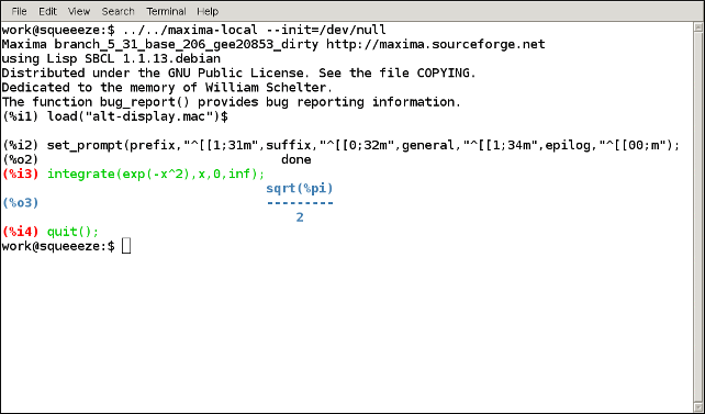
Each prompt string starts with the ASCII escape character (27) followed by an open square bracket (91); each string ends with a lower-case m (109). The webpages https://misc.flogisoft.com/bash/tip_colors_and_formatting and https://www.tldp.org/HOWTO/Bash-Prompt-HOWTO/x329.html provide information on how to use control strings to set the terminal colors.
Categories: Package alt-display ·
Next: Package atensor, Previous: Package alt-display [Contents][Index]
38 Package asympa
Next: Functions and variables for asympa, Previous: Package asympa, Up: Package asympa [Contents][Index]
38.1 Introduction to asympa
- Function: asympa 
asympais a package for asymptotic analysis. The package contains simplification functions for asymptotic analysis, including the “big O” and “little o” functions that are widely used in complexity analysis and numerical analysis.load ("asympa")loads this package.Categories: Package asympa ·
Previous: Introduction to asympa, Up: Package asympa [Contents][Index]
38.2 Functions and variables for asympa
Next: Package augmented_lagrangian, Previous: Package asympa [Contents][Index]
39 Package atensor
Next: Functions and Variables for atensor, Previous: Package atensor, Up: Package atensor [Contents][Index]
39.1 Introduction to atensor
atensor is an algebraic tensor manipulation package. To use atensor,
type load("atensor"), followed by a call to the init_atensor
function.
For alternative packages for handling tensors see Package ctensor and Package itensor.
The essence of atensor is a set of simplification rules for the
noncommutative (dot) product operator ("."). atensor recognizes
several algebra types; the corresponding simplification rules are put
into effect when the init_atensor function is called.
The capabilities of atensor can be demonstrated by defining the
algebra of quaternions as a Clifford-algebra Cl(0,2) with two basis
vectors. The three quaternionic imaginary units are then the two
basis vectors and their product, i.e.:
i = v j = v k = v . v
1 2 1 2
Although the atensor package has a built-in definition for the
quaternion algebra, it is not used in this example, in which we
endeavour to build the quaternion multiplication table as a matrix:
(%i1) load("atensor");
(%o1) /share/tensor/atensor.mac
(%i2) init_atensor(clifford,0,0,2);
(%o2) done
(%i3) atensimp(v[1].v[1]);
(%o3) - 1
(%i4) atensimp((v[1].v[2]).(v[1].v[2]));
(%o4) - 1
(%i5) q:zeromatrix(4,4);
[ 0 0 0 0 ]
[ ]
[ 0 0 0 0 ]
(%o5) [ ]
[ 0 0 0 0 ]
[ ]
[ 0 0 0 0 ]
(%i6) q[1,1]:1;
(%o6) 1
(%i7) for i thru adim do q[1,i+1]:q[i+1,1]:v[i];
(%o7) done
(%i8) q[1,4]:q[4,1]:v[1].v[2];
(%o8) v . v
1 2
(%i9) for i from 2 thru 4 do for j from 2 thru 4 do
q[i,j]:atensimp(q[i,1].q[1,j]);
(%o9) done
(%i10) q;
[ 1 v v v . v ]
[ 1 2 1 2 ]
[ ]
[ v - 1 v . v - v ]
[ 1 1 2 2 ]
(%o10) [ ]
[ v - v . v - 1 v ]
[ 2 1 2 1 ]
[ ]
[ v . v v - v - 1 ]
[ 1 2 2 1 ]
atensor recognizes as base vectors indexed symbols, where the symbol
is that stored in asymbol and the index runs between 1 and adim.
For indexed symbols, and indexed symbols only, the bilinear forms
sf, af, and av are evaluated. The evaluation
substitutes the value of aform[i,j] in place of fun(v[i],v[j])
where v represents the value of asymbol and fun is
either af or sf; or, it substitutes v[aform[i,j]]
in place of av(v[i],v[j]).
Needless to say, the functions sf, af and av
can be redefined.
When the atensor package is loaded, the following flags are set:
dotscrules:true; dotdistrib:true; dotexptsimp:false;
If you wish to experiment with a nonassociative algebra, you may also
consider setting dotassoc to false. In this case, however,
atensimp will not always be able to obtain the desired
simplifications.
Previous: Introduction to atensor, Up: Package atensor [Contents][Index]
39.2 Functions and Variables for atensor
- Function: init_atensor
init_atensor (alg_type, opt_dims)
init_atensor (alg_type) ¶ -
Initializes the
atensorpackage with the specified algebra type. alg_type can be one of the following:universal: The universal algebra has no commutation rules.grassmann: The Grassman algebra is defined by the commutation relationu.v+v.u=0.clifford: The Clifford algebra is defined by the commutation relationu.v+v.u=-2*sf(u,v)wheresfis a symmetric scalar-valued function. For this algebra, opt_dims can be up to three nonnegative integers, representing the number of positive, degenerate, and negative dimensions of the algebra, respectively. If any opt_dims values are supplied,atensorwill configure the values ofadimandaformappropriately. Otherwise,adimwill default to 0 andaformwill not be defined.symmetric: The symmetric algebra is defined by the commutation relationu.v-v.u=0.symplectic: The symplectic algebra is defined by the commutation relationu.v-v.u=2*af(u,v)whereafis an antisymmetric scalar-valued function. For the symplectic algebra, opt_dims can be up to two nonnegative integers, representing the nondegenerate and degenerate dimensions, respectively. If any opt_dims values are supplied,atensorwill configure the values ofadimandaformappropriately. Otherwise,adimwill default to 0 andaformwill not be defined.lie_envelop: The algebra of the Lie envelope is defined by the commutation relationu.v-v.u=2*av(u,v)whereavis an antisymmetric function.The
init_atensorfunction also recognizes several predefined algebra types:compleximplements the algebra of complex numbers as the Clifford algebra Cl(0,1). The callinit_atensor(complex)is equivalent toinit_atensor(clifford,0,0,1).quaternionimplements the algebra of quaternions. The callinit_atensor (quaternion)is equivalent toinit_atensor (clifford,0,0,2).pauliimplements the algebra of Pauli-spinors as the Clifford-algebra Cl(3,0). A call toinit_atensor(pauli)is equivalent toinit_atensor(clifford,3).diracimplements the algebra of Dirac-spinors as the Clifford-algebra Cl(3,1). A call toinit_atensor(dirac)is equivalent toinit_atensor(clifford,3,0,1).Categories: Package atensor ·
- Function: atensimp (expr) 
-
Simplifies an algebraic tensor expression expr according to the rules configured by a call to
init_atensor. Simplification includes recursive application of commutation relations and resolving calls tosf,af, andavwhere applicable. A safeguard is used to ensure that the function always terminates, even for complex expressions.Categories: Package atensor · Simplification functions ·
- Function: alg_type 
The algebra type. Valid values are
universal,grassmann,clifford,symmetric,symplecticandlie_envelop.Categories: Package atensor ·
- Variable: adim 
Default value: 0
The dimensionality of the algebra.
atensoruses the value ofadimto determine if an indexed object is a valid base vector. Seeabasep.Categories: Package atensor · Global variables ·
- Variable: aform 
Default value:
ident(3)Default values for the bilinear forms
sf,af, andav. The default is the identity matrixident(3).Categories: Package atensor · Global variables ·
- Variable: asymbol 
Default value:
vThe symbol for base vectors.
Categories: Package atensor · Global variables ·
- Function: sf (u, v) 
-
A symmetric scalar function that is used in commutation relations. The default implementation checks if both arguments are base vectors using
abasepand if that is the case, substitutes the corresponding value from the matrixaform.Categories: Package atensor ·
- Function: af (u, v) 
-
An antisymmetric scalar function that is used in commutation relations. The default implementation checks if both arguments are base vectors using
abasepand if that is the case, substitutes the corresponding value from the matrixaform.Categories: Package atensor ·
- Function: av (u, v) 
-
An antisymmetric function that is used in commutation relations. The default implementation checks if both arguments are base vectors using
abasepand if that is the case, substitutes the corresponding value from the matrixaform.For instance:
(%i1) load("atensor"); (%o1) /share/tensor/atensor.mac (%i2) adim:3; (%o2) 3 (%i3) aform:matrix([0,3,-2],[-3,0,1],[2,-1,0]); [ 0 3 - 2 ] [ ] (%o3) [ - 3 0 1 ] [ ] [ 2 - 1 0 ] (%i4) asymbol:x; (%o4) x (%i5) av(x[1],x[2]); (%o5) x 3Categories: Package atensor ·
- Function: abasep (v) 
-
Checks if its argument is an
atensorbase vector. That is, if it is an indexed symbol, with the symbol being the same as the value ofasymbol, and the index having a numeric value between 1 andadim.Categories: Package atensor · Predicate functions ·
Next: Package bernstein, Previous: Package atensor [Contents][Index]
40 Package augmented_lagrangian
Previous: Package augmented_lagrangian, Up: Package augmented_lagrangian [Contents][Index]
40.1 Functions and Variables for augmented_lagrangian
- Function: augmented_lagrangian_method
augmented_lagrangian_method (FOM, xx, C, yy)
augmented_lagrangian_method (FOM, xx, C, yy, optional_args)
augmented_lagrangian_method ([FOM, grad], xx, C, yy)
augmented_lagrangian_method ([FOM, grad], xx, C, yy, optional_args) ¶ -
Returns an approximate minimum of the expression FOM with respect to the variables xx, holding the constraints C equal to zero. yy is a list of initial guesses for xx. The method employed is the augmented Lagrangian method (see Refs [1] and [2]).
grad, if present, is the gradient of FOM with respect to xx, represented as a list of expressions, one for each variable in xx. If not present, the gradient is constructed automatically.
FOM and each element of grad, if present, must be ordinary expressions, not names of functions or lambda expressions.
optional_argsrepresents additional arguments, specified assymbol = value. The optional arguments recognized are:niterNumber of iterations of the augmented Lagrangian algorithm
lbfgs_toleranceTolerance supplied to LBFGS
iprintIPRINT parameter (a list of two integers which controls verbosity) supplied to LBFGS
%lambdaInitial value of
%lambdato be used for calculating the augmented Lagrangian
This implementation minimizes the augmented Lagrangian by applying the limited-memory BFGS (LBFGS) algorithm, which is a quasi-Newton algorithm.
load("augmented_lagrangian")loads this function.See also Package lbfgs
References:
[1] http://www-fp.mcs.anl.gov/otc/Guide/OptWeb/continuous/constrained/nonlinearcon/auglag.html
[2] http://www.cs.ubc.ca/spider/ascher/542/chap10.pdf
Examples:
(%i1) load ("lbfgs"); (%o1) /home/gunter/src/maxima-code/share/lbfgs/lbfgs.mac(%i2) load ("augmented_lagrangian"); (%o2) /home/gunter/src/maxima-code/share/contrib/augmented_lagra\ ngian.mac(%i3) FOM: x^2 + 2*y^2; 2 2 (%o3) 2 y + x(%i4) xx: [x, y]; (%o4) [x, y]
(%i5) C: [x + y - 1]; (%o5) [y + x - 1]
(%i6) yy: [1, 1]; (%o6) [1, 1]
(%i7) augmented_lagrangian_method(FOM, xx, C, yy, iprint=[-1,0]); (%o7) [[x = 0.666659841080023, y = 0.333340272455448], %lambda = [- 1.333337940892518]]Same example as before, but this time the gradient is supplied as an argument.
(%i1) load ("lbfgs")$ (%i2) load ("augmented_lagrangian")$(%i3) FOM: x^2 + 2*y^2; 2 2 (%o3) 2 y + x(%i4) xx: [x, y]; (%o4) [x, y]
(%i5) grad : [2*x, 4*y]; (%o5) [2 x, 4 y]
(%i6) C: [x + y - 1]; (%o6) [y + x - 1]
(%i7) yy: [1, 1]; (%o7) [1, 1]
(%i8) augmented_lagrangian_method ([FOM, grad], xx, C, yy, iprint = [-1, 0]); (%o8) [[x = 0.6666598410800247, y = 0.3333402724554464], %lambda = [- 1.333337940892525]]
Next: Package bitwise, Previous: Package augmented_lagrangian [Contents][Index]
41 Package bernstein
Previous: Package bernstein, Up: Package bernstein [Contents][Index]
41.1 Functions and Variables for Bernstein
- Function: bernstein_poly (k, n, x) 
-
Provided
kis not a negative integer, the Bernstein polynomials are defined bybernstein_poly(k,n,x) = binomial(n,k) x^k (1-x)^(n-k); for a negative integerk, the Bernstein polynomialbernstein_poly(k,n,x)vanishes. When eitherkornare non integers, the option variablebernstein_explicitcontrols the expansion of the Bernstein polynomials into its explicit form; example:(%i1) load("bernstein")$ (%i2) bernstein_poly(k,n,x); (%o2) bernstein_poly(k, n, x) (%i3) bernstein_poly(k,n,x), bernstein_explicit : true; n - k k (%o3) binomial(n, k) (1 - x) xThe Bernstein polynomials have both a gradef property and an integrate property:
(%i4) diff(bernstein_poly(k,n,x),x); (%o4) (bernstein_poly(k - 1, n - 1, x) - bernstein_poly(k, n - 1, x)) n (%i5) integrate(bernstein_poly(k,n,x),x); (%o5) k + 1 hypergeometric([k + 1, k - n], [k + 2], x) binomial(n, k) x ---------------------------------------------------------------- k + 1For numeric inputs, both real and complex, the Bernstein polynomials evaluate to a numeric result:
(%i6) bernstein_poly(5,9, 1/2 + %i); 39375 %i 39375 (%o6) -------- + ----- 128 256 (%i7) bernstein_poly(5,9, 0.5b0 + %i); (%o7) 3.076171875b2 %i + 1.5380859375b2To use
bernstein_poly, firstload("bernstein").
- Variable: bernstein_explicit 
Default value:
falseWhen either
kornare non integers, the option variablebernstein_explicitcontrols the expansion ofbernstein(k,n,x)into its explicit form; example:(%i1) bernstein_poly(k,n,x); (%o1) bernstein_poly(k, n, x) (%i2) bernstein_poly(k,n,x), bernstein_explicit : true; n - k k (%o2) binomial(n, k) (1 - x) xWhen both
kandnare explicitly integers,bernstein(k,n,x)always expands to its explicit form.
- Function: multibernstein_poly ([k1,k2,…, kp], [n1,n2,…, np], [x1,x2,…, xp]) 
-
The multibernstein polynomial
multibernstein_poly ([k1, k2, ..., kp], [n1, n2, ..., np], [x1, x2, ..., xp])is the product of bernstein polynomialsbernstein_poly(k1, n1, x1) bernstein_poly(k2, n2, x2) ... bernstein_poly(kp, np, xp).To use
multibernstein_poly, firstload("bernstein").
- Function: bernstein_approx (f, [x1, x1, …, xn], n) 
-
Return the
n-th order uniform Bernstein polynomial approximation for the function(x1, x2, ..., xn) |--> f. Examples(%i1) bernstein_approx(f(x),[x], 2); 2 1 2 (%o1) f(1) x + 2 f(-) (1 - x) x + f(0) (1 - x) 2 (%i2) bernstein_approx(f(x,y),[x,y], 2); 2 2 1 2 (%o2) f(1, 1) x y + 2 f(-, 1) (1 - x) x y 2 2 2 1 2 + f(0, 1) (1 - x) y + 2 f(1, -) x (1 - y) y 2 1 1 1 2 + 4 f(-, -) (1 - x) x (1 - y) y + 2 f(0, -) (1 - x) (1 - y) y 2 2 2 2 2 1 2 + f(1, 0) x (1 - y) + 2 f(-, 0) (1 - x) x (1 - y) 2 2 2 + f(0, 0) (1 - x) (1 - y)To use
bernstein_approx, firstload("bernstein").
- Function: bernstein_expand (e, [x1, x1, …, xn]) 
-
Express the polynomial
eexactly as a linear combination of multi-variable Bernstein polynomials.(%i1) bernstein_expand(x*y+1,[x,y]); (%o1) 2 x y + (1 - x) y + x (1 - y) + (1 - x) (1 - y) (%i2) expand(%); (%o2) x y + 1
Maxima signals an error when the first argument isn’t a polynomial.
To use
bernstein_expand, firstload("bernstein").
Next: Package bode, Previous: Package bernstein [Contents][Index]
42 Package bitwise
The package bitwise provides functions that allow to manipulate
bits of integer constants. As always maxima attempts to simplify the result
of the operation if the actual value of a constant isn’t known considering
attributes that might be known for the variables, see the declare
mechanism.
42.1 Functions and Variables for bitwise
- Function: bit_not (int) 
-
Inverts all bits of a signed integer. The result of this action reads
-int - 1.(%i1) load("bitwise")$(%i2) bit_not(i); (%o2) bit_not(i)
(%i3) bit_not(bit_not(i)); (%o3) i
(%i4) bit_not(3); (%o4) - 4
(%i5) bit_not(100); (%o5) - 101
(%i6) bit_not(-101); (%o6) 100
- Function: bit_and (int1, ...) 
-
This function calculates a bitwise
andof two or more signed integers.(%i1) load("bitwise")$(%i2) bit_and(i,i); (%o2) i
(%i3) bit_and(i,i,i); (%o3) i
(%i4) bit_and(1,3); (%o4) 1
(%i5) bit_and(-7,7); (%o5) 1
If it is known if one of the parameters to
bit_andis even this information is taken into consideration by the function.(%i1) load("bitwise")$(%i2) declare(e,even,o,odd); (%o2) done
(%i3) bit_and(1,e); (%o3) 0
(%i4) bit_and(1,o); (%o4) 1
- Function: bit_or (int1, ...) 
-
This function calculates a bitwise
orof two or more signed integers.(%i1) load("bitwise")$(%i2) bit_or(i,i); (%o2) i
(%i3) bit_or(i,i,i); (%o3) i
(%i4) bit_or(1,3); (%o4) 3
(%i5) bit_or(-7,7); (%o5) - 1
If it is known if one of the parameters to
bit_oris even this information is taken into consideration by the function.(%i1) load("bitwise")$(%i2) declare(e,even,o,odd); (%o2) done
(%i3) bit_or(1,e); (%o3) e + 1
(%i4) bit_or(1,o); (%o4) o
- Function: bit_xor (int1, ...) 
-
This function calculates a bitwise
orof two or more signed integers.(%i1) load("bitwise")$(%i2) bit_xor(i,i); (%o2) 0
(%i3) bit_xor(i,i,i); (%o3) i
(%i4) bit_xor(1,3); (%o4) 2
(%i5) bit_xor(-7,7); (%o5) - 2
If it is known if one of the parameters to
bit_xoris even this information is taken into consideration by the function.(%i1) load("bitwise")$(%i2) declare(e,even,o,odd); (%o2) done
(%i3) bit_xor(1,e); (%o3) e + 1
(%i4) bit_xor(1,o); (%o4) o - 1
- Function: bit_lsh (int, nBits) 
-
This function shifts all bits of the signed integer
intto the left bynBitsbits. The width of the integer is extended bynBitsfor this process. The result ofbit_lshtherefore isint * 2.(%i1) load("bitwise")$(%i2) bit_lsh(0,1); (%o2) 0
(%i3) bit_lsh(1,0); (%o3) 1
(%i4) bit_lsh(1,1); (%o4) 2
(%i5) bit_lsh(1,i); (%o5) bit_lsh(1, i)
(%i6) bit_lsh(-3,1); (%o6) - 6
(%i7) bit_lsh(-2,1); (%o7) - 4
- Function: bit_rsh (int, nBits) 
-
This function shifts all bits of the signed integer
intto the right bynBitsbits. The width of the integer is reduced bynBitsfor this process.(%i1) load("bitwise")$(%i2) bit_rsh(0,1); (%o2) 0
(%i3) bit_rsh(2,0); (%o3) 2
(%i4) bit_rsh(2,1); (%o4) 1
(%i5) bit_rsh(2,2); (%o5) 0
(%i6) bit_rsh(-3,1); (%o6) - 2
(%i7) bit_rsh(-2,1); (%o7) - 1
(%i8) bit_rsh(-2,2); (%o8) - 1
- Function: bit_length (int) 
-
determines how many bits a variable needs to be long in order to store the number
int. This function only operates on positive numbers.(%i1) load("bitwise")$(%i2) bit_length(0); (%o2) 0
(%i3) bit_length(1); (%o3) 1
(%i4) bit_length(7); (%o4) 3
(%i5) bit_length(8); (%o5) 4
- Function: bit_onep (int, nBit) 
-
determines if bits
nBitis set in the signed integerint.(%i1) load("bitwise")$(%i2) bit_onep(85,0); (%o2) true
(%i3) bit_onep(85,1); (%o3) false
(%i4) bit_onep(85,2); (%o4) true
(%i5) bit_onep(85,3); (%o5) false
(%i6) bit_onep(85,100); (%o6) false
(%i7) bit_onep(i,100); (%o7) bit_onep(i, 100)
For signed numbers the sign bit is interpreted to be more than
nBitto the left of the leftmost bit ofintthat reads1.(%i1) load("bitwise")$(%i2) bit_onep(-2,0); (%o2) false
(%i3) bit_onep(-2,1); (%o3) true
(%i4) bit_onep(-2,2); (%o4) true
(%i5) bit_onep(-2,3); (%o5) true
(%i6) bit_onep(-2,4); (%o6) true
If it is known if the number to be tested is even this information is taken into consideration by the function.
(%i1) load("bitwise")$(%i2) declare(e,even,o,odd); (%o2) done
(%i3) bit_onep(e,0); (%o3) false
(%i4) bit_onep(o,0); (%o4) true
Next: Package cartan, Previous: Package bitwise [Contents][Index]
43 Package bode
Previous: Package bode, Up: Package bode [Contents][Index]
43.1 Functions and Variables for bode
- Function: bode_gain (H, range, ...plot_opts...) 
Function to draw Bode gain plots.
Examples (1 through 7 from
8 from Ron Crummett):
(%i1) load("bode")$ (%i2) H1 (s) := 100 * (1 + s) / ((s + 10) * (s + 100))$ (%i3) bode_gain (H1 (s), [w, 1/1000, 1000])$ (%i4) H2 (s) := 1 / (1 + s/omega0)$ (%i5) bode_gain (H2 (s), [w, 1/1000, 1000]), omega0 = 10$ (%i6) H3 (s) := 1 / (1 + s/omega0)^2$ (%i7) bode_gain (H3 (s), [w, 1/1000, 1000]), omega0 = 10$ (%i8) H4 (s) := 1 + s/omega0$ (%i9) bode_gain (H4 (s), [w, 1/1000, 1000]), omega0 = 10$ (%i10) H5 (s) := 1/s$ (%i11) bode_gain (H5 (s), [w, 1/1000, 1000])$ (%i12) H6 (s) := 1/((s/omega0)^2 + 2 * zeta * (s/omega0) + 1)$ (%i13) bode_gain (H6 (s), [w, 1/1000, 1000]), omega0 = 10, zeta = 1/10$ (%i14) H7 (s) := (s/omega0)^2 + 2 * zeta * (s/omega0) + 1$ (%i15) bode_gain (H7 (s), [w, 1/1000, 1000]), omega0 = 10, zeta = 1/10$ (%i16) H8 (s) := 0.5 / (0.0001 * s^3 + 0.002 * s^2 + 0.01 * s)$ (%i17) bode_gain (H8 (s), [w, 1/1000, 1000])$To use this function write first
load("bode"). See alsobode_phase.Categories: Plotting · Package bode ·
- Function: bode_phase (H, range, ...plot_opts...) 
Function to draw Bode phase plots.
Examples (1 through 7 from
8 from Ron Crummett):
(%i1) load("bode")$ (%i2) H1 (s) := 100 * (1 + s) / ((s + 10) * (s + 100))$ (%i3) bode_phase (H1 (s), [w, 1/1000, 1000])$ (%i4) H2 (s) := 1 / (1 + s/omega0)$ (%i5) bode_phase (H2 (s), [w, 1/1000, 1000]), omega0 = 10$ (%i6) H3 (s) := 1 / (1 + s/omega0)^2$ (%i7) bode_phase (H3 (s), [w, 1/1000, 1000]), omega0 = 10$ (%i8) H4 (s) := 1 + s/omega0$ (%i9) bode_phase (H4 (s), [w, 1/1000, 1000]), omega0 = 10$ (%i10) H5 (s) := 1/s$ (%i11) bode_phase (H5 (s), [w, 1/1000, 1000])$ (%i12) H6 (s) := 1/((s/omega0)^2 + 2 * zeta * (s/omega0) + 1)$ (%i13) bode_phase (H6 (s), [w, 1/1000, 1000]), omega0 = 10, zeta = 1/10$ (%i14) H7 (s) := (s/omega0)^2 + 2 * zeta * (s/omega0) + 1$ (%i15) bode_phase (H7 (s), [w, 1/1000, 1000]), omega0 = 10, zeta = 1/10$ (%i16) H8 (s) := 0.5 / (0.0001 * s^3 + 0.002 * s^2 + 0.01 * s)$ (%i17) bode_phase (H8 (s), [w, 1/1000, 1000])$ (%i18) block ([bode_phase_unwrap : false], bode_phase (H8 (s), [w, 1/1000, 1000])); (%i19) block ([bode_phase_unwrap : true], bode_phase (H8 (s), [w, 1/1000, 1000]));To use this function write first
load("bode"). See alsobode_gain.Categories: Plotting · Package bode ·
Next: Package celine, Previous: Package bode [Contents][Index]
44 Package cartan
Next: Functions and Variables for cartan, Previous: Package cartan, Up: Package cartan [Contents][Index]
44.1 Introduction to cartan
cartan is a package which implements the calculus of differential
forms. Included are facilities for computing exterior products,
contraction of vectors and forms, exterior derivatives, and Lie
derivatives. The differential forms are given in terms of the natural
basis forms derived from the coordinates on the manifold. Type
load(cartan); to load this package. For a demonstration, type
demo(cartan);
cartan was implemented by F.B. Estabrook and H.D. Wahlquist.
Previous: Introduction to cartan, Up: Package cartan [Contents][Index]
44.2 Functions and Variables for cartan
- Function: init_cartan ([x_1, …, x_m]) 
Initializes some global variables for the package. The argument, a Maxima list, is an ordered list of coordinates. The coordinate list is stored as the value of the variable
cartan_coords. The value of the variablecartan_basisis a list of the basis 1-forms. The dimension is stored as the value of the variablecartan_dim.
(%i1) load("cartan")$
(%i2) init_cartan([x,y,z]);
(%o2) [dx, dy, dz]
(%i3) cartan_basis;
(%o3) [dx, dy, dz]
(%i4) cartan_dim;
(%o4) 3
- Infix Operator: ~ 
The tilde “~” is an infix operator which denotes the exterior (wedge) product. The canonical ordering of the products is determined by the order in which the coordinates were specified. For example, if the coordinate list is specified as
[x,y,z], then the two-formdy~dxsimplifies to-dx~dy.
(%i1) init_cartan([x,y,z]); (%o1) [dx, dy, dz] (%i2) vr:[v1,v2,v3]; (%o2) [v1, v2, v3] (%i3) f1:x~dy+z~dz; (%o3) z dz + x dy (%i4) f2:dz~f1; (%o4) - x dy dz
- Infix Operator: | 
The bar “|” is an infix operator which defines the contraction of a vector on a form. The vector should be given on the left.
- Function: ext_diff (form) 
The exterior derivative operator. It takes one argument, which should be a differential form.
- Function: lie_diff (vector1,[vector2,form]) 
The Lie derivative operator. The first argument is a vector field. The second argument may be either a vector field or a differential form.
(Note: display2d is set to false in the following example.)
(%i1) init_cartan([x,y,z]);
(%o1) [dx,dy,dz]
(%i2) vr:[v1,v2,v3];
(%o2) [v1,v2,v3]
(%i3) f1:x ~ dy+z ~ dz;
(%o3) z*dz+x*dy
(%i4) vr | f1;
(%o4) v3*z+v2*x
(%i5) f2:dz ~ f1;
(%o5) -(x*dy*dz)
(%i6) ext_diff(f1);
(%o6) dx*dy
(%i7) ext_diff(f3(x,y,z) ~ dx);
(%o7) -('diff(f3(x,y,z),z,1)*dx*dz)-'diff(f3(x,y,z),y,1)*dx*dy
(%i8) depends([v1,v2,v3],[x,y,z]);
(%o8) [v1(x,y,z),v2(x,y,z),v3(x,y,z)]
(%i9) lie_diff(vr,f2);
(%o9) -('diff(v3,z,1)*x*dy*dz)-'diff(v2,y,1)*x*dy*dz-v1*dy*dz
-'diff(v2,x,1)*x*dx*dz+'diff(v3,x,1)*x*dx*dy
(%i10) depends([w1,w2,w3],[x,y,z]);
(%o10) [w1(x,y,z),w2(x,y,z),w3(x,y,z)]
(%i11) wr:[w1,w2,w3];
(%o11) [w1,w2,w3]
(%i12) lie_diff(vr,wr);
(%o12) [-('diff(v1,z,1)*w3)-'diff(v1,y,1)*w2+v3*'diff(w1,z,1)+v2*'diff(w1,y,1)
+v1*'diff(w1,x,1)-'diff(v1,x,1)*w1,
-('diff(v2,z,1)*w3)+v3*'diff(w2,z,1)+v2*'diff(w2,y,1)+v1*'diff(w2,x,1)
-'diff(v2,y,1)*w2-'diff(v2,x,1)*w1,
v3*'diff(w3,z,1)+v2*'diff(w3,y,1)+v1*'diff(w3,x,1)-'diff(v3,z,1)*w3
-'diff(v3,y,1)*w2-'diff(v3,x,1)*w1]
Next: Package clebsch_gordan, Previous: Package cartan [Contents][Index]
45 Package celine
Up: Package celine [Contents][Index]
45.1 Introduction to celine
Maxima implementation of Sister Celine’s method. Barton Willis wrote this code. It is released under the Creative Commons CC0 license.
Celine’s method is described in Sections 4.1–4.4 of the book "A=B", by Marko Petkovsek, Herbert S. Wilf, and Doron Zeilberger. This book is available at http://www.math.rutgers.edu/~zeilberg/AeqB.pdf
Let f = F(n,k). The function celine returns a set of recursion relations for F of the form
p_0(n) * fff(n,k) + p_1(n) * fff(n+1,k) + ... + p_p(n) * fff(n+p,k+q),
where p_0 through p_p are polynomials. If Maxima is unable to determine that sum(sum(a(i,j) * F(n+i,k+j),i,0,p),j,0,q) / F(n,k) is a rational function of n and k, celine returns the empty set. When f involves parameters (variables other than n or k), celine might make assumptions about these parameters. Using ’put’ with a key of ’proviso,’ Maxima saves these assumptions on the input label.
To use this function, first load the package integer_sequence, opsubst, and to_poly_solve.
Examples:
(%i1) load("integer_sequence")$
(%i2) load("opsubst")$
(%i3) load("to_poly_solve")$
(%i4) load("celine")$
(%i5) celine(n!,n,k,1,0);
(%o5) {fff(n + 1, k) - n fff(n, k) - fff(n, k)}
Verification that this result is correct:
(%i1) load("integer_sequence")$
(%i2) load("opsubst")$
(%i3) load("to_poly_solve")$
(%i4) load("celine")$
(%i5) g1:{fff(n+1,k)-n*fff(n,k)-fff(n,k)};
(%o5) {fff(n + 1, k) - n fff(n, k) - fff(n, k)}
(%i6) ratsimp(minfactorial(first(g1))),fff(n,k) := n!; (%o6) 0
An example with parameters including the test that the result of the example is correct:
(%i1) load("integer_sequence")$
(%i2) load("opsubst")$
(%i3) load("to_poly_solve")$
(%i4) load("celine")$
(%i5) e : pochhammer(a,k) * pochhammer(-k,n) / (pochhammer(b,k));
(a) (- k)
k n
(%o5) -----------
(b)
k
(%i6) recur : celine(e,n,k,2,1);
(%o6) {fff(n + 2, k + 1) - fff(n + 2, k) - b fff(n + 1, k + 1)
+ n ((- fff(n + 1, k + 1)) + 2 fff(n + 1, k) - a fff(n, k)
- fff(n, k)) + a (fff(n + 1, k) - fff(n, k)) + 2 fff(n + 1, k)
2
- n fff(n, k)}
(%i7) /* Test this result for correctness */ (%i8) first(%), fff(n,k) := ''(e)$
(%i9) makefact(makegamma(%))$ (%o9) 0
(%i10) minfactorial(factor(minfactorial(factor(%))));
The proviso data suggests that setting a = b may result in a lower order recursion which is shown by the following example:
(%i1) load("integer_sequence")$
(%i2) load("opsubst")$
(%i3) load("to_poly_solve")$
(%i4) load("celine")$
(%i5) e : pochhammer(a,k) * pochhammer(-k,n) / (pochhammer(b,k));
(a) (- k)
k n
(%o5) -----------
(b)
k
(%i6) recur : celine(e,n,k,2,1);
(%o6) {fff(n + 2, k + 1) - fff(n + 2, k) - b fff(n + 1, k + 1)
+ n ((- fff(n + 1, k + 1)) + 2 fff(n + 1, k) - a fff(n, k)
- fff(n, k)) + a (fff(n + 1, k) - fff(n, k)) + 2 fff(n + 1, k)
2
- n fff(n, k)}
(%i7) get('%,'proviso);
(%o7) false
(%i8) celine(subst(b=a,e),n,k,1,1);
(%o8) {fff(n + 1, k + 1) - fff(n + 1, k) + n fff(n, k)
+ fff(n, k)}
Next: Package cobyla, Previous: Package celine [Contents][Index]
46 Package clebsch_gordan
Previous: Package clebsch_gordan, Up: Package clebsch_gordan [Contents][Index]
46.1 Functions and Variables for clebsch_gordan
- Function: clebsch_gordan (j1, j2, m1, m2, j, m) 
-
Compute the Clebsch-Gordan coefficient <j1, j2, m1, m2 | j, m>.
Categories: clebsch_gordan ·
- Function: racah_v (a, b, c, a1, b1, c1) 
-
Compute Racah’s V coefficient (computed in terms of a related Clebsch-Gordan coefficient).
Categories: clebsch_gordan ·
- Function: racah_w (j1, j2, j5, j4, j3, j6) 
-
Compute Racah’s W coefficient (computed in terms of a Wigner 6j symbol)
Categories: clebsch_gordan ·
- Function: wigner_3j (j1, j2, j3, m1, m2, m3) 
-
Compute Wigner’s 3j symbol (computed in terms of a related Clebsch-Gordan coefficient).
Categories: clebsch_gordan ·
- Function: wigner_6j (j1, j2, j3, j4, j5, j6) 
-
Compute Wigner’s 6j symbol.
Categories: clebsch_gordan ·
- Function: wigner_9j (a, b, c, d, e, f, g, h, i, j,) 
-
Compute Wigner’s 9j symbol.
Categories: clebsch_gordan ·
Next: Package colnew, Previous: Package clebsch_gordan [Contents][Index]
47 Package cobyla
Next: Functions and Variables for cobyla, Previous: Package cobyla, Up: Package cobyla [Contents][Index]
47.1 Introduction to cobyla
fmin_cobyla is a Common Lisp translation (via f2cl) of the
Fortran constrained optimization routine COBYLA by Powell[1][2][3].
COBYLA minimizes an objective function F(X) subject to M inequality constraints of the form \(g(X) \ge 0\) on X, where X is a vector of variables that has N components.
Equality constraints g(X) = 0 can often be implemented by a pair of inequality constraints \(g(X) \ge 0\) and \(-g(X) \ge 0.\) Maxima’s interface to COBYLA allows equality constraints and internally converts the equality constraints to a pair of inequality constraints.
The algorithm employs linear approximations to the objective and constraint functions, the approximations being formed by linear interpolation at N+1 points in the space of the variables. The interpolation points are regarded as vertices of a simplex. The parameter RHO controls the size of the simplex and it is reduced automatically from RHOBEG to RHOEND. For each RHO the subroutine tries to achieve a good vector of variables for the current size, and then RHO is reduced until the value RHOEND is reached. Therefore, RHOBEG and RHOEND should be set to reasonable initial changes to and the required accuracy in the variables respectively, but this accuracy should be viewed as a subject for experimentation because it is not guaranteed. The routine treats each constraint individually when calculating a change to the variables, rather than lumping the constraints together into a single penalty function. The name of the subroutine is derived from the phrase Constrained Optimization BY Linear Approximations.
References:
[1] Fortran Code is from http://plato.asu.edu/sub/nlores.html#general
[2] M. J. D. Powell, "A direct search optimization method that models the objective and constraint functions by linear interpolation," in Advances in Optimization and Numerical Analysis, eds. S. Gomez and J.-P. Hennart (Kluwer Academic: Dordrecht, 1994), p. 51-67. doi:10.1007/978-94-015-8330-5_4
[3] M. J. D. Powell, "Direct search algorithms for optimization calculations," Acta Numerica 7, 287-336 (1998). doi:10.1017/S0962492900002841 Also available as University of Cambridge, Department of Applied Mathematics and Theoretical Physics, Numerical Analysis Group, Report NA1998/04 from https://web.archive.org/web/20160607190705/http://www.damtp.cam.ac.uk:80/user/na/reports.html
Next: Examples for cobyla, Previous: Introduction to cobyla, Up: Package cobyla [Contents][Index]
47.2 Functions and Variables for cobyla
- Function: fmin_cobyla
fmin_cobyla (F, X, Y)
fmin_cobyla (F, X, Y, optional_args) ¶ -
Returns an approximate minimum of the expression F with respect to the variables X, subject to an optional set of constraints. Y is a list of initial guesses for X.
F must be ordinary expressions, not names of functions or lambda expressions.
optional_argsrepresents additional arguments, specified assymbol = value. The optional arguments recognized are:constraintsList of inequality and equality constraints that must be satisfied by X. The inequality constraints must be actual inequalities of the form \(g(X) \ge h(X)\) or \(g(X) \le h(X).\) The equality constraints must be of the form \(g(X) = h(X).\)
rhobegInitial value of the internal RHO variable which controls the size of simplex. (Defaults to 1.0)
rhoendThe desired final value rho parameter. It is approximately the accuracy in the variables. (Defaults to 1d-6.)
iprintVerbose output level. (Defaults to 0)
- 0 - No output
- 1 - Summary at the end of the calculation
- 2 - Each new value of RHO and SIGMA is printed, including the vector of variables, some function information when RHO is reduced.
- 3 - Like 2, but information is printed when F(X) is computed.
maxfunThe maximum number of function evaluations. (Defaults to 1000).
On return, a vector is given:
- The value of the variables giving the minimum. This is a list of
elements of the form
var = valuefor each of the variables listed in X. - The minimized function value
- The number of function evaluations.
- Return code with the following meanings
- 0 - No errors.
- 1 - Limit on maximum number of function evaluations reached.
- 2 - Rounding errors inhibiting progress.
- -1 - MAXCV value exceeds RHOEND. This indicates that the constraints were probably not satisfied. User should investigate the value of the constraints.
MAXCV stands for “MAXimum Constraint Violation” and is the value of max(0.0, -c1(x), -c2(x),...-cm(x)) where ck(x) denotes the k’th constraint function. (Note that maxima allows constraints of the form f(x) = g(x), which are internally converted to f(x)-g(x) >= 0 and g(x)-f(x) >= 0 which is required by COBYLA).
load("fmin_cobyla")loads this function.
- Function: bf_fmin_cobyla
bf_fmin_cobyla (F, X, Y)
bf_fmin_cobyla (F, X, Y, optional_args) ¶ -
This function is identical to
fmin_cobyla, except that bigfloat operations are used, and the default value for rhoend is10^(fpprec/2).See
fmin_cobylafor more information.load("bf_fmin_cobyla")loads this function.
Previous: Functions and Variables for cobyla, Up: Package cobyla [Contents][Index]
47.3 Examples for cobyla
Minimize \(x_1 x_2\) with \(1-x_1^2-x_2^2 \ge 0.\) The theoretical solution is $$ \eqalign{ x_1 &= {1\over \sqrt{2}} \cr x_2 &= -{1\over \sqrt{2}} } $$
(%i1) load("fmin_cobyla")$
(%i2) fmin_cobyla(x1*x2, [x1, x2], [1,1],
constraints = [x1^2+x2^2<=1], iprint=1);
Normal return from subroutine COBYLA
NFVALS = 64 F =-5.000000E-01 MAXCV = 2.000122E-12
X = 7.071076E-01 -7.071060E-01
(%o2) [[x1 = 0.707107555323284, x2 = - 0.7071060070503778],
- 0.4999999999998015, 64, 0]
Here is the same example but the constraint is \(x_1^2+x_2^2 \le -1\) which is impossible over the reals.
(%i1) fmin_cobyla(x1*x2, [x1, x2], [1,1],
constraints = [x1^2+x2^2 <= -1], iprint=1);
Normal return from subroutine COBYLA
NFVALS = 65 F = 3.016417E-13 MAXCV = 1.000000E+00
X =-3.375179E-07 -8.937057E-07
(%o1) [[x1 = - 3.375178983064622e-7, x2 = - 8.937056510780022e-7],
3.016416530564557e-13, 65, - 1]
(%i2) subst(%o1[2], [x1^2+x2^2 <= -1]);
(%o2) [- 6.847914590915444e-13 <= - 1]
We see the return code (%o1[4]) is -1 indicating that the
constraints may not be satisfied. Substituting the solution into the
constraint equation as shown in %o2 shows that the constraint
is, of course, violated.
There are additional examples in the share/cobyla/ex directory and in share/cobyla/rtest_cobyla.mac.
Next: Package combinatorics, Previous: Package cobyla [Contents][Index]
48 Package colnew
Next: Functions and Variables for colnew, Previous: Package colnew, Up: Package colnew [Contents][Index]
48.1 Introduction to colnew
colnew solves mixed-order systems of boundary-value problems (BVPs) in ordinary differential equations(ODEs). It is a Common Lisp translation (via f2cl) of the Fortran routine COLNEW (see Bader&Ascher 1987).
The method uses collocation at Gaussian points and interpolation using basis functions. Approximate solutions are computed on a sequence of automatically selected meshes until a user-specified set of tolerances is satisfied. A damped Newton’s method is used for the nonlinear iteration.
COLNEW has some advanced features:
- Continuation: Most iterative numerical solvers require an initial guess. There are parameter dependent problems that have an obvious solution for a special value of the parameter (for example a coupling constant vanishes). One can then slowly vary the parameter, solving the problem numerically using as a guess the previous solution, until one gets into a strong coupling regime, hence the name continuation. Sometimes an artificial parameter is introduced to allow the use of continuation.
- Singularities: Another interesting feature of COLNEW is that one can manage singularities in the differential equation by setting interior "boundary points" on the singularities. This is because the differential equation is only imposed in the interior of the intervals, but the solution is checked for continuity and continuity of the derivative on the boundary of the intervals.
- Stiff differential equations: COLNEW can be used for solving some stiff differential equations due to the use of adaptive meshes.
The maxima interface to COLNEW exposes the full power and complexity of the Fortran 77 implementation.
COLNEW is a modification of the package COLSYS (see Ascher 1981a and Ascher 1981b). It incorporates a new basis representation replacing B-splines, and improvements for the linear and nonlinear algebraic equation solvers. The package can be referenced as either COLNEW or COLSYS.
Many practical problems that are not in the standard form accepted by COLNEW can be converted into this form. See Asher&Russell 1981.
Next: Examples for colnew, Previous: Introduction to colnew, Up: Package colnew [Contents][Index]
48.2 Functions and Variables for colnew
- Function: colnew_expert
colnew_expert (ncomp, m, aleft, aright, zeta, ipar, ltol, tol, fixpnt, ispace, fspace, iflag, fsub, dfsub, gsub, dgsub, guess) ¶ -
colnew_expert solves mixed-order systems of boundary-value problems (BVPs) in ordinary differential equations (ODEs) using a numerical collocation method.
colnew_expert returns the list [iflag, fspace, ispace]. iflag is an error flag. Lists fspace and ispace contain the state of the solution and can be: used by
colnew_appslnto calculate solution values at arbitrary points in the solution domain; and passed back to colnew_expert to restart the solution process with different arguments.The function arguments are:
ncompNumber of differential equations (ncomp ≤ 20)
mInteger list of length ncomp. \(m_j\) is the order of the j-th differential equation, with \(1 \le m_j \le 4\) and \(m^* = \sum_j m_j \le 40.\)
aleftLeft end of interval
arightRight end of interval
zetazeta \((\zeta)\) is a real list of length \(m^*.\) \(\zeta_j\) is the j-th boundary or side condition point. The list \(\zeta\) must be ordered, with \(\zeta_j \le \zeta_{j+1}.\) All side condition points must be mesh points in all meshes used, see description of ipar[11] and fixpnt below.
iparA integer list of length 11. The parameters in ipar are:
- ipar[1]
- 0, if the problem is linear
- 1, if the problem is nonlinear
- ipar[2] ( = k )
Number of collocation points per subinterval , where \(\max_j m_j \le k \le 7.\) If ipar[2]=0 then colnew sets \(k = \max\left(\max_i m_i + 5, 5 - \max_i m_i\right).\) - ipar[3] ( = n )
Number of subintervals in the initial mesh.
If ipar[3] = 0 then colnew arbitrarily sets n = 5. - ipar[4] ( = ntol )
Number of solution and derivative tolerances.
Require \(0 < {\rm ntol} < m^*.\) - ipar[5] ( = ndimf )
The length of list fspace. Its size provides a constraint on nmax. Choose ipar[5] according to the formula \({\rm ipar[5]} \ge {\rm nmax} \cdot {\rm nsizef}\) where \({\rm nsizef} = 4 + 3m^* + (5 + {\rm kd})\times{\rm kdm} + (2m^* - {\rm nrec})\times 2 m^*.\) - ipar[6] ( = ndimi )
The length of list ispace. Its size provides a constraint on nmax, the maximum number of subintervals. Choose ipar[6] according to the formula \({\rm ipar[6]} = {\rm nmax}\times {\rm nsizei}\) where \({\rm nsizei} = 3 + {\rm kdm}\) with $$ \eqalign{ {\rm kdm} &= {\rm kd} + m^* \cr {\rm kd} &= k + {\rm ncomp} \cr {\rm nrec} &= {\it number\, of\, right\, end\, boundary\, conditions} \cr } $$ . - ipar[7] ( = iprint )
output control- -1, for full diagnostic printout
- 0, for selected printout
- 1, for no printout
- ipar[8] ( = iread )
- 0, causes colnew to generate a uniform initial mesh.
- 1, if the initial mesh is provided by the user. it is defined in fspace as follows: the mesh aleft=x[1]<x[2]< ... <x[n]<x[n+1]=aright will occupy fspace[1], ..., fspace[n+1]. the user needs to supply only the interior mesh points fspace[j] = x[j], j = 2, ..., n.
- 2, if the initial mesh is supplied by the user as with ipar[8]=1, and in addition no adaptive mesh selection is to be done.
- ipar[9] ( = iguess )
- 0, if no initial guess for the solution is provided
- 1, if an initial guess is provided by the user in subroutine guess.
- 2, if an initial mesh and approximate solution coefficients are provided by the user in fspace. (the former and new mesh are the same).
- 3, if a former mesh and approximate solution coefficients are provided by the user in fspace, and the new mesh is to be taken twice as coarse; i.e.,every second point from the former mesh.
- 4, if in addition to a former initial mesh and approximate solution coefficients, a new mesh is provided in fspace as well. (see description of output for further details on iguess = 2, 3, and 4.)
- ipar[10]
- 0, if the problem is regular
- 1, if the first relax factor is =rstart, and the nonlinear iteration does not rely on past convergence (use for an extra sensitive nonlinear problem only).
- 2, if we are to return immediately upon (a) two successive nonconvergences, or (b) after obtaining error estimate for the first time.
- ipar[11] ( = nfxpnt , the dimension of fixpnt)
The number of fixed points in the mesh other than aleft and aright. The code requires that all side condition points other than aleft and aright (see description of zeta) must be included as fixed points in fixpnt.
- ipar[1]
ltolA list of length ntol=ipar[4]. ltol[j]=k specifies that the j-th tolerance in tol controls the error in the k-th component of z(u).
The list ltol must be ordered with 1 ≤ ltol[1] < ltol[2] < ... < ltol[ntol] ≤ mstar.
tolAn list of length ntol=ipar[4]. tol[j] is the error tolerance on the ltol[j]-th component of z(u).
Thus, the code attempts to satisfy for j=1,...,ntol on each subinterval abs(z(v)-z(u))[k] ≤ tol(j)*abs(z(u))[k]+tol(j) if v(x) is the approximate solution vector.
fixpntAn list of length ipar[11]. It contains the points, other than aleft and aright, which are to be included in every mesh. All side condition points other than aleft and aright (see zeta) be included as fixed points in fixpnt.
ispaceAn integer work list of length ipar[6].
fspaceA real work list of length ipar[5].
fsubfsub is a function f(x,z1,...,z[mstar]) which realizes the system of ODEs.
It returns a list of ncomp values, one for each ODE. Each value is the highest order derivative in each ode in terms of of x,z1,...,z[mstar] .
dfsubdfsub is a function df(x,z1,...,z[mstar]) for evaluating the Jacobian of f.
gsubName of subroutine gsub(i,z1,z2,...,z[mstar]) for evaluating the i-th component of the boundary value function g(z1,...,z[mstar]). The independent variable x is not an argument of g. The value x=zeta[i] must be substituted in advance.
dgsubName of subroutine dgsub(i,z1,...,z[mstar]) for evaluating the i-th row of the Jacobian of g(z1,...,z[mstar]).
guessName of subroutine to evaluate the initial approximation for (u(x)) and for dmval(u(x))= vector of the mj-th derivatives of u(x). This subroutine is needed only if using ipar(9) = 1.
The return value of colnew_expert is the list [iflag, fspace, ispace], where:
iflagThe mode of return from colnew_expert.
- = 1 for normal return
- = 0 if the collocation matrix is singular.
- = -1 if the expected no. of subintervals exceeds storage specifications.
- = -2 if the nonlinear iteration has not converged.
- = -3 if there is an input data error.
fspaceA list of floats of length ipar[5].
ispaceA list of integers of length ipar[6].
colnew_appslnuses fspace and ispace to calculate solution values at arbitrary points. The lists can also be used to restart the solution process with modified meshes and parameters.
- Function: colnew_appsln
colnew_appsln (x, zlen, fspace, ispace) ¶ -
Return a list of solution values from
colnew_expertresults.The function arguments are:
xList of x-coordinates to calculate solution.
zlenmstar, the length of the solution list z
fspaceList fspace returned from
colnew_expert.ispaceList ispace returned from
colnew_expert.
Next: References for colnew, Previous: Functions and Variables for colnew, Up: Package colnew [Contents][Index]
48.3 Examples for colnew
COLNEW is best learned by example.
- Example 1: A uniformly loaded beam of variable stiffness
- Example 2: Deformation of a spherical cap
- Example 3: Rotating flow of viscous incompressible fluid
- Example 4: Quantum Neumann equation
- Example 5: Simple example of continuation
48.3.1 Example 1: A uniformly loaded beam of variable stiffness
The problem describes a uniformly loaded beam of variable stiffness, simply supported at both ends.
The problem from Gawain&Ball 1978 and is Example 1 from Ascher 1981a. The maxima code is in file share/colnew/prob1.mac and a Fortran implementation is in share/colnew/ex1.
The differential equation is
$$ (x^3 u'')'' = x^3u'''' + 6x^2u''' + 6xu'' = 1 \quad {\rm over} \quad 1 \le x \le 2 $$with boundary conditions
$$ \eqalign{ u(1) &= 0 \cr u''(1) &= 0 \cr u(2) &= 0 \cr u''(2) &= 0} $$The exact solution is
$$ u(x) = {{10\log 2 - 3}\over 4}(1-x) + {1\over 2}\left({1\over x} + (3+x)\log x - x\right) $$There is nconc = 1 differential equation of fourth order. The list of orders \(m = [4]\) and \(m^* = \sum_j m_j = 4.\)
The unknown vector of length \(m^*\) is
$$ \eqalign{ z(x) &= [z_1(x),z_2(x),z_3(x),z_4(x)] \cr &= [u(x),u'(x),u''(x),u'''(x)] } $$The differential equation is expressed as
$$ u''''(x) = F(x,z_1,z_2,z_3,z_4) = 1 - 6 x^2 z_3 - 6x z_2 $$There are \(m^* = 4\) boundary conditions. They are given by a function G(z_1,z_2,z_3,z_4) that returns a list of length \(m^*.\) The j-th boundary condition applies at \(x = \zeta_j\) and is satisfied when g[j] = 0. We have
| j | zeta[j] | Condition | g[j] |
|---|---|---|---|
| 1 | 1.0 | u=0 | z_1 |
| 2 | 1.0 | u''=0 | z_3 |
| 3 | 2.0 | u=0 | z_1 |
| 4 | 2.0 | u''=0 | z_3 |
giving \(\zeta = [1.0,1,0,2.0,2.0]\) and G(z_1,z_2,z_3,z_4) = [z_1, z_3, z_1, z_3].
The Jacobians df and dg of f and g respectively are determined symbolically.
The solution uses the default five collocation points per subinterval
and the first mesh contains only one subinterval.
The maximum error magnitude in the approximate solution is evaluated at 100 equidistant points
by function colnew_appsln using the results returned by COLNEW and
compared to the estimates from the code.
(%i1) load("colnew")$
(%i2) /* One differential equation of order 4 */ m : [4]; (%o2) [4]
(%i3) /* Location of boundary conditions */ zeta : float([1,1,2,2]); (%o3) [1.0, 1.0, 2.0, 2.0]
(%i4) /* Set up parameter array. Use defaults for all except as shown */ ipar : makelist(0,k,1,11); (%o4) [0, 0, 0, 0, 0, 0, 0, 0, 0, 0, 0]
(%i5) /* initial mesh size */ ipar[3] : 1$
(%i6) /* number of tolerances */ ipar[4] : 2$
(%i7) /* size of real work array */ ipar[5] : 2000$
(%i8) /* size of integer work array */ ipar[6] : 200$
(%i9) /* Two error tolerances (on u and its second derivative) */ ltol : [1, 3]; (%o9) [1, 3]
(%i10) tol : [1d-7, 1d-7]; (%o10) [1.0e-7, 1.0e-7]
(%i11) /* Real work array */ fspace : makelist(0d0, k, 1, ipar[5])$
(%i12) /* Integer work array */ ispace : makelist(0, k, 1, ipar[6])$
(%i13) /* no internal fixed points */ fixpnt : []$
(%i14) /* Define the equations */
fsub(x, z1, z2, z3, z4) := [(1-6*x^2*z4-6*x*z3)/x^3];
2
1 - 6 x z4 + (- 6) x z3
(%o14) fsub(x, z1, z2, z3, z4) := [------------------------]
3
x
(%i15) df : jacobian(fsub(x,z1, z2, z3, z4),[z1,z2,z3,z4]);
[ 6 6 ]
(%o15) [ 0 0 - -- - - ]
[ 2 x ]
[ x ]
(%i16) define(dfsub(x, z1, z2, z3, z4), df);
[ 6 6 ]
(%o16) dfsub(x, z1, z2, z3, z4) := [ 0 0 - -- - - ]
[ 2 x ]
[ x ]
(%i17) g(z1, z2, z3, z4) := [z1, z3, z1, z3]; (%o17) g(z1, z2, z3, z4) := [z1, z3, z1, z3]
(%i18) gsub(i, z1, z2, z3, z4) :=
subst(['z1=z1,'z2=z2,'z3=z3,'z4=z4], g(z1, z2, z3, z4)[i]);
(%o18) gsub(i, z1, z2, z3, z4) :=
subst(['z1 = z1, 'z2 = z2, 'z3 = z3, 'z4 = z4],
g(z1, z2, z3, z4) )
i
(%i19) dg:jacobian(g(z1, z2, z3, z4), [z1,z2,z3,z4]);
[ 1 0 0 0 ]
[ ]
[ 0 0 1 0 ]
(%o19) [ ]
[ 1 0 0 0 ]
[ ]
[ 0 0 1 0 ]
(%i20) dgsub(i, z1, z2, z3, z4) :=
subst(['z1=z1,'z2=z2,'z3=z3,'z4=z4], row(dg, i)[1]);
(%o20) dgsub(i, z1, z2, z3, z4) :=
subst(['z1 = z1, 'z2 = z2, 'z3 = z3, 'z4 = z4], row(dg, i) )
1
(%i21) /* Exact solution */
exact(x) := [.25*(10.*log(2.)-3.)*(1.-x) + .5*(1./x+(3.+x)*log(x)-x),
-.25*(10.*log(2.)-3.) + .5*(-1./x/x+log(x)+(3.+x)/x-1.),
.5*(2./x**3+1./x-3./x/x),
.5*(-6./x**4-1./x/x+6./x**3)]$
(%i22) [iflag, fspace, ispace] :
colnew_expert(1, m, 1d0, 2d0, zeta, ipar, ltol, tol, fixpnt, ispace, fspace,
0, fsub, dfsub, gsub, dgsub, dummy)$
VERSION *COLNEW* OF COLSYS .
THE MAXIMUM NUMBER OF SUBINTERVALS IS MIN ( 12 (ALLOWED FROM FSPACE), 16 (ALLOWED FROM ISPACE) )
THE NEW MESH (OF 1 SUBINTERVALS),
1.000000 2.000000
THE NEW MESH (OF 2 SUBINTERVALS),
1.000000 1.500000 2.000000
THE NEW MESH (OF 4 SUBINTERVALS),
1.000000 1.250000 1.500000 1.750000 2.000000
(%i23) /* Calculate the error at 101 points using the known exact solution */
block([x : 1,
err : makelist(0d0, k, 1, 4),
j],
for j : 1 thru 101 do
block([],
zval : colnew_appsln([x], 4, fspace, ispace)[1],
u : float(exact(x)),
err : map(lambda([a,b], max(a,b)), err, abs(u-zval)),
x : x + 0.01),
print("The exact errors are:"),
printf(true, " ~{ ~11,4e~}~%", err));
The exact errors are:
1.7389e-10 6.2679e-9 2.1843e-7 9.5743e-6
(%o23) false
48.3.2 Example 2: Deformation of a spherical cap
These equations describe the small finite deformation of a thin shallow spherical cap of constant thickness subject to a quadratically varying axisymmetric external pressure distribution superimposed on a uniform internal pressure distribution. The problem is described in Parker&Wan 1984 and is Example 2 from Ascher 1981a. The maxima code is in file share/colnew/prob2.mac and a Fortran implementation is in share/colnew/ex2.
There are two nonlinear differential equations for φ and ψ over 0 < x < 1.
$$ \eqalign{ {ε^4 \over μ}\left[φ'' + {1 \over x}φ' - {1\over x^2}φ\right] + ψ \left(1-{1\over x}φ\right) - φ &= - γ x\left(1-{x^2\over 2}\right) \cr \mu \left[ψ'' + {1\over x} ψ' - {1 \over x^2}ψ\right] - φ\left(1-{φ \over {2x}}\right) &= 0 } $$subject to boundary conditions φ = 0 and x ψ' - 0.3 ψ + 0.7 x = 0 at x=0 and x=1.
For ε = μ = 0.01, two solutions exists. These are obtained by starting the nonlinear iteration from two different guesses to the solution: initially with the default initial guess; and secondly, with the initial conditions given by the function solutn.
There are nconc = 2 differential equations of second order. The list of orders \(m = [2,2]\) and \(m^* = \sum_i m_i = 4.\)
The vector of unknowns of length \(m^* = 4\) is z(x) = [ φ(x), φ'(x), ψ(x), ψ'(x)].
The differential equation is expressed as
$$ \eqalign{ F(x,z_1,z_2,z_3,z_4) &= \left[ \matrix{ \phi''(x) \cr \psi''(x) } \right] \cr &= \left[ \matrix{ \displaystyle{z_1 \over x^2} - {z_2 \over x} + \left[z_1-z_3 \left(1-{z_1\over x}\right) - γ x \left(1-{x^2 \over 2}\right)\right] {\mu \over \epsilon^4} \cr \displaystyle{z_3 \over x^2} - {z_4 \over x} + {z_1 \over μ} \left(1-{z_1\over {2x}}\right) } \right] } $$There are four boundary conditions given by list zeta and function G(z_1,z_2,z_3,z_4).
| j | zeta[j] | Condition | g[j] |
|---|---|---|---|
| 1 | 0.0 | φ = 0 | z_1 |
| 2 | 0.0 | x ψ' - 0.3 ψ + 0.7 x = 0 | z_3 |
| 3 | 1.0 | φ = 0 | z_1 |
| 4 | 1.0 | x ψ' - 0.3 ψ + 0.7 x = 0 | z_4 - 0.3 z_3 + 0.7 |
giving \(\zeta=[0.0,0.0,1.0,1.0]\) and G(z_1,z_2,z_3,z_4)=[z_1, z_3, z_1, z_4-0.3 z_3+0.7].
Note that x is not an argument of function G. The value of \(x = \zeta_j\) must be substituted.
(%i1) load("colnew")$
(%i2) /* Define constants */ gamma : 1.1; (%o2) 1.1
(%i3) eps : 0.01; (%o3) 0.01
(%i4) dmu : eps; (%o4) 0.01
(%i5) eps4mu : eps^4/dmu; (%o5) 1.0e-6
(%i6) xt : sqrt(2*(gamma-1)/gamma); (%o6) 0.42640143271122105
(%i7) /* Number of differential equations */ ncomp : 2; (%o7) 2
(%i8) /* Orders */ m : [2, 2]; (%o8) [2, 2]
(%i9) /* Interval ends */ aleft : 0.0; (%o9) 0.0
(%i10) aright : 1.0; (%o10) 1.0
(%i11) /* Locations of side conditions */ zeta : float([0, 0, 1, 1])$
(%i12) /* Set up parameter array. */ ipar : makelist(0,k,1,11); (%o12) [0, 0, 0, 0, 0, 0, 0, 0, 0, 0, 0]
(%i13) /* Non-linear prob */ ipar[1] : 1; (%o13) 1
(%i14) /* 4 collocation points per subinterval */ ipar[2] : 4; (%o14) 4
(%i15) /* Initial uniform mesh of 10 subintervals */ ipar[3] : 10; (%o15) 10
(%i16) ipar[8] : 0; (%o16) 0
(%i17) /* Size of fspace, ispace */ ipar[5] : 40000; (%o17) 40000
(%i18) ipar[6] : 2500; (%o18) 2500
(%i19) /* No output */ ipar[7] : 1; (%o19) 1
(%i20) /* No initial approx is provided */ ipar[9] : 0; (%o20) 0
(%i21) /* Regular problem */ ipar[10] : 0; (%o21) 0
(%i22) /* No fixed points in mesh */ ipar[11] : 0; (%o22) 0
(%i23) /* Tolerances on all components */ ipar[4] : 4; (%o23) 4
(%i24) /* Tolerances on all four components */ ltol : [1, 2, 3, 4]; (%o24) [1, 2, 3, 4]
(%i25) tol : [1d-5, 1d-5, 1d-5, 1d-5]; (%o25) [1.0e-5, 1.0e-5, 1.0e-5, 1.0e-5]
(%i26) fspace : makelist(0d0, k, 1, ipar[5])$ (%i27) ispace : makelist(0, k, 1, ipar[6])$
(%i28) fixpnt : []$
(%i29) /* Define the equations */
fsub(x, z1, z2, z3, z4) :=
[z1/x/x - z2/x + (z1-z3*(1-z1/x) - gamma*x*(1-x*x/2))/eps4mu,
z3/x/x - z4/x + z1*(1-z1/2/x)/dmu];
(%o29) fsub(x, z1, z2, z3, z4) :=
z1 z1 x x
-- z1 - z3 (1 - --) + (- gamma) x (1 - ---)
x z2 x 2
[-- - -- + ----------------------------------------,
x x eps4mu
z1
--
z3 2
-- z1 (1 - --)
x z4 x
-- - -- + -----------]
x x dmu
(%i30) df : jacobian(fsub(x,z1, z2, z3, z4),[z1,z2,z3,z4]);
(%o30)
[ z3 1 1 z1 ]
[ 1000000.0 (-- + 1) + -- - - 1000000.0 (-- - 1) 0 ]
[ x 2 x x ]
[ x ]
[ ]
[ z1 50.0 z1 1 1 ]
[ 100.0 (1 - ---) - ------- 0 -- - - ]
[ 2 x x 2 x ]
[ x ]
(%i31) dfsub(x, z1, z2, z3, z4) :=
subst(['x=x,'z1=z1,'z2=z2,'z3=z3,'z4=z4], df);
(%o31) dfsub(x, z1, z2, z3, z4) :=
subst(['x = x, 'z1 = z1, 'z2 = z2, 'z3 = z3, 'z4 = z4], df)
(%i32) g(z1, z2, z3, z4) := [z1, z3, z1, z4 - 0.3*z3 + .7]; (%o32) g(z1, z2, z3, z4) := [z1, z3, z1, z4 - 0.3 z3 + 0.7]
(%i33) gsub(i, z1, z2, z3, z4) :=
subst(['z1=z1,'z2=z2,'z3=z3,'z4=z4], g(z1, z2, z3, z4)[i]);
(%o33) gsub(i, z1, z2, z3, z4) :=
subst(['z1 = z1, 'z2 = z2, 'z3 = z3, 'z4 = z4],
g(z1, z2, z3, z4) )
i
(%i34) dg:jacobian(g(z1, z2, z3, z4), [z1,z2,z3,z4]);
[ 1 0 0 0 ]
[ ]
[ 0 0 1 0 ]
(%o34) [ ]
[ 1 0 0 0 ]
[ ]
[ 0 0 - 0.3 1 ]
(%i35) dgsub(i, z1, z2, z3, z4) := subst(['z1=z1,'z2=z2,'z3=z3,'z4=z4], row(dg, i)[1]);
(%o35) dgsub(i, z1, z2, z3, z4) :=
subst(['z1 = z1, 'z2 = z2, 'z3 = z3, 'z4 = z4], row(dg, i) )
1
(%i36) /* Initial approximation function for second run */
solutn(x) :=
block([cons : gamma*x*(1-0.5*x*x),
dcons : gamma*(1-1.5*x*x),
d2cons : -3*gamma*x],
if is(x > xt) then
[[0, 0, -cons, -dcons],
[0, -d2cons]]
else
[[2*x, 2, -2*x + cons, -2 + dcons],
[0, d2cons]]);
(%o36) solutn(x) := block([cons : gamma x (1 - 0.5 x x),
dcons : gamma (1 - 1.5 x x), d2cons : - 3 gamma x],
if is(x > xt) then [[0, 0, - cons, - dcons], [0, - d2cons]]
else [[2 x, 2, - 2 x + cons, - 2 + dcons], [0, d2cons]])
(%i37) /* First run with default initial guess */ [iflag, fspace, ispace] : colnew_expert(ncomp, m, aleft, aright, zeta, ipar, ltol, tol, fixpnt, ispace, fspace, 0, fsub, dfsub, gsub, dgsub, dummy)$
(%i38) /* Check return status iflag, 1 = success */ iflag; (%o38) 1
(%i39) /* Print values of solution at x = 0,.05,...,1 */ x : 0; (%o39) 0
(%i40) for j : 1 thru 21 do
block([],
zval : colnew_appsln([x], 4, fspace, ispace)[1],
printf(true, "~5,2f ~{~15,5e~}~%", x, zval),
x : x + 0.05);
0.00 0.00000e+0 4.73042e-2 -2.72134e-31 -1.10497e+0
0.05 2.36520e-3 4.73037e-2 -5.51761e-2 -1.10064e+0
0.10 4.73037e-3 4.73030e-2 -1.09919e-1 -1.08765e+0
0.15 7.09551e-3 4.73030e-2 -1.63796e-1 -1.06600e+0
0.20 9.46069e-3 4.73039e-2 -2.16375e-1 -1.03569e+0
0.25 1.18259e-2 4.73040e-2 -2.67221e-1 -9.96720e-1
0.30 1.41911e-2 4.73020e-2 -3.15902e-1 -9.49092e-1
0.35 1.65562e-2 4.72980e-2 -3.61986e-1 -8.92804e-1
0.40 1.89215e-2 4.72993e-2 -4.05038e-1 -8.27857e-1
0.45 2.12850e-2 4.72138e-2 -4.44627e-1 -7.54252e-1
0.50 2.36370e-2 4.67629e-2 -4.80320e-1 -6.72014e-1
0.55 2.59431e-2 4.51902e-2 -5.11686e-1 -5.81260e-1
0.60 2.81093e-2 4.07535e-2 -5.38310e-1 -4.82374e-1
0.65 2.99126e-2 2.98538e-2 -5.59805e-1 -3.76416e-1
0.70 3.08743e-2 5.53985e-3 -5.75875e-1 -2.65952e-1
0.75 3.00326e-2 -4.51680e-2 -5.86417e-1 -1.56670e-1
0.80 2.55239e-2 -1.46617e-1 -5.91753e-1 -6.04539e-2
0.85 1.37512e-2 -3.46952e-1 -5.93069e-1 -1.40102e-3
0.90 -1.25155e-2 -7.52826e-1 -5.93303e-1 -2.86234e-2
0.95 -6.94274e-2 -1.65084e+0 -5.99062e-1 -2.48115e-1
1.00 2.63400e-14 1.19263e+2 -6.25420e-1 -8.87626e-1
(%o40) done
(%i41) /* Second run with initial guess */ ipar[9] : 1; (%o41) 1
(%i42) [iflag, fspace, ispace] : colnew_expert(ncomp, m, aleft, aright, zeta, ipar, ltol, tol, fixpnt, ispace, fspace, 0, fsub, dfsub, gsub, dgsub, solutn)$
(%i43) /* Check return status iflag, 1 = success */ iflag; (%o43) 1
(%i44) /* Print values of solution at x = 0,.05,...,1 */ x : 0; (%o44) 0
(%i45) for j : 1 thru 21 do
block([],
zval : colnew_appsln([x], 4, fspace, ispace)[1],
printf(true, "~5,2f ~{~15,5e~}~%", x, zval),
x : x + 0.05);
0.00 0.00000e+0 2.04139e+0 5.11228e-33 -9.03975e-1
0.05 1.02070e-1 2.04139e+0 -4.52648e-2 -9.07936e-1
0.10 2.04139e-1 2.04139e+0 -9.09256e-2 -9.19819e-1
0.15 3.06209e-1 2.04140e+0 -1.37379e-1 -9.39624e-1
0.20 4.08279e-1 2.04141e+0 -1.85020e-1 -9.67352e-1
0.25 5.10351e-1 2.04152e+0 -2.34246e-1 -1.00301e+0
0.30 6.12448e-1 2.04303e+0 -2.85454e-1 -1.04663e+0
0.35 7.15276e-1 2.10661e+0 -3.39053e-1 -1.09916e+0
0.40 8.32131e-1 -2.45181e-1 -3.96124e-1 -1.20544e+0
0.45 1.77510e-2 -3.57554e+0 -4.45400e-1 -7.13543e-1
0.50 2.25122e-2 1.23608e-1 -4.80360e-1 -6.70074e-1
0.55 2.58693e-2 4.85257e-2 -5.11692e-1 -5.81075e-1
0.60 2.80994e-2 4.11112e-2 -5.38311e-1 -4.82343e-1
0.65 2.99107e-2 2.99116e-2 -5.59805e-1 -3.76409e-1
0.70 3.08739e-2 5.55200e-3 -5.75875e-1 -2.65950e-1
0.75 3.00325e-2 -4.51649e-2 -5.86417e-1 -1.56669e-1
0.80 2.55239e-2 -1.46616e-1 -5.91753e-1 -6.04538e-2
0.85 1.37512e-2 -3.46952e-1 -5.93069e-1 -1.40094e-3
0.90 -1.25155e-2 -7.52826e-1 -5.93303e-1 -2.86233e-2
0.95 -6.94274e-2 -1.65084e+0 -5.99062e-1 -2.48115e-1
1.00 2.64996e-14 1.19263e+2 -6.25420e-1 -8.87626e-1
(%o45) done
Columns 1 (x) and 2 (φ) of the two sets of results above, and the figure below, can be compared with Figure 1 in Ascher 1981a.
48.3.3 Example 3: Rotating flow of viscous incompressible fluid
Example 3 from Ascher 1981a describes the velocities in the boundary layer produced by the rotating flow of a viscous incompressible fluid over a stationary infinite disk (see Gawain&Ball 1978).
The differential equations are: $$ \eqalign{ G'' + {3-n\over 2} HG' + (n-1)H'G - s(G-1) &= 0 \cr H''' + {3-n\over 2} HH'' + n\left(H'\right)^2 - 1 + G^2 -sH' &= 0 } $$
with the boundary conditions $$ \eqalign{ G(0) &= H(0) = H'(0) = 0 \cr G(\infty) &= 1 \cr H'(\infty) &= 0 } $$
The solution uses a number of techniques to obtain convergence. Refer to Ascher 1981a for details.
The maxima code is in file share/colnew/prob3.mac. The reference Fortran implementation is in share/colnew/ex3.
48.3.4 Example 4: Quantum Neumann equation
A more sophisticated example is Bellon&Talon 2005, which deals with singularities in the solution domain, provides an initial guess to the solution and uses continuation to solve the system of non-linear differential equations.
The maxima code is in file share/colnew/prob4.mac. The Fortran implementation is in share/colnew/ex4.
48.3.5 Example 5: Simple example of continuation
This example (see Ascher et al, 1995, Example 9.2) solves a numerically difficult boundary value problem using continuation. The maxima code is in file share/colnew/prob5.mac and a Fortran implementation is in share/colnew/ex5. The linear differential equation is $$ \epsilon u'' + x u' = -\epsilon \pi^2 \cos \pi x - \pi x\sin \pi x \quad -1 < x < 1 $$
with boundary conditions $$ \eqalign{ u(-1) &= -2 \cr u(1) &= 0 } $$
The exact solution is $$ u(x) = \cos \pi x + {{\rm erf}\left(\displaystyle{x \over \sqrt{2\epsilon}}\right) \over {\rm erf}\left(\displaystyle{1 \over \sqrt{2\epsilon}}\right)} $$
When ε is small the solution has a rapid transition near x=0 and is difficult to solve numerically. COLNEW is able to solve the problem for directly for \(\epsilon = 10^{-6},\) but here we will use continuation to solve it succesively for \(\epsilon = [10^{-2}, 10^{-3}, 10^{-4}, 10^{-5}, 10^{-6}].\)
There is nconc = 1 differential equation of second order. The list of orders \(m = [2]\) and \(m^* = \sum_j m[j] = 2.\)
The unknown vector of length \(m^*\) is z(x) = [z_1(x),z_2(x)] = [u(x),u'(x)].
The differential equation is expressed as $$ [u''(x)] = F(x,z_1,z_2) = \left[-{x\over \epsilon}z_2 - \pi^2\cos \pi x - {\pi x \over \epsilon}\sin \pi x\right] $$
There are \(m^*=2\) boundary conditions. They are given by a function G(z_1,z_2) that returns a list of length \(m^*.\) The j-th boundary condition applies at \(x = \zeta_j\) and is satisfied when g[j] = 0. We have
| j | zeta[j] | Condition | g[j] |
|---|---|---|---|
| 1 | -1.0 | u=-2 | z_1+2 |
| 2 | 1.0 | u=0 | z_1 |
giving \(\zeta = [-1.0,1,0]\) and G(z_1,z_2) = [z_1+2, z_1].
The Jacobians df and dg of f and g respectively are determined symbolically.
The ODE will be solved for multiple values of ε. The functions fsub, dfsub, gsub and dgsub are defined before e is set, so that it can be changed in the program.
(%i1) load("colnew")$
(%i2) kill(e,x,z1,z2)$
(%i3) /* Exact solution */ exact(x):=cos(%pi*x)+erf(x/sqrt(2*e))/erf(1/sqrt(2*e))$
(%i4) /* Define the equations. Do this before e is defined */
f: [-(x/e)*z2 - %pi^2*cos(%pi*x) - (%pi*x/e)*sin(%pi*x)];
x z2 %pi x sin(%pi x) 2
(%o4) [- ---- - ---------------- - %pi cos(%pi x)]
e e
(%i5) define(fsub(x,z1,z2),f);
x z2 %pi x sin(%pi x)
(%o5) fsub(x, z1, z2) := [- ---- - ----------------
e e
2
- %pi cos(%pi x)]
(%i6) df: jacobian(f,[z1,z2]);
[ x ]
(%o6) [ 0 - - ]
[ e ]
(%i7) define(dfsub(x,z1,z2),df);
[ x ]
(%o7) dfsub(x, z1, z2) := [ 0 - - ]
[ e ]
(%i8) /* Build the functions gsub and dgsub Use define and buildq to remove dependence on g and dg */ g: [z1+2,z1]; (%o8) [z1 + 2, z1]
(%i9) define(gsub(i,z1,z2),buildq([g],g[i]));
(%o9) gsub(i, z1, z2) := [z1 + 2, z1]
i
(%i10) dg: jacobian(g,[z1,z2]);
[ 1 0 ]
(%o10) [ ]
[ 1 0 ]
(%i11) define(
dgsub(i,z1,z2),
buildq([val:makelist(dg[i],i,1,length(dg))],block([dg:val],dg[i])));
(%o11) dgsub(i, z1, z2) := block([dg : [[1, 0], [1, 0]]], dg )
i
(%i12) /* Define constant epsilon */ e : 0.01$
(%i13) /* Number of differential equations */ ncomp : 1$
(%i14) /* Orders */ m : [2]$
(%i15) /* Interval ends */ aleft:-1.0$
(%i16) aright:1.0$
(%i17) /* Locations of side conditions */ zeta : float([-1, 1])$
(%i18) /* Set up parameter array. */ ipar : makelist(0,k,1,11)$
(%i19) /* linear prob */ ipar[1] : 0$
(%i20) /* 5 collocation points per subinterval */ ipar[2] : 5$
(%i21) /* Initial uniform mesh of 1 subintervals */ ipar[3] : 1$
(%i22) ipar[8] : 0$
(%i23) /* Size of fspace, ispace */ ipar[5] : 10000$
(%i24) ipar[6] : 1000$
(%i25) /* No output. Don't do this for development. */ ipar[7]:1$
(%i26) /* No initial guess is provided */ ipar[9] : 0$
(%i27) /* Regular problem */ ipar[10] : 0$
(%i28) /* No fixed points in mesh */ ipar[11] : 0$
(%i29) /* Tolerances on two components */ ipar[4] : 2$
(%i30) /* Two error tolerances (on u and its derivative) Relatively large tolerances to keep the example small */ ltol : [1, 2]$
(%i31) tol : [1e-4, 1e-4]$ (%i32) fspace : makelist(0e0, k, 1, ipar[5])$ (%i33) ispace : makelist(0, k, 1, ipar[6])$ (%i34) fixpnt : []$
(%i35) /* First run with default initial guess.
Returns iflag. 1 = success */
([iflag, fspace, ispace] :
colnew_expert(ncomp, m, aleft, aright, zeta, ipar, ltol, tol,
fixpnt, ispace, fspace,
0, fsub, dfsub, gsub, dgsub, dummy),
if (iflag#1) then error("On return from colnew_expert: iflag = ",iflag),
iflag);
(%o35) 1
(%i36) /* Function to generate equally spaced list of values */ xlist(xmin,xmax,n):=block([dx:(xmax-xmin)/n],makelist(i,i,0,n)*dx+xmin)$
(%i37) /* x values for solution. Cluster around x=0 */ X: xlist(aleft,aright,500)$
(%i38) /* Generate solution values for z1=u(x) */ ans:colnew_appsln(X,2,fspace,ispace)$
(%i39) z:maplist(first,ans)$ (%i40) Z:[z]$
(%i41) /* Compare with exact solution and report */ y:float(map(exact,X))$
(%i42) maxerror:apply(max,abs(y-z)); (%o42) 6.881499912125832e-7
(%i43) printf(true," e: ~8,3e iflag ~3d Mesh size ~3d max error ~8,3e~%", e,iflag,ispace[1],maxerror); e: 1.000e-2 iflag 1 Mesh size 16 max error 6.881e-7 (%o43) false
(%i44) /* Now use continuation to solve for progressively smaller e Use previous solution as initial guess and every second point from previous mesh as initial mesh */ ipar[9] : 3$
(%i45) /* Run COLNEW using continuation for new value of e
Set new mesh size ipar[3] from previous size ispace[1]
Push list of values of z1=u(x) on to list Z */
run_it(e_):=block(
e:e_,
ipar[3]:ispace[1],
[iflag, fspace, ispace]:
colnew_expert(ncomp,m,aleft,aright,zeta,ipar,ltol,tol,fixpnt,
ispace,fspace,0,fsub,dfsub,gsub,dgsub,dummy),
if (iflag#1) then error("On return from colnew_expert: iflag =",iflag),
ans:colnew_appsln(X,2,fspace,ispace),
z:maplist(first,ans),
push(z,Z),
y:float(map(exact,X)),
maxerror:apply(max,abs(y-z)),
printf(true," e: ~8,3e iflag ~3d Mesh size ~3d max error ~8,3e~%",
e,iflag,ispace[1],maxerror),
iflag
)$
(%i46) for e_ in [1e-3,1e-4,1e-5,1e-6] do run_it(e_)$ e: 1.000e-3 iflag 1 Mesh size 20 max error 3.217e-7 e: 1.000e-4 iflag 1 Mesh size 40 max error 3.835e-7 e: 1.000e-5 iflag 1 Mesh size 38 max error 8.689e-9 e: 1.000e-6 iflag 1 Mesh size 60 max error 6.333e-7
(%i47) /* Z is list of solutions z1 = u(x). Restore order. */ Z:reverse(Z)$
(%i48) /* Plot z1=u(x) for each value of e */ plot2d([ [discrete,X,Z[1]], [discrete,X,Z[2]], [discrete,X,Z[3]], [discrete,X,Z[4]], [discrete,X,Z[5]]], [legend,"e=1e-2","e=1e-3","e=1e-4","e=1e-5","e=1e-6"], [xlabel,"x"],[ylabel,"u(x)"], [png_file,"./colnew-ex5.png"]); */ done$ (%o48) [/tmp/5zscumjmw4lichu2.gnuplot, ./colnew-ex5.png]
The figure below shows the solution for
ε=[10^{-2},10^{-3},10^{-4},10^{-5},10^{-6}].
Previous: Examples for colnew, Up: Package colnew [Contents][Index]
48.4 References for colnew
- (Gawain&Ball 1978) T. H. Gawain and R. E. Ball, Improved Finite Difference Formulas for Boundary Value Problems, International Journal for Numerical Methods in Engineering 12, no. 7 (1978) 1151–60. doi:10.1002/nme.1620120706
- (Ascher 1979a) U. Ascher, J. Christiansen and R. D. Russell, A collocation solver for mixed order systems of boundary value problems, Math. Comp. 33 (1979), 659-679, doi:10.1090/S0025-5718-1979-0521281-7
- (Ascher 1979b) U. Ascher, J. Christiansen and R. D. Russell, COLSYS - a collocation code for boundary value problems, in Codes for boundary-value problems in ordinary differential equations, Lecture Notes in Computer Science 76, Springer Verlag, B. Childs et. al. (eds.) (1979), 164-185, ISBN 978-3-540-09554-5
- (Ascher 1981a) U. Ascher, J. Christiansen and R. D. Russell, Collocation software for boundary-value odes, ACM Trans. Math Software 7 (1981), 209-222. doi:10.1145/355945.355950
- (Ascher 1981b) U. Ascher, U., J. Christiansen, and R. D. Russell. ‘Algorithm 569: COLSYS: Collocation Software for Boundary-Value ODEs [D2]’. ACM Transactions on Mathematical Software 7, no. 2 (June 1981): 223–29. doi:10.1145/355945.355951
- (Ascher&Russell 1981) U. Ascher and R. D. Russell. ‘Reformulation of Boundary Value Problems into “Standard” Form’. SIAM Review 23, no. 2 (April 1981), 238–54, doi:10.1137/1023039
- (Parker&Wan 1984) David F. Parker and Frederic Y. M. Wan, ‘Finite Polar Dimpling of Shallow Caps Under Sub-Buckling Axisymmetric Pressure Distributions’. SIAM Journal on Applied Mathematics 44, no. 2 (April 1984): 301–26, doi:10.1137/0144022
- (Bader&Ascher 1987) G. Bader and U. Ascher, A new basis implementation for a mixed order boundary value ode solver, SIAM J. Scient. Stat. Comput. (1987), 483-500, doi:10.1137/0908047
- (Ascher et al, 1995) Uri M. Ascher, Robert M. M. Mattheij, and Robert D. Russell. Numerical Solution of Boundary Value Problems for Ordinary Differential Equations. Classics in Applied Mathematics 13, SIAM, (1995), ISBN 978-0-89871-354-1
- (Bellon&Talon 2005) M. Bellon, M. Talon, Spectrum of the quantum Neumann model, Physics Letters A, Volume 337, Issues 4–6, pp 360-368, doi:10.1016/j.physleta.2005.02.002 arXiv:hep-th/0407005
Next: Package contrib_ode, Previous: Package colnew [Contents][Index]
49 Package combinatorics
Next: Functions and Variables for Combinatorics, Previous: Package combinatorics, Up: Package combinatorics [Contents][Index]
49.1 Package combinatorics
The combinatorics package provides several functions to work with
permutations and to permute elements of a list. The permutations of
degree n are all the n! possible orderings of the first
n positive integers, 1, 2, …, n. The functions in this
packages expect a permutation to be represented by a list of those
integers.
Cycles are represented as a list of two or more integers i_1, i_2, …, i_m, all different. Such a list represents a permutation where the integer i_2 appears in the i_1th position, the integer i_3 appears in the i_2th position and so on, until the integer i_1, which appears in the i_mth position.
For instance, [4, 2, 1, 3] is one of the 24 permutations of degree four, which can also be represented by the cycle [1, 4, 3]. The functions where cycles are used to represent permutations also require the order of the permutation to avoid ambiguity. For instance, the same cycle [1, 4, 3] could refer to the permutation of order 6: [4, 2, 1, 3, 5, 6]. A product of cycles must be represented by a list of cycles; the cycles at the end of the list are applied first. For example, [[2, 4], [1, 3, 6, 5]] is equivalent to the permutation [3, 4, 6, 2, 1, 5].
A cycle can be written in several ways. for instance, [1, 3, 6, 5], [3, 6, 5, 1] and [6, 5, 1, 3] are all equivalent. The canonical form used in the package is the one that places the lowest index in the first place. A cycle with only two indices is also called a transposition and if the two indices are consecutive, it is called an adjacent transposition.
To run an interactive tutorial, use the command demo
(combinatorics). Since this is an additional package, it must be loaded
with the command load("combinatorics").
Previous: Package combinatorics, Up: Package combinatorics [Contents][Index]
49.2 Functions and Variables for Combinatorics
- Function: apply_cycles (cl,l) 
-
Permutes the list or set l applying to it the list of cycles cl. The cycles at the end of the list are applied first and the first cycle in the list cl is the last one to be applied.
See also
permute.Example:
(%i1) load("combinatorics")$(%i2) lis1:[a,b*c^2,4,z,x/y,1/2,ff23(x),0]; 2 x 1 (%o2) [a, b c , 4, z, -, -, ff23(x), 0] y 2(%i3) apply_cycles ([[1, 6], [2, 6, 5, 7]], lis1); x 1 2 (%o3) [-, -, 4, z, ff23(x), a, b c , 0] y 2Categories: Package combinatorics ·
- Function: cyclep (c, n) 
-
Returns true if c is a valid cycle of order n namely, a list of non-repeated positive integers less or equal to n. Otherwise, it returns false.
See also
permp.Examples:
(%i1) load("combinatorics")$(%i2) cyclep ([-2,3,4], 5); (%o2) false
(%i3) cyclep ([2,3,4,2], 5); (%o3) false
(%i4) cyclep ([6,3,4], 5); (%o4) false
(%i5) cyclep ([6,3,4], 6); (%o5) true
Categories: Package combinatorics ·
- Function: perm_cycles (p) 
-
Returns permutation p as a product of cycles. The cycles are written in a canonical form, in which the lowest index in the cycle is placed in the first position.
See also
perm_decomp.Example:
(%i1) load("combinatorics")$(%i2) perm_cycles ([4, 6, 3, 1, 7, 5, 2, 8]); (%o2) [[1, 4], [2, 6, 5, 7]]
Categories: Package combinatorics ·
- Function: perm_decomp (p) 
-
Returns the minimum set of adjacent transpositions whose product equals the given permutation p.
See also
perm_cycles.Example:
(%i1) load("combinatorics")$(%i2) perm_decomp ([4, 6, 3, 1, 7, 5, 2, 8]); (%o2) [[6, 7], [5, 6], [6, 7], [3, 4], [4, 5], [2, 3], [3, 4], [4, 5], [5, 6], [1, 2], [2, 3], [3, 4]]Categories: Package combinatorics ·
- Function: perm_inverse (p) 
-
Returns the inverse of a permutation of p, namely, a permutation q such that the products pq and qp are equal to the identity permutation: [1, 2, 3, …, n], where n is the length of p.
See also
permult.Example:
(%i1) load("combinatorics")$(%i2) perm_inverse ([4, 6, 3, 1, 7, 5, 2, 8]); (%o2) [4, 7, 3, 1, 6, 2, 5, 8]
Categories: Package combinatorics ·
- Function: perm_length (p) 
-
Determines the minimum number of adjacent transpositions necessary to write permutation p as a product of adjacent transpositions. An adjacent transposition is a cycle with only two numbers, which are consecutive integers.
See also
perm_decomp.Example:
(%i1) load("combinatorics")$(%i2) perm_length ([4, 6, 3, 1, 7, 5, 2, 8]); (%o2) 12
Categories: Package combinatorics ·
- Function: perm_lex_next (p) 
-
Returns the permutation that comes after the given permutation p, in the sequence of permutations in lexicographic order.
Example:
(%i1) load("combinatorics")$(%i2) perm_lex_next ([4, 6, 3, 1, 7, 5, 2, 8]); (%o2) [4, 6, 3, 1, 7, 5, 8, 2]
Categories: Package combinatorics ·
- Function: perm_lex_rank (p) 
-
Finds the position of permutation p, an integer from 1 to the degree n of the permutation, in the sequence of permutations in lexicographic order.
See also
perm_lex_unrankandperms_lex.Example:
(%i1) load("combinatorics")$(%i2) perm_lex_rank ([4, 6, 3, 1, 7, 5, 2, 8]); (%o2) 18255
Categories: Package combinatorics ·
- Function: perm_lex_unrank (n, i) 
-
Returns the n-degree permutation at position i (from 1 to n!) in the lexicographic ordering of permutations.
See also
perm_lex_rankandperms_lex.Example:
(%i1) load("combinatorics")$(%i2) perm_lex_unrank (8, 18255); (%o2) [4, 6, 3, 1, 7, 5, 2, 8]
Categories: Package combinatorics ·
- Function: perm_next (p) 
-
Returns the permutation that comes after the given permutation p, in the sequence of permutations in Trotter-Johnson order.
See also
perms.Example:
(%i1) load("combinatorics")$(%i2) perm_next ([4, 6, 3, 1, 7, 5, 2, 8]); (%o2) [4, 6, 3, 1, 7, 5, 8, 2]
Categories: Package combinatorics ·
- Function: perm_parity (p) 
-
Finds the parity of permutation p: 0 if the minimum number of adjacent transpositions necessary to write permutation p as a product of adjacent transpositions is even, or 1 if that number is odd.
See also
perm_decomp.Example:
(%i1) load("combinatorics")$(%i2) perm_parity ([4, 6, 3, 1, 7, 5, 2, 8]); (%o2) 0
Categories: Package combinatorics ·
- Function: perm_rank (p) 
-
Finds the position of permutation p, an integer from 1 to the degree n of the permutation, in the sequence of permutations in Trotter-Johnson order.
See also
perm_unrankandperms.Example:
(%i1) load("combinatorics")$(%i2) perm_rank ([4, 6, 3, 1, 7, 5, 2, 8]); (%o2) 19729
Categories: Package combinatorics ·
- Function: perm_undecomp (cl, n) 
-
Converts the list of cycles cl of degree n into an n degree permutation, equal to their product.
See also
perm_decomp.Example:
(%i1) load("combinatorics")$(%i2) perm_undecomp ([[1,6],[2,6,5,7]], 8); (%o2) [5, 6, 3, 4, 7, 1, 2, 8]
Categories: Package combinatorics ·
- Function: perm_unrank (n, i) 
-
Returns the n-degree permutation at position i (from 1 to n!) in the Trotter-Johnson ordering of permutations.
Example:
(%i1) load("combinatorics")$(%i2) perm_unrank (8, 19729); (%o2) [4, 6, 3, 1, 7, 5, 2, 8]
Categories: Package combinatorics ·
- Function: permp (p) 
-
Returns true if p is a valid permutation namely, a list of length n, whose elements are all the positive integers from 1 to n, without repetitions. Otherwise, it returns false.
Examples:
(%i1) load("combinatorics")$(%i2) permp ([2,0,3,1]); (%o2) false
(%i3) permp ([2,1,4,3]); (%o3) true
Categories: Package combinatorics ·
- Function: perms
perms (n)
perms (n, i)
perms (n, i, j) ¶ -
perms(n)returns a list of all n-degree permutations in the so-called Trotter-Johnson order.perms(n, i)returns the n-degree permutation which is at the ith position (from 1 to n!) in the Trotter-Johnson ordering of the permutations.perms(n, i, j)returns a list of the n-degree permutations between positions i and j in the Trotter-Johnson ordering of the permutations.The sequence of permutations in Trotter-Johnson order starts with the identity permutation and each consecutive permutation can be obtained from the previous one a by single adjacent transposition.
See also
perm_next,perm_rankandperm_unrank.Examples:
(%i1) load("combinatorics")$(%i2) perms (4); (%o2) [[1, 2, 3, 4], [1, 2, 4, 3], [1, 4, 2, 3], [4, 1, 2, 3], [4, 1, 3, 2], [1, 4, 3, 2], [1, 3, 4, 2], [1, 3, 2, 4], [3, 1, 2, 4], [3, 1, 4, 2], [3, 4, 1, 2], [4, 3, 1, 2], [4, 3, 2, 1], [3, 4, 2, 1], [3, 2, 4, 1], [3, 2, 1, 4], [2, 3, 1, 4], [2, 3, 4, 1], [2, 4, 3, 1], [4, 2, 3, 1], [4, 2, 1, 3], [2, 4, 1, 3], [2, 1, 4, 3], [2, 1, 3, 4]]
(%i3) perms (4, 12); (%o3) [[4, 3, 1, 2]]
(%i4) perms (4, 12, 14); (%o4) [[4, 3, 1, 2], [4, 3, 2, 1], [3, 4, 2, 1]]
Categories: Package combinatorics ·
- Function: perms_lex
perms_lex (n)
perms_lex (n, i)
perms_lex (n, i, j) ¶ -
perms_lex(n)returns a list of all n-degree permutations in the so-called lexicographic order.perms_lex(n, i)returns the n-degree permutation which is at the ith position (from 1 to n!) in the lexicographic ordering of the permutations.perms_lex(n, i, j)returns a list of the n-degree permutations between positions i and j in the lexicographic ordering of the permutations.The sequence of permutations in lexicographic order starts with all the permutations with the lowest index, 1, followed by all permutations starting with the following index, 2, and so on. The permutations starting by an index i are the permutations of the first n integers different from i and they are also placed in lexicographic order, where the permutations with the lowest of those integers are placed first and so on.
See also
perm_lex_next,perm_lex_rankandperm_lex_unrank.Examples:
(%i1) load("combinatorics")$(%i2) perms_lex (4); (%o2) [[1, 2, 3, 4], [1, 2, 4, 3], [1, 3, 2, 4], [1, 3, 4, 2], [1, 4, 2, 3], [1, 4, 3, 2], [2, 1, 3, 4], [2, 1, 4, 3], [2, 3, 1, 4], [2, 3, 4, 1], [2, 4, 1, 3], [2, 4, 3, 1], [3, 1, 2, 4], [3, 1, 4, 2], [3, 2, 1, 4], [3, 2, 4, 1], [3, 4, 1, 2], [3, 4, 2, 1], [4, 1, 2, 3], [4, 1, 3, 2], [4, 2, 1, 3], [4, 2, 3, 1], [4, 3, 1, 2], [4, 3, 2, 1]]
(%i3) perms_lex (4, 12); (%o3) [[2, 4, 3, 1]]
(%i4) perms_lex (4, 12, 14); (%o4) [[2, 4, 3, 1], [3, 1, 2, 4], [3, 1, 4, 2]]
Categories: Package combinatorics ·
- Function: permult (p_1, …, p_m) 
-
Returns the product of two or more permutations p_1, …, p_m.
Example:
(%i1) load("combinatorics")$(%i2) permult ([2,3,1], [3,1,2], [2,1,3]); (%o2) [2, 1, 3]
Categories: Package combinatorics ·
- Function: permute (p, l) 
-
Applies the permutation p to the elements of the list (or set) l.
Example:
(%i1) load("combinatorics")$(%i2) lis1: [a,b*c^2,4,z,x/y,1/2,ff23(x),0]; 2 x 1 (%o2) [a, b c , 4, z, -, -, ff23(x), 0] y 2(%i3) permute ([4, 6, 3, 1, 7, 5, 2, 8], lis1); 1 x 2 (%o3) [z, -, 4, a, ff23(x), -, b c , 0] 2 yCategories: Package combinatorics ·
- Function: random_perm (n) 
-
Returns a random permutation of degree n.
See also
random_permutation.Example:
(%i1) load("combinatorics")$(%i2) random_perm (7); (%o2) [6, 3, 4, 7, 5, 1, 2]
Categories: Package combinatorics ·
Next: Package ctensor, Previous: Package combinatorics [Contents][Index]
50 Package contrib_ode
- Introduction to contrib_ode
- Functions and Variables for contrib_ode
- Possible improvements to contrib_ode
- Test cases for contrib_ode
- References for contrib_ode
Next: Functions and Variables for contrib_ode, Previous: Package contrib_ode, Up: Package contrib_ode [Contents][Index]
50.1 Introduction to contrib_ode
Maxima’s ordinary differential equation (ODE) solver ode2 solves
elementary linear ODEs of first and second order. The function
contrib_ode extends ode2 with additional methods for linear
and non-linear first order ODEs and linear homogeneous second order ODEs.
The code is still under development and the calling sequence may change
in future releases. Once the code has stabilized it may be
moved from the contrib directory and integrated into Maxima.
This package must be loaded with the command load("contrib_ode")
before use.
The calling convention for contrib_ode is identical to ode2.
It takes
three arguments: an ODE (only the left hand side need be given if the
right hand side is 0), the dependent variable, and the independent
variable. When successful, it returns a list of solutions.
The form of the solution differs from ode2.
As non-linear equations can have multiple solutions,
contrib_ode returns a list of solutions. Each solution can
have a number of forms:
- an explicit solution for the dependent variable,
- an implicit solution for the dependent variable,
- a parametric solution in terms of variable
%t, or - a transformation into another ODE in variable
%u.
contrib_ode uses the global variables %c,
%k1, %k2, method and yp
similarly to ode2.
If contrib_ode
cannot obtain a solution for whatever reason, it returns false, after
perhaps printing out an error message.
It is necessary to return a list of solutions, as even first order non-linear ODEs can have multiple solutions. For example:
(%i1) load("contrib_ode")$
(%i2) eqn:x*'diff(y,x)^2-(1+x*y)*'diff(y,x)+y=0;
dy 2 dy
(%o2) x (--) - (1 + x y) -- + y = 0
dx dx
(%i3) contrib_ode(eqn,y,x);
dy 2 dy
(%t3) x (--) - (1 + x y) -- + y = 0
dx dx
first order equation not linear in y'
x
(%o3) [y = log(x) + %c, y = %c %e ]
(%i4) method; (%o4) factor
Nonlinear ODEs can have singular solutions without constants of integration, as in the second solution of the following example:
(%i1) load("contrib_ode")$
(%i2) eqn:'diff(y,x)^2+x*'diff(y,x)-y=0;
dy 2 dy
(%o2) (--) + x -- - y = 0
dx dx
(%i3) contrib_ode(eqn,y,x);
dy 2 dy
(%t3) (--) + x -- - y = 0
dx dx
first order equation not linear in y'
2
2 x
(%o3) [y = %c x + %c , y = - --]
4
(%i4) method; (%o4) clairaut
The following ODE has two parametric solutions in terms of the dummy
variable %t. In this case the parametric solutions can be manipulated
to give explicit solutions.
(%i1) load("contrib_ode")$
(%i2) eqn:'diff(y,x)=(x+y)^2;
dy 2
(%o2) -- = (x + y)
dx
(%i3) contrib_ode(eqn,y,x);
(%o3) [[x = %c - atan(sqrt(%t)), y = (- x) - sqrt(%t)],
[x = atan(sqrt(%t)) + %c, y = sqrt(%t) - x]]
(%i4) method; (%o4) lagrange
The following example (Kamke 1.112) demonstrates an implicit solution.
(%i1) load("contrib_ode")$
(%i2) assume(x>0,y>0); (%o2) [x > 0, y > 0]
(%i3) eqn:x*'diff(y,x)-x*sqrt(y^2+x^2)-y;
dy 2 2
(%o3) x -- - x sqrt(y + x ) - y
dx
(%i4) contrib_ode(eqn,y,x);
y
(%o4) [x - asinh(-) = %c]
x
(%i5) method; (%o5) lie
The following Riccati equation is transformed into a linear
second order ODE in the variable %u. Maxima is unable to
solve the new ODE, so it is returned unevaluated.
(%i1) load("contrib_ode")$
(%i2) eqn:x^2*'diff(y,x)=a+b*x^n+c*x^2*y^2;
2 dy 2 2 n
(%o2) x -- = c x y + b x + a
dx
(%i3) contrib_ode(eqn,y,x);
d%u
--- 2
dx 2 a n - 2 d %u
(%o3) [[y = - ----, %u c (-- + b x ) + ---- c = 0]]
%u c 2 2
x dx
(%i4) method; (%o4) riccati
For first order ODEs contrib_ode calls ode2. It then tries the
following methods: factorization, Clairaut, Lagrange, Riccati,
Abel and Lie symmetry methods. The Lie method is not attempted
on Abel equations if the Abel method fails, but it is tried
if the Riccati method returns an unsolved second order ODE.
For second order ODEs contrib_ode calls ode2 then odelin.
Extensive debugging traces and messages are displayed if the command
put('contrib_ode,true,'verbose) is executed.
Next: Possible improvements to contrib_ode, Previous: Introduction to contrib_ode, Up: Package contrib_ode [Contents][Index]
50.2 Functions and Variables for contrib_ode
- Function: contrib_ode (eqn, y, x) 
-
Returns a list of solutions of the ODE eqn with independent variable x and dependent variable y.
Categories: Package contrib_ode ·
- Function: odelin (eqn, y, x) 
-
odelinsolves linear homogeneous ODEs of first and second order with independent variable x and dependent variable y. It returns a fundamental solution set of the ODE.For second order ODEs,
odelinuses a method, due to Bronstein and Lafaille, that searches for solutions in terms of given special functions.(%i1) load("contrib_ode")$(%i2) odelin(x*(x+1)*'diff(y,x,2)+(x+5)*'diff(y,x,1)+(-4)*y,y,x); gauss_a(- 6, - 2, - 3, - x) gauss_b(- 6, - 2, - 3, - x) (%o2) {---------------------------, ---------------------------} 4 4 x xCategories: Package contrib_ode ·
- Function: ode_check (eqn, soln) 
-
Returns the value of ODE eqn after substituting a possible solution soln. The value is equivalent to zero if soln is a solution of eqn.
(%i1) load("contrib_ode")$(%i2) eqn:'diff(y,x,2)+(a*x+b)*y; 2 d y (%o2) --- + (b + a x) y 2 dx(%i3) ans:[y = bessel_y(1/3,2*(a*x+b)^(3/2)/(3*a))*%k2*sqrt(a*x+b) +bessel_j(1/3,2*(a*x+b)^(3/2)/(3*a))*%k1*sqrt(a*x+b)]; 3/2 1 2 (b + a x) (%o3) [y = bessel_y(-, --------------) %k2 sqrt(a x + b) 3 3 a 3/2 1 2 (b + a x) + bessel_j(-, --------------) %k1 sqrt(a x + b)] 3 3 a(%i4) ode_check(eqn,ans[1]); (%o4) 0
Categories: Package contrib_ode ·
- Function: gauss_a (a, b, c, x) 
-
gauss_a(a,b,c,x)andgauss_b(a,b,c,x)are 2F1 hypergeometric functions. They represent any two independent solutions of the hypergeometric differential equationx*(1-x) diff(y,x,2) + [c-(a+b+1)x] diff(y,x) - a*b*y = 0See A&S eqn 15.5.1 and DLMF 15.10.The only use of these functions is in solutions of ODEs returned by
odelinandcontrib_ode. The definition and use of these functions may change in future releases of Maxima.See also
gauss_b,dgauss_aandgauss_b.Categories: Package contrib_ode ·
- Function: gauss_b (a, b, c, x) 
See
gauss_a.Categories: Package contrib_ode ·
- Function: dgauss_a (a, b, c, x) 
The derivative with respect to x of
gauss_a(a, b, c, x).Categories: Package contrib_ode ·
- Function: dgauss_b (a, b, c, x) 
The derivative with respect to x of
gauss_b(a, b, c, x).Categories: Package contrib_ode ·
- Function: kummer_m (a, b, x) 
-
Kummer’s M function, see A&S eqn 13.1.2 and DLMF 13.2.
The only use of this function is in solutions of ODEs returned by
odelinandcontrib_ode. The definition and use of this function may change in future releases of Maxima.See also
kummer_u,dkummer_m, anddkummer_u.Categories: Package contrib_ode ·
- Function: kummer_u (a, b, x) 
-
Kummer’s U function, see A&S eqn 13.1.3 and DLMF 13.2.6.
See
kummer_m.Categories: Package contrib_ode ·
- Function: dkummer_m (a, b, x) 
The derivative with respect to x of
kummer_m(a, b, x).Categories: Package contrib_ode ·
- Function: dkummer_u (a, b, x) 
The derivative with respect to x of
kummer_u(a, b, x).Categories: Package contrib_ode ·
- Function: bessel_simplify (expr) 
Simplifies expressions containing Bessel functions
bessel_j,bessel_y,bessel_i,bessel_k,hankel_1,hankel_2,struve_handstruve_l. Recurrence relations A&S eqn 9.1.27 and DLMF 10.6#i are used to replace functions of highest order n by functions of order n-1 and n-2.This process is repeated until all the orders differ by less than 2.
(%i1) load("contrib_ode")$(%i2) bessel_simplify(4*bessel_j(n,x^2)*(x^2-n^2/x^2) +x*((bessel_j(n-2,x^2)-bessel_j(n,x^2))*x -(bessel_j(n,x^2)-bessel_j(n+2,x^2))*x) -2*bessel_j(n+1,x^2)+2*bessel_j(n-1,x^2)); (%o2) 0
(%i3) bessel_simplify( -2*bessel_j(1,z)*z^3 - 10*bessel_j(2,z)*z^2 + 15*%pi*bessel_j(1,z)*struve_h(3,z)*z - 15*%pi*struve_h(1,z) *bessel_j(3,z)*z - 15*%pi*bessel_j(0,z)*struve_h(2,z)*z + 15*%pi*struve_h(0,z)*bessel_j(2,z)*z - 30*%pi*bessel_j(1,z) *struve_h(2,z) + 30*%pi*struve_h(1,z)*bessel_j(2,z)); (%o3) 0
- Function: expintegral_e_simplify (expr) 
Simplify expressions containing exponential integral
expintegral_eusing the recurrence A&S eqn 5.1.14.expintegral_e(n+1,z) = (1/n) * (exp(-z)-z*expintegral_e(n,z)) n = 1,2,3 ....
Next: Test cases for contrib_ode, Previous: Functions and Variables for contrib_ode, Up: Package contrib_ode [Contents][Index]
50.3 Possible improvements to contrib_ode
These routines are work in progress. I still need to:
- Extend the FACTOR method
ode1_factorto work for multiple roots. - Extend the FACTOR method
ode1_factorto attempt to solve higher order factors. At present it only attempts to solve linear factors. - Fix the LAGRANGE routine
ode1_lagrangeto prefer real roots over complex roots. - Add additional methods for Riccati equations.
- Improve the detection of Abel equations of second kind. The existing pattern matching is weak.
- Work on the Lie symmetry group routine
ode1_lie. There are quite a few problems with it: some parts are unimplemented; some test cases seem to run forever; other test cases crash; yet others return very complex "solutions". I wonder if it really ready for release yet. - Add more test cases.
Next: References for contrib_ode, Previous: Possible improvements to contrib_ode, Up: Package contrib_ode [Contents][Index]
50.4 Test cases for contrib_ode
The routines have been tested on a approximately one thousand test cases from Murphy, Kamke, Zwillinger and elsewhere. These are included in the tests subdirectory.
- The Clairaut routine
ode1_clairautfinds all known solutions, including singular solutions, of the Clairaut equations in Murphy and Kamke. - The other routines often return a single solution when multiple solutions exist.
- Some of the "solutions" from
ode1_lieare overly complex and impossible to check. - There are some crashes.
Previous: Test cases for contrib_ode, Up: Package contrib_ode [Contents][Index]
50.5 References for contrib_ode
- E. Kamke, Differentialgleichungen Lösungsmethoden und Lösungen, Vol 1, Geest & Portig, Leipzig, 1961
- G. M. Murphy, Ordinary Differential Equations and Their Solutions, Van Nostrand, New York, 1960
- D. Zwillinger, Handbook of Differential Equations, 3rd edition, Academic Press, 1998
- F. Schwarz, Symmetry Analysis of Abel’s Equation, Studies in Applied Mathematics, 100:269-294 (1998)
- F. Schwarz, Algorithmic Solution of Abel’s Equation, Computing 61, 39-49 (1998)
- E. S. Cheb-Terrab, A. D. Roche, Symmetries and First Order ODE Patterns, Computer Physics Communications 113 (1998), p 239. (http://lie.uwaterloo.ca/papers/ode_vii.pdf)
- E. S. Cheb-Terrab, T. Kolokolnikov, First Order ODEs,
Symmetries and Linear Transformations, European Journal of
Applied Mathematics, Vol. 14, No. 2, pp. 231-246 (2003).
(http://arxiv.org/abs/math-ph/0007023,
http://lie.uwaterloo.ca/papers/ode_iv.pdf) - G. W. Bluman, S. C. Anco, Symmetry and Integration Methods for Differential Equations, Springer, (2002)
- M. Bronstein, S. Lafaille, Solutions of linear ordinary differential equations in terms of special functions, Proceedings of ISSAC 2002, Lille, ACM Press, 23-28. (http://www-sop.inria.fr/cafe/Manuel.Bronstein/publications/issac2002.pdf)
Next: Package descriptive, Previous: Package contrib_ode [Contents][Index]
51 Package ctensor
Next: Functions and Variables for ctensor, Previous: Package ctensor, Up: Package ctensor [Contents][Index]
51.1 Introduction to ctensor
ctensor is a component tensor manipulation package. To use the ctensor
package, type load("ctensor").
For alternative packages for handling tensors see Package atensor and Package itensor .
To begin an interactive session with ctensor, type csetup(). You are
first asked to specify the dimension of the manifold. If the dimension
is 2, 3 or 4 then the list of coordinates defaults to [x,y], [x,y,z]
or [x,y,z,t] respectively.
These names may be changed by assigning a new list of coordinates to
the variable ct_coords (described below) and the user is queried about
this. Care must be taken to avoid the coordinate names conflicting
with other object definitions.
Next, the user enters the metric either directly or from a file by
specifying its ordinal position.
The metric is stored in the matrix
lg. Finally, the metric inverse is computed and stored in the matrix
ug. One has the option of carrying out all calculations in a power
series.
A sample protocol is begun below for the static, spherically symmetric
metric (standard coordinates) which will be applied to the problem of
deriving Einstein’s vacuum equations (which lead to the Schwarzschild
solution) as an example. Many of the functions in ctensor will be
displayed for the standard metric as examples.
(%i1) load("ctensor");
(%o1) /share/tensor/ctensor.mac
(%i2) csetup();
Enter the dimension of the coordinate system:
4;
Do you wish to change the coordinate names?
n;
Do you want to
1. Enter a new metric?
2. Enter a metric from a file?
3. Approximate a metric with a Taylor series?
1;
Is the matrix 1. Diagonal 2. Symmetric 3. Antisymmetric 4. General
Answer 1, 2, 3 or 4
1;
Row 1 Column 1:
a;
Row 2 Column 2:
x^2;
Row 3 Column 3:
x^2*sin(y)^2;
Row 4 Column 4:
-d;
Matrix entered.
Enter functional dependencies with the DEPENDS function or 'N' if none
depends([a,d],x);
Do you wish to see the metric?
y;
[ a 0 0 0 ]
[ ]
[ 2 ]
[ 0 x 0 0 ]
[ ]
[ 2 2 ]
[ 0 0 x sin (y) 0 ]
[ ]
[ 0 0 0 - d ]
(%o2) done
(%i3) christof(mcs);
a
x
(%t3) mcs = ---
1, 1, 1 2 a
1
(%t4) mcs = -
1, 2, 2 x
1
(%t5) mcs = -
1, 3, 3 x
d
x
(%t6) mcs = ---
1, 4, 4 2 d
x
(%t7) mcs = - -
2, 2, 1 a
cos(y)
(%t8) mcs = ------
2, 3, 3 sin(y)
2
x sin (y)
(%t9) mcs = - ---------
3, 3, 1 a
(%t10) mcs = - cos(y) sin(y)
3, 3, 2
d
x
(%t11) mcs = ---
4, 4, 1 2 a
(%o11) done
Previous: Introduction to ctensor, Up: Package ctensor [Contents][Index]
51.2 Functions and Variables for ctensor
- Initialization and setup
- The tensors of curved space
- Taylor series expansion
- Frame fields
- Algebraic classification
- Torsion and nonmetricity
- Miscellaneous features
- Utility functions
- Variables used by
ctensor - Reserved names
- Changes
51.2.1 Initialization and setup
- Function: csetup () 
A function in the
ctensor(component tensor) package which initializes the package and allows the user to enter a metric interactively. Seectensorfor more details.Categories: Package ctensor ·
- Function: cmetric
cmetric (dis)
cmetric () ¶ -
A function in the
ctensor(component tensor) package that computes the metric inverse and sets up the package for further calculations.If
cframe_flagisfalse, the function computes the inverse metricugfrom the (user-defined) matrixlg. The metric determinant is also computed and stored in the variablegdet. Furthermore, the package determines if the metric is diagonal and sets the value ofdiagmetricaccordingly. If the optional argument dis is present and not equal tofalse, the user is prompted to see the metric inverse.If
cframe_flagistrue, the function expects that the values offri(the inverse frame matrix) andlfg(the frame metric) are defined. From these, the frame matrixfrand the inverse frame metricufgare computed.Categories: Package ctensor ·
- Function: ct_coordsys
ct_coordsys (coordinate_system, extra_arg)
ct_coordsys (coordinate_system) ¶ -
Sets up a predefined coordinate system and metric. The argument coordinate_system can be one of the following symbols:
SYMBOL Dim Coordinates Description/comments ------------------------------------------------------------------ cartesian2d 2 [x,y] Cartesian 2D coordinate system polar 2 [r,phi] Polar coordinate system elliptic 2 [u,v] Elliptic coord. system confocalelliptic 2 [u,v] Confocal elliptic coordinates bipolar 2 [u,v] Bipolar coord. system parabolic 2 [u,v] Parabolic coord. system cartesian3d 3 [x,y,z] Cartesian 3D coordinate system polarcylindrical 3 [r,theta,z] Polar 2D with cylindrical z ellipticcylindrical 3 [u,v,z] Elliptic 2D with cylindrical z confocalellipsoidal 3 [u,v,w] Confocal ellipsoidal bipolarcylindrical 3 [u,v,z] Bipolar 2D with cylindrical z paraboliccylindrical 3 [u,v,z] Parabolic 2D with cylindrical z paraboloidal 3 [u,v,phi] Paraboloidal coords. conical 3 [u,v,w] Conical coordinates toroidal 3 [phi,u,v] Toroidal coordinates spherical 3 [r,theta,phi] Spherical coord. system oblatespheroidal 3 [u,v,phi] Oblate spheroidal coordinates oblatespheroidalsqrt 3 [u,v,phi] prolatespheroidal 3 [u,v,phi] Prolate spheroidal coordinates prolatespheroidalsqrt 3 [u,v,phi] ellipsoidal 3 [r,theta,phi] Ellipsoidal coordinates cartesian4d 4 [x,y,z,t] Cartesian 4D coordinate system spherical4d 4 [r,theta,eta,phi] Spherical 4D coordinate system exteriorschwarzschild 4 [t,r,theta,phi] Schwarzschild metric interiorschwarzschild 4 [t,z,u,v] Interior Schwarzschild metric kerr_newman 4 [t,r,theta,phi] Charged axially symmetric metriccoordinate_systemcan also be a list of transformation functions, followed by a list containing the coordinate variables. For instance, you can specify a spherical metric as follows:(%i1) load("ctensor"); (%o1) /share/tensor/ctensor.mac (%i2) ct_coordsys([r*cos(theta)*cos(phi),r*cos(theta)*sin(phi), r*sin(theta),[r,theta,phi]]); (%o2) done (%i3) lg:trigsimp(lg); [ 1 0 0 ] [ ] [ 2 ] (%o3) [ 0 r 0 ] [ ] [ 2 2 ] [ 0 0 r cos (theta) ] (%i4) ct_coords; (%o4) [r, theta, phi] (%i5) dim; (%o5) 3Transformation functions can also be used when
cframe_flagistrue:(%i1) load("ctensor"); (%o1) /share/tensor/ctensor.mac (%i2) cframe_flag:true; (%o2) true (%i3) ct_coordsys([r*cos(theta)*cos(phi),r*cos(theta)*sin(phi), r*sin(theta),[r,theta,phi]]); (%o3) done (%i4) fri; (%o4) [cos(phi)cos(theta) -cos(phi) r sin(theta) -sin(phi) r cos(theta)] [ ] [sin(phi)cos(theta) -sin(phi) r sin(theta) cos(phi) r cos(theta)] [ ] [ sin(theta) r cos(theta) 0 ] (%i5) cmetric(); (%o5) false (%i6) lg:trigsimp(lg); [ 1 0 0 ] [ ] [ 2 ] (%o6) [ 0 r 0 ] [ ] [ 2 2 ] [ 0 0 r cos (theta) ]The optional argument extra_arg can be any one of the following:
cylindricaltellsct_coordsysto attach an additional cylindrical coordinate.minkowskitellsct_coordsysto attach an additional coordinate with negative metric signature.alltellsct_coordsysto callcmetricandchristof(false)after setting up the metric.If the global variable
verboseis set totrue,ct_coordsysdisplays the values ofdim,ct_coords, and eitherlgorlfgandfri, depending on the value ofcframe_flag.Categories: Package ctensor ·
- Function: init_ctensor () 
Initializes the
ctensorpackage.The
init_ctensorfunction reinitializes thectensorpackage. It removes all arrays and matrices used byctensor, resets all flags, resetsdimto 4, and resets the frame metric to the Lorentz-frame.Categories: Package ctensor ·
51.2.2 The tensors of curved space
The main purpose of the ctensor package is to compute the tensors
of curved space(time), most notably the tensors used in general
relativity.
When a metric base is used, ctensor can compute the following tensors:
lg -- ug
\ \
lcs -- mcs -- ric -- uric
\ \ \
\ tracer - ein -- lein
\
riem -- lriem -- weyl
\
uriem
ctensor can also work using moving frames. When cframe_flag is
set to true, the following tensors can be calculated:
lfg -- ufg
\
fri -- fr -- lcs -- mcs -- lriem -- ric -- uric
\ | \ \ \
lg -- ug | weyl tracer - ein -- lein
|\
| riem
|
\uriem
- Function: christof (dis) 
A function in the
ctensor(component tensor) package. It computes the Christoffel symbols of both kinds. The argument dis determines which results are to be immediately displayed. The Christoffel symbols of the first and second kinds are stored in the arrayslcs[i,j,k]andmcs[i,j,k]respectively and defined to be symmetric in the first two indices. If the argument tochristofislcsormcsthen the unique non-zero values oflcs[i,j,k]ormcs[i,j,k], respectively, will be displayed. If the argument isallthen the unique non-zero values oflcs[i,j,k]andmcs[i,j,k]will be displayed. If the argument isfalsethen the display of the elements will not occur. The array elementsmcs[i,j,k]are defined in such a manner that the final index is contravariant.Categories: Package ctensor ·
- Function: ricci (dis) 
A function in the
ctensor(component tensor) package.riccicomputes the covariant (symmetric) componentsric[i,j]of the Ricci tensor. If the argument dis istrue, then the non-zero components are displayed.Categories: Package ctensor ·
- Function: uricci (dis) 
This function first computes the covariant components
ric[i,j]of the Ricci tensor. Then the mixed Ricci tensor is computed using the contravariant metric tensor. If the value of the argument dis istrue, then these mixed components,uric[i,j](the indexiis covariant and the indexjis contravariant), will be displayed directly. Otherwise,ricci(false)will simply compute the entries of the arrayuric[i,j]without displaying the results.Categories: Package ctensor ·
- Function: scurvature () 
Returns the scalar curvature (obtained by contracting the Ricci tensor) of the Riemannian manifold with the given metric.
Categories: Package ctensor ·
- Function: einstein (dis) 
A function in the
ctensor(component tensor) package.einsteincomputes the mixed Einstein tensor after the Christoffel symbols and Ricci tensor have been obtained (with the functionschristofandricci). If the argument dis istrue, then the non-zero values of the mixed Einstein tensorein[i,j]will be displayed wherejis the contravariant index. The variablerateinsteinwill cause the rational simplification on these components. Ifratfacistruethen the components will also be factored.Categories: Package ctensor ·
- Function: leinstein (dis) 
Covariant Einstein-tensor.
leinsteinstores the values of the covariant Einstein tensor in the arraylein. The covariant Einstein-tensor is computed from the mixed Einstein tensoreinby multiplying it with the metric tensor. If the argument dis istrue, then the non-zero values of the covariant Einstein tensor are displayed.Categories: Package ctensor ·
- Function: riemann (dis) 
A function in the
ctensor(component tensor) package.riemanncomputes the Riemann curvature tensor from the given metric and the corresponding Christoffel symbols. The following index conventions are used:l _l _l _l _m _l _m R[i,j,k,l] = R = | - | + | | - | | ijk ij,k ik,j mk ij mj ikThis notation is consistent with the notation used by the
itensorpackage and itsicurvaturefunction. If the optional argument dis istrue, the unique non-zero componentsriem[i,j,k,l]will be displayed. As with the Einstein tensor, various switches set by the user control the simplification of the components of the Riemann tensor. Ifratriemannistrue, then rational simplification will be done. Ifratfacistruethen each of the components will also be factored.If the variable
cframe_flagisfalse, the Riemann tensor is computed directly from the Christoffel-symbols. Ifcframe_flagistrue, the covariant Riemann-tensor is computed first from the frame field coefficients.Categories: Package ctensor ·
- Function: lriemann (dis) 
Covariant Riemann-tensor (
lriem[]).Computes the covariant Riemann-tensor as the array
lriem. If the argument dis istrue, unique non-zero values are displayed.If the variable
cframe_flagistrue, the covariant Riemann tensor is computed directly from the frame field coefficients. Otherwise, the (3,1) Riemann tensor is computed first.For information on index ordering, see
riemann.Categories: Package ctensor ·
- Function: uriemann (dis) 
Computes the contravariant components of the Riemann curvature tensor as array elements
uriem[i,j,k,l]. These are displayed if dis istrue.Categories: Package ctensor ·
- Function: rinvariant () 
Forms the Kretschmann-invariant (
kinvariant) obtained by contracting the tensorslriem[i,j,k,l]*uriem[i,j,k,l].
This object is not automatically simplified since it can be very large.
Categories: Package ctensor ·
- Function: weyl (dis) 
Computes the Weyl conformal tensor. If the argument dis is
true, the non-zero componentsweyl[i,j,k,l]will be displayed to the user. Otherwise, these components will simply be computed and stored. If the switchratweylis set totrue, then the components will be rationally simplified; ifratfacistruethen the results will be factored as well.Categories: Package ctensor ·
51.2.3 Taylor series expansion
The ctensor package has the ability to truncate results by assuming
that they are Taylor-series approximations. This behavior is controlled by
the ctayswitch variable; when set to true, ctensor makes use
internally of the function ctaylor when simplifying results.
The ctaylor function is invoked by the following ctensor functions:
Function Comments
---------------------------------
christof() For mcs only
ricci()
uricci()
einstein()
riemann()
weyl()
checkdiv()
- Function: ctaylor () 
-
The
ctaylorfunction truncates its argument by converting it to a Taylor-series usingtaylor, and then callingratdisrep. This has the combined effect of dropping terms higher order in the expansion variablectayvar. The order of terms that should be dropped is defined byctaypov; the point around which the series expansion is carried out is specified inctaypt.As an example, consider a simple metric that is a perturbation of the Minkowski metric. Without further restrictions, even a diagonal metric produces expressions for the Einstein tensor that are far too complex:
(%i1) load("ctensor"); (%o1) /share/tensor/ctensor.mac (%i2) ratfac:true; (%o2) true (%i3) derivabbrev:true; (%o3) true (%i4) ct_coords:[t,r,theta,phi]; (%o4) [t, r, theta, phi] (%i5) lg:matrix([-1,0,0,0],[0,1,0,0],[0,0,r^2,0], [0,0,0,r^2*sin(theta)^2]); [ - 1 0 0 0 ] [ ] [ 0 1 0 0 ] [ ] (%o5) [ 2 ] [ 0 0 r 0 ] [ ] [ 2 2 ] [ 0 0 0 r sin (theta) ] (%i6) h:matrix([h11,0,0,0],[0,h22,0,0],[0,0,h33,0],[0,0,0,h44]); [ h11 0 0 0 ] [ ] [ 0 h22 0 0 ] (%o6) [ ] [ 0 0 h33 0 ] [ ] [ 0 0 0 h44 ] (%i7) depends(l,r); (%o7) [l(r)] (%i8) lg:lg+l*h; [ h11 l - 1 0 0 0 ] [ ] [ 0 h22 l + 1 0 0 ] [ ] (%o8) [ 2 ] [ 0 0 r + h33 l 0 ] [ ] [ 2 2 ] [ 0 0 0 r sin (theta) + h44 l ] (%i9) cmetric(false); (%o9) done (%i10) einstein(false); (%o10) done (%i11) ntermst(ein); [[1, 1], 62] [[1, 2], 0] [[1, 3], 0] [[1, 4], 0] [[2, 1], 0] [[2, 2], 24] [[2, 3], 0] [[2, 4], 0] [[3, 1], 0] [[3, 2], 0] [[3, 3], 46] [[3, 4], 0] [[4, 1], 0] [[4, 2], 0] [[4, 3], 0] [[4, 4], 46] (%o12) doneHowever, if we recompute this example as an approximation that is linear in the variable
l, we get much simpler expressions:(%i14) ctayswitch:true; (%o14) true (%i15) ctayvar:l; (%o15) l (%i16) ctaypov:1; (%o16) 1 (%i17) ctaypt:0; (%o17) 0 (%i18) christof(false); (%o18) done (%i19) ricci(false); (%o19) done (%i20) einstein(false); (%o20) done (%i21) ntermst(ein); [[1, 1], 6] [[1, 2], 0] [[1, 3], 0] [[1, 4], 0] [[2, 1], 0] [[2, 2], 13] [[2, 3], 2] [[2, 4], 0] [[3, 1], 0] [[3, 2], 2] [[3, 3], 9] [[3, 4], 0] [[4, 1], 0] [[4, 2], 0] [[4, 3], 0] [[4, 4], 9] (%o21) done (%i22) ratsimp(ein[1,1]); 2 2 4 2 2 (%o22) - (((h11 h22 - h11 ) (l ) r - 2 h33 l r ) sin (theta) r r r 2 2 4 2 - 2 h44 l r - h33 h44 (l ) )/(4 r sin (theta)) r r rThis capability can be useful, for instance, when working in the weak field limit far from a gravitational source.
Categories: Package ctensor ·
51.2.4 Frame fields
When the variable cframe_flag is set to true, the ctensor package
performs its calculations using a moving frame.
- Function: frame_bracket (fr, fri, diagframe) 
The frame bracket (
fb[]).Computes the frame bracket according to the following definition:
c c c d e ifb = ( ifri - ifri ) ifr ifr ab d,e e,d a b
Categories: Package ctensor ·
51.2.5 Algebraic classification
A new feature (as of November, 2004) of ctensor is its ability to
compute the Petrov classification of a 4-dimensional spacetime metric.
For a demonstration of this capability, see the file
share/tensor/petrov.dem.
- Function: nptetrad () 
Computes a Newman-Penrose null tetrad (
np) and its raised-index counterpart (npi). Seepetrovfor an example.The null tetrad is constructed on the assumption that a four-dimensional orthonormal frame metric with metric signature (-,+,+,+) is being used. The components of the null tetrad are related to the inverse frame matrix as follows:
np = (fri + fri ) / sqrt(2) 1 1 2 np = (fri - fri ) / sqrt(2) 2 1 2 np = (fri + %i fri ) / sqrt(2) 3 3 4 np = (fri - %i fri ) / sqrt(2) 4 3 4
Categories: Package ctensor ·
- Function: psi (dis) 
Computes the five Newman-Penrose coefficients
psi[0]...psi[4]. Ifdisis set totrue, the coefficients are displayed. Seepetrovfor an example.These coefficients are computed from the Weyl-tensor in a coordinate base. If a frame base is used, the Weyl-tensor is first converted to a coordinate base, which can be a computationally expensive procedure. For this reason, in some cases it may be more advantageous to use a coordinate base in the first place before the Weyl tensor is computed. Note however, that constructing a Newman-Penrose null tetrad requires a frame base. Therefore, a meaningful computation sequence may begin with a frame base, which is then used to compute
lg(computed automatically bycmetric) and thenug. Seepetrovfor an example. At this point, you can switch back to a coordinate base by settingcframe_flagto false before beginning to compute the Christoffel symbols. Changing to a frame base at a later stage could yield inconsistent results, as you may end up with a mixed bag of tensors, some computed in a frame base, some in a coordinate base, with no means to distinguish between the two.Categories: Package ctensor ·
- Function: petrov () 
Computes the Petrov classification of the metric characterized by
psi[0]...psi[4].For example, the following demonstrates how to obtain the Petrov-classification of the Kerr metric:
(%i1) load("ctensor"); (%o1) /share/tensor/ctensor.mac (%i2) (cframe_flag:true,gcd:spmod,ctrgsimp:true,ratfac:true); (%o2) true (%i3) ct_coordsys(exteriorschwarzschild,all); (%o3) done (%i4) ug:invert(lg)$ (%i5) weyl(false); (%o5) done (%i6) nptetrad(true); (%t6) np = [ sqrt(r - 2 m) sqrt(r) ] [--------------- --------------------- 0 0 ] [sqrt(2) sqrt(r) sqrt(2) sqrt(r - 2 m) ] [ ] [ sqrt(r - 2 m) sqrt(r) ] [--------------- - --------------------- 0 0 ] [sqrt(2) sqrt(r) sqrt(2) sqrt(r - 2 m) ] [ ] [ r %i r sin(theta) ] [ 0 0 ------- --------------- ] [ sqrt(2) sqrt(2) ] [ ] [ r %i r sin(theta)] [ 0 0 ------- - ---------------] [ sqrt(2) sqrt(2) ] sqrt(r) sqrt(r - 2 m) (%t7) npi = matrix([- ---------------------,---------------, 0, 0], sqrt(2) sqrt(r - 2 m) sqrt(2) sqrt(r) sqrt(r) sqrt(r - 2 m) [- ---------------------, - ---------------, 0, 0], sqrt(2) sqrt(r - 2 m) sqrt(2) sqrt(r) 1 %i [0, 0, ---------, --------------------], sqrt(2) r sqrt(2) r sin(theta) 1 %i [0, 0, ---------, - --------------------]) sqrt(2) r sqrt(2) r sin(theta) (%o7) done (%i7) psi(true); (%t8) psi = 0 0 (%t9) psi = 0 1 m (%t10) psi = -- 2 3 r (%t11) psi = 0 3 (%t12) psi = 0 4 (%o12) done (%i12) petrov(); (%o12) DThe Petrov classification function is based on the algorithm published in "Classifying geometries in general relativity: III Classification in practice" by Pollney, Skea, and d’Inverno, Class. Quant. Grav. 17 2885-2902 (2000). Except for some simple test cases, the implementation is untested as of December 19, 2004, and is likely to contain errors.
Categories: Package ctensor ·
51.2.6 Torsion and nonmetricity
ctensor has the ability to compute and include torsion and nonmetricity
coefficients in the connection coefficients.
The torsion coefficients are calculated from a user-supplied tensor
tr, which should be a rank (2,1) tensor. From this, the torsion
coefficients kt are computed according to the following formulae:
m m m
- g tr - g tr - tr g
im kj jm ki ij km
kt = -------------------------------
ijk 2
k km
kt = g kt
ij ijm
Note that only the mixed-index tensor is calculated and stored in the
array kt.
The nonmetricity coefficients are calculated from the user-supplied
nonmetricity vector nm. From this, the nonmetricity coefficients
nmc are computed as follows:
k k km
-nm D - D nm + g nm g
k i j i j m ij
nmc = ------------------------------
ij 2
where D stands for the Kronecker-delta.
When ctorsion_flag is set to true, the values of kt
are subtracted from the mixed-indexed connection coefficients computed by
christof and stored in mcs. Similarly, if cnonmet_flag
is set to true, the values of nmc are subtracted from the
mixed-indexed connection coefficients.
If necessary, christof calls the functions contortion and
nonmetricity in order to compute kt and nm.
- Function: contortion (tr) 
-
Computes the (2,1) contortion coefficients from the torsion tensor tr.
Categories: Package ctensor ·
- Function: nonmetricity (nm) 
-
Computes the (2,1) nonmetricity coefficients from the nonmetricity vector nm.
Categories: Package ctensor ·
51.2.7 Miscellaneous features
- Function: ctransform (M) 
A function in the
ctensor(component tensor) package which will perform a coordinate transformation upon an arbitrary square symmetric matrix M. The user must input the functions which define the transformation. (Formerly calledtransform.) These may also be supplied in the form of a list as an optional second argument.Categories: Package ctensor ·
- Function: findde (A, n) 
-
returns a list of the unique differential equations (expressions) corresponding to the elements of the n dimensional square array A. Presently, n may be 2 or 3.
deindexis a global list containing the indices of A corresponding to these unique differential equations. For the Einstein tensor (ein), which is a two dimensional array, if computed for the metric in the example below,finddegives the following independent differential equations:(%i1) load("ctensor"); (%o1) /share/tensor/ctensor.mac (%i2) derivabbrev:true; (%o2) true (%i3) dim:4; (%o3) 4 (%i4) lg:matrix([a, 0, 0, 0], [ 0, x^2, 0, 0], [0, 0, x^2*sin(y)^2, 0], [0,0,0,-d]); [ a 0 0 0 ] [ ] [ 2 ] [ 0 x 0 0 ] (%o4) [ ] [ 2 2 ] [ 0 0 x sin (y) 0 ] [ ] [ 0 0 0 - d ] (%i5) depends([a,d],x); (%o5) [a(x), d(x)] (%i6) ct_coords:[x,y,z,t]; (%o6) [x, y, z, t] (%i7) cmetric(); (%o7) done (%i8) einstein(false); (%o8) done (%i9) findde(ein,2); 2 (%o9) [d x - a d + d, 2 a d d x - a (d ) x - a d d x x x x x x x 2 2 + 2 a d d - 2 a d , a x + a - a] x x x (%i10) deindex; (%o10) [[1, 1], [2, 2], [4, 4]]Categories: Package ctensor ·
- Function: cograd () 
Computes the covariant gradient of a scalar function allowing the user to choose the corresponding vector name as the example under
contragradillustrates.Categories: Package ctensor ·
- Function: contragrad () 
-
Computes the contravariant gradient of a scalar function allowing the user to choose the corresponding vector name as the example below for the Schwarzschild metric illustrates:
(%i1) load("ctensor"); (%o1) /share/tensor/ctensor.mac (%i2) derivabbrev:true; (%o2) true (%i3) ct_coordsys(exteriorschwarzschild,all); (%o3) done (%i4) depends(f,r); (%o4) [f(r)] (%i5) cograd(f,g1); (%o5) done (%i6) listarray(g1); (%o6) [0, f , 0, 0] r (%i7) contragrad(f,g2); (%o7) done (%i8) listarray(g2); f r - 2 f m r r (%o8) [0, -------------, 0, 0] rCategories: Package ctensor ·
- Function: dscalar () 
computes the tensor d’Alembertian of the scalar function once dependencies have been declared upon the function. For example:
(%i1) load("ctensor"); (%o1) /share/tensor/ctensor.mac (%i2) derivabbrev:true; (%o2) true (%i3) ct_coordsys(exteriorschwarzschild,all); (%o3) done (%i4) depends(p,r); (%o4) [p(r)] (%i5) factor(dscalar(p));2 p r - 2 m p r + 2 p r - 2 m p r r r r r r (%o5) -------------------------------------- 2 rCategories: Package ctensor ·
- Function: checkdiv () 
-
computes the covariant divergence of the mixed second rank tensor (whose first index must be covariant) by printing the corresponding n components of the vector field (the divergence) where n =
dim. If the argument to the function isgthen the divergence of the Einstein tensor will be formed and must be zero. In addition, the divergence (vector) is given the array namediv.Categories: Package ctensor ·
- Function: cgeodesic (dis) 
A function in the
ctensor(component tensor) package.cgeodesiccomputes the geodesic equations of motion for a given metric. They are stored in the arraygeod[i]. If the argument dis istruethen these equations are displayed.Categories: Package ctensor ·
- Function: bdvac (f) 
-
generates the covariant components of the vacuum field equations of the Brans- Dicke gravitational theory. The scalar field is specified by the argument f, which should be a (quoted) function name with functional dependencies, e.g.,
'p(x).The components of the second rank covariant field tensor are represented by the array
bd.Categories: Package ctensor ·
- Function: invariant1 () 
-
generates the mixed Euler- Lagrange tensor (field equations) for the invariant density of R^2. The field equations are the components of an array named
inv1.Categories: Package ctensor ·
- Function: invariant2 () 
-
*** NOT YET IMPLEMENTED ***
generates the mixed Euler- Lagrange tensor (field equations) for the invariant density of
ric[i,j]*uriem[i,j]. The field equations are the components of an array namedinv2.Categories: Package ctensor ·
- Function: bimetric () 
-
*** NOT YET IMPLEMENTED ***
generates the field equations of Rosen’s bimetric theory. The field equations are the components of an array named
rosen.Categories: Package ctensor ·
51.2.8 Utility functions
- Function: diagmatrixp (M,n) 
-
Returns
trueif the first n rows and n columns of M form a diagonal matrix or (2D) array.Categories: Package ctensor · Predicate functions ·
- Function: symmetricp (M, n) 
-
Returns
trueif M is a n by n symmetric matrix or two-dimensional array, otherwisefalse.If n is less than the size of M,
symmetricpconsiders only the n by n submatrix (respectively, subarray) comprising rows 1 through n and columns 1 through n.Categories: Package ctensor · Predicate functions ·
- Function: ntermst (f) 
gives the user a quick picture of the "size" of the doubly subscripted tensor (array) f. It prints two element lists where the second element corresponds to NTERMS of the components specified by the first elements. In this way, it is possible to quickly find the non-zero expressions and attempt simplification.
Categories: Package ctensor ·
- Function: cdisplay (ten) 
displays all the elements of the tensor ten, as represented by a multidimensional array. Tensors of rank 0 and 1, as well as other types of variables, are displayed as with
ldisplay. Tensors of rank 2 are displayed as 2-dimensional matrices, while tensors of higher rank are displayed as a list of 2-dimensional matrices. For instance, the Riemann-tensor of the Schwarzschild metric can be viewed as:(%i1) load("ctensor"); (%o1) /share/tensor/ctensor.mac (%i2) ratfac:true; (%o2) true (%i3) ct_coordsys(exteriorschwarzschild,all); (%o3) done (%i4) riemann(false); (%o4) done (%i5) cdisplay(riem); [ 0 0 0 0 ] [ ] [ 2 ] [ 3 m (r - 2 m) m 2 m ] [ 0 - ------------- + -- - ---- 0 0 ] [ 4 3 4 ] [ r r r ] [ ] riem = [ m (r - 2 m) ] 1, 1 [ 0 0 ----------- 0 ] [ 4 ] [ r ] [ ] [ m (r - 2 m) ] [ 0 0 0 ----------- ] [ 4 ] [ r ] [ 2 m (r - 2 m) ] [ 0 ------------- 0 0 ] [ 4 ] [ r ] riem = [ ] 1, 2 [ 0 0 0 0 ] [ ] [ 0 0 0 0 ] [ ] [ 0 0 0 0 ] [ m (r - 2 m) ] [ 0 0 - ----------- 0 ] [ 4 ] [ r ] riem = [ ] 1, 3 [ 0 0 0 0 ] [ ] [ 0 0 0 0 ] [ ] [ 0 0 0 0 ] [ m (r - 2 m) ] [ 0 0 0 - ----------- ] [ 4 ] [ r ] riem = [ ] 1, 4 [ 0 0 0 0 ] [ ] [ 0 0 0 0 ] [ ] [ 0 0 0 0 ] [ 0 0 0 0 ] [ ] [ 2 m ] [ - ------------ 0 0 0 ] riem = [ 2 ] 2, 1 [ r (r - 2 m) ] [ ] [ 0 0 0 0 ] [ ] [ 0 0 0 0 ] [ 2 m ] [ ------------ 0 0 0 ] [ 2 ] [ r (r - 2 m) ] [ ] [ 0 0 0 0 ] [ ] riem = [ m ] 2, 2 [ 0 0 - ------------ 0 ] [ 2 ] [ r (r - 2 m) ] [ ] [ m ] [ 0 0 0 - ------------ ] [ 2 ] [ r (r - 2 m) ] [ 0 0 0 0 ] [ ] [ m ] [ 0 0 ------------ 0 ] riem = [ 2 ] 2, 3 [ r (r - 2 m) ] [ ] [ 0 0 0 0 ] [ ] [ 0 0 0 0 ] [ 0 0 0 0 ] [ ] [ m ] [ 0 0 0 ------------ ] riem = [ 2 ] 2, 4 [ r (r - 2 m) ] [ ] [ 0 0 0 0 ] [ ] [ 0 0 0 0 ] [ 0 0 0 0 ] [ ] [ 0 0 0 0 ] [ ] riem = [ m ] 3, 1 [ - 0 0 0 ] [ r ] [ ] [ 0 0 0 0 ] [ 0 0 0 0 ] [ ] [ 0 0 0 0 ] [ ] riem = [ m ] 3, 2 [ 0 - 0 0 ] [ r ] [ ] [ 0 0 0 0 ] [ m ] [ - - 0 0 0 ] [ r ] [ ] [ m ] [ 0 - - 0 0 ] riem = [ r ] 3, 3 [ ] [ 0 0 0 0 ] [ ] [ 2 m - r ] [ 0 0 0 ------- + 1 ] [ r ] [ 0 0 0 0 ] [ ] [ 0 0 0 0 ] [ ] riem = [ 2 m ] 3, 4 [ 0 0 0 - --- ] [ r ] [ ] [ 0 0 0 0 ] [ 0 0 0 0 ] [ ] [ 0 0 0 0 ] [ ] riem = [ 0 0 0 0 ] 4, 1 [ ] [ 2 ] [ m sin (theta) ] [ ------------- 0 0 0 ] [ r ] [ 0 0 0 0 ] [ ] [ 0 0 0 0 ] [ ] riem = [ 0 0 0 0 ] 4, 2 [ ] [ 2 ] [ m sin (theta) ] [ 0 ------------- 0 0 ] [ r ] [ 0 0 0 0 ] [ ] [ 0 0 0 0 ] [ ] riem = [ 0 0 0 0 ] 4, 3 [ ] [ 2 ] [ 2 m sin (theta) ] [ 0 0 - --------------- 0 ] [ r ] [ 2 ] [ m sin (theta) ] [ - ------------- 0 0 0 ] [ r ] [ ] [ 2 ] [ m sin (theta) ] riem = [ 0 - ------------- 0 0 ] 4, 4 [ r ] [ ] [ 2 ] [ 2 m sin (theta) ] [ 0 0 --------------- 0 ] [ r ] [ ] [ 0 0 0 0 ] (%o5) doneCategories: Package ctensor ·
- Function: deleten (L, n) 
Returns a new list consisting of L with the n’th element deleted.
Categories: Package ctensor ·
51.2.9 Variables used by ctensor
- Option variable: dim 
Default value: 4
An option in the
ctensor(component tensor) package.dimis the dimension of the manifold with the default 4. The commanddim: nwill reset the dimension to any other valuen.Categories: Package ctensor ·
- Option variable: diagmetric 
Default value:
falseAn option in the
ctensor(component tensor) package. Ifdiagmetricistruespecial routines compute all geometrical objects (which contain the metric tensor explicitly) by taking into consideration the diagonality of the metric. Reduced run times will, of course, result. Note: this option is set automatically bycsetupif a diagonal metric is specified.Categories: Package ctensor ·
- Option variable: ctrgsimp 
-
Causes trigonometric simplifications to be used when tensors are computed. Presently,
ctrgsimpaffects only computations involving a moving frame.Categories: Package ctensor · Simplification flags and variables ·
- Option variable: cframe_flag 
-
Causes computations to be performed relative to a moving frame as opposed to a holonomic metric. The frame is defined by the inverse frame array
friand the frame metriclfg. For computations using a Cartesian frame,lfgshould be the unit matrix of the appropriate dimension; for computations in a Lorentz frame,lfgshould have the appropriate signature.Categories: Package ctensor ·
- Option variable: ctorsion_flag 
-
Causes the contortion tensor to be included in the computation of the connection coefficients. The contortion tensor itself is computed by
contortionfrom the user-supplied tensortr.Categories: Package ctensor ·
- Option variable: cnonmet_flag 
-
Causes the nonmetricity coefficients to be included in the computation of the connection coefficients. The nonmetricity coefficients are computed from the user-supplied nonmetricity vector
nmby the functionnonmetricity.Categories: Package ctensor ·
- Option variable: ctayswitch 
-
If set to
true, causes somectensorcomputations to be carried out using Taylor-series expansions. Presently,christof,ricci,uricci,einstein, andweyltake into account this setting.Categories: Package ctensor ·
- Option variable: ctayvar 
-
Variable used for Taylor-series expansion if
ctayswitchis set totrue.Categories: Package ctensor ·
- Option variable: ctaypov 
-
Maximum power used in Taylor-series expansion when
ctayswitchis set totrue.Categories: Package ctensor ·
- Option variable: ctaypt 
-
Point around which Taylor-series expansion is carried out when
ctayswitchis set totrue.Categories: Package ctensor ·
- System variable: gdet 
-
The determinant of the metric tensor
lg. Computed bycmetricwhencframe_flagis set tofalse.Categories: Package ctensor ·
- Option variable: ratchristof 
-
Causes rational simplification to be applied by
christof.Categories: Package ctensor ·
- Option variable: rateinstein 
Default value:
trueIf
truerational simplification will be performed on the non-zero components of Einstein tensors; ifratfacistruethen the components will also be factored.Categories: Package ctensor ·
- Option variable: ratriemann 
Default value:
trueOne of the switches which controls simplification of Riemann tensors; if
true, then rational simplification will be done; ifratfacistruethen each of the components will also be factored.Categories: Package ctensor ·
- Option variable: ratweyl 
Default value:
trueIf
true, this switch causes theweylfunction to apply rational simplification to the values of the Weyl tensor. Ifratfacistrue, then the components will also be factored.Categories: Package ctensor ·
- Variable: lfg 
The covariant frame metric. By default, it is initialized to the 4-dimensional Lorentz frame with signature (+,+,+,-). Used when
cframe_flagistrue.Categories: Package ctensor ·
- Variable: ufg 
The inverse frame metric. Computed from
lfgwhencmetricis called whilecframe_flagis set totrue.Categories: Package ctensor ·
- Variable: riem 
The (3,1) Riemann tensor. Computed when the function
riemannis invoked. For information about index ordering, see the description ofriemann.If
cframe_flagistrue,riemis computed from the covariant Riemann-tensorlriem.Categories: Package ctensor ·
- Variable: lriem 
-
The covariant Riemann tensor. Computed by
lriemann.Categories: Package ctensor ·
- Variable: uriem 
-
The contravariant Riemann tensor. Computed by
uriemann.Categories: Package ctensor ·
- Variable: ric 
-
The covariant Ricci-tensor. Computed by
ricci.Categories: Package ctensor ·
- Variable: uric 
-
The mixed-index Ricci-tensor. Computed by
uricci.Categories: Package ctensor ·
- Variable: lg 
-
The metric tensor. This tensor must be specified (as a
dimbydimmatrix) before other computations can be performed.Categories: Package ctensor ·
- Variable: ug 
-
The inverse of the metric tensor. Computed by
cmetric.Categories: Package ctensor ·
- Variable: weyl 
-
The Weyl tensor. Computed by
weyl.Categories: Package ctensor ·
- Variable: fb 
-
Frame bracket coefficients, as computed by
frame_bracket.Categories: Package ctensor ·
- Variable: kinvariant 
-
The Kretschmann invariant. Computed by
rinvariant.Categories: Package ctensor ·
- Variable: np 
-
A Newman-Penrose null tetrad. Computed by
nptetrad.Categories: Package ctensor ·
- Variable: npi 
-
The raised-index Newman-Penrose null tetrad. Computed by
nptetrad. Defined asug.np. The productnp.transpose(npi)is constant:(%i39) trigsimp(np.transpose(npi)); [ 0 - 1 0 0 ] [ ] [ - 1 0 0 0 ] (%o39) [ ] [ 0 0 0 1 ] [ ] [ 0 0 1 0 ]Categories: Package ctensor ·
- Variable: tr 
-
User-supplied rank-3 tensor representing torsion. Used by
contortion.Categories: Package ctensor ·
- Variable: kt 
-
The contortion tensor, computed from
trbycontortion.Categories: Package ctensor ·
- Variable: nm 
-
User-supplied nonmetricity vector. Used by
nonmetricity.Categories: Package ctensor ·
- Variable: nmc 
-
The nonmetricity coefficients, computed from
nmbynonmetricity.Categories: Package ctensor ·
- System variable: tensorkill 
-
Variable indicating if the tensor package has been initialized. Set and used by
csetup, reset byinit_ctensor.Categories: Package ctensor ·
- Option variable: ct_coords 
Default value:
[]An option in the
ctensor(component tensor) package.ct_coordscontains a list of coordinates. While normally defined when the functioncsetupis called, one may redefine the coordinates with the assignmentct_coords: [j1, j2, ..., jn]where the j’s are the new coordinate names. See alsocsetup.Categories: Package ctensor ·
51.2.10 Reserved names
The following names are used internally by the ctensor package and
should not be redefined:
Name Description --------------------------------------------------------------------- _lg() Evaluates to lfg if frame metric used, lg otherwise _ug() Evaluates to ufg if frame metric used, ug otherwise cleanup() Removes items from the deindex list contract4() Used by psi() filemet() Used by csetup() when reading the metric from a file findde1() Used by findde() findde2() Used by findde() findde3() Used by findde() kdelt() Kronecker-delta (not generalized) newmet() Used by csetup() for setting up a metric interactively setflags() Used by init_ctensor() readvalue() resimp() sermet() Used by csetup() for entering a metric as Taylor-series txyzsum() tmetric() Frame metric, used by cmetric() when cframe_flag:true triemann() Riemann-tensor in frame base, used when cframe_flag:true tricci() Ricci-tensor in frame base, used when cframe_flag:true trrc() Ricci rotation coefficients, used by christof() yesp()
51.2.11 Changes
In November, 2004, the ctensor package was extensively rewritten.
Many functions and variables have been renamed in order to make the
package compatible with the commercial version of Macsyma.
New Name Old Name Description --------------------------------------------------------------------- ctaylor() DLGTAYLOR() Taylor-series expansion of an expression lgeod[] EM Geodesic equations ein[] G[] Mixed Einstein-tensor ric[] LR[] Mixed Ricci-tensor ricci() LRICCICOM() Compute the mixed Ricci-tensor ctaypov MINP Maximum power in Taylor-series expansion cgeodesic() MOTION Compute geodesic equations ct_coords OMEGA Metric coordinates ctayvar PARAM Taylor-series expansion variable lriem[] R[] Covariant Riemann-tensor uriemann() RAISERIEMANN() Compute the contravariant Riemann-tensor ratriemann RATRIEMAN Rational simplif. of the Riemann-tensor uric[] RICCI[] Contravariant Ricci-tensor uricci() RICCICOM() Compute the contravariant Ricci-tensor cmetric() SETMETRIC() Set up the metric ctaypt TAYPT Point for Taylor-series expansion ctayswitch TAYSWITCH Taylor-series setting switch csetup() TSETUP() Start interactive setup session ctransform() TTRANSFORM() Interactive coordinate transformation uriem[] UR[] Contravariant Riemann-tensor weyl[] W[] (3,1) Weyl-tensor
Next: Package diag, Previous: Package ctensor [Contents][Index]
52 Package descriptive
- Introduction to descriptive
- Functions and Variables for data manipulation
- Functions and Variables for descriptive statistics
- Functions and Variables for statistical graphs
Next: Functions and Variables for data manipulation, Previous: Package descriptive, Up: Package descriptive [Contents][Index]
52.1 Introduction to descriptive
Package descriptive contains a set of functions for
making descriptive statistical computations and graphing.
Together with the source code there are three data sets in
your Maxima tree: pidigits.data, wind.data and biomed.data.
Any statistics manual can be used as a reference to the functions in package descriptive.
For comments, bugs or suggestions, please contact me at ’riotorto AT yahoo DOT com’.
Here is a simple example on how the descriptive functions in descriptive do they work, depending on the nature of their arguments, lists or matrices,
(%i1) load ("descriptive")$
(%i2) /* univariate sample */ mean ([a, b, c]);
c + b + a
(%o2) ---------
3
(%i3) matrix ([a, b], [c, d], [e, f]);
[ a b ]
[ ]
(%o3) [ c d ]
[ ]
[ e f ]
(%i4) /* multivariate sample */ mean (%);
e + c + a f + d + b
(%o4) [---------, ---------]
3 3
Note that in multivariate samples the mean is calculated for each column.
In case of several samples with possible different sizes, the Maxima function map can be used to get the desired results for each sample,
(%i1) load ("descriptive")$
(%i2) map (mean, [[a, b, c], [d, e]]);
c + b + a e + d
(%o2) [---------, -----]
3 2
In this case, two samples of sizes 3 and 2 were stored into a list.
Univariate samples must be stored in lists like
(%i1) s1 : [3, 1, 4, 1, 5, 9, 2, 6, 5, 3, 5]; (%o1) [3, 1, 4, 1, 5, 9, 2, 6, 5, 3, 5]
and multivariate samples in matrices as in
(%i1) s2 : matrix ([13.17, 9.29], [14.71, 16.88], [18.50, 16.88],
[10.58, 6.63], [13.33, 13.25], [13.21, 8.12]);
[ 13.17 9.29 ]
[ ]
[ 14.71 16.88 ]
[ ]
[ 18.5 16.88 ]
(%o1) [ ]
[ 10.58 6.63 ]
[ ]
[ 13.33 13.25 ]
[ ]
[ 13.21 8.12 ]
In this case, the number of columns equals the random variable dimension and the number of rows is the sample size.
Data can be introduced by hand, but big samples are usually stored in plain text files. For example, file pidigits.data contains the first 100 digits of number %pi:
3
1
4
1
5
9
2
6
5
3 ...
In order to load these digits in Maxima,
(%i1) s1 : read_list (file_search ("pidigits.data"))$
(%i2) length (s1); (%o2) 100
On the other hand, file wind.data contains daily average wind speeds at 5 meteorological stations in the Republic of Ireland (This is part of a data set taken at 12 meteorological stations. The original file is freely downloadable from the StatLib Data Repository and its analysis is discussed in Haslett, J., Raftery, A. E. (1989) Space-time Modelling with Long-memory Dependence: Assessing Ireland’s Wind Power Resource, with Discussion. Applied Statistics 38, 1-50). This loads the data:
(%i1) s2 : read_matrix (file_search ("wind.data"))$
(%i2) length (s2); (%o2) 100
(%i3) s2 [%]; /* last record */ (%o3) [3.58, 6.0, 4.58, 7.62, 11.25]
Some samples contain non numeric data. As an example, file biomed.data (which is part of another bigger one downloaded from the StatLib Data Repository) contains four blood measures taken from two groups of patients, A and B, of different ages,
(%i1) s3 : read_matrix (file_search ("biomed.data"))$
(%i2) length (s3); (%o2) 100
(%i3) s3 [1]; /* first record */ (%o3) [A, 30, 167.0, 89.0, 25.6, 364]
The first individual belongs to group A, is 30 years old and his/her blood measures were 167.0, 89.0, 25.6 and 364.
One must take care when working with categorical data. In the next example, symbol a is assigned a value in some previous moment and then a sample with categorical value a is taken,
(%i1) a : 1$
(%i2) matrix ([a, 3], [b, 5]);
[ 1 3 ]
(%o2) [ ]
[ b 5 ]
Next: Functions and Variables for descriptive statistics, Previous: Introduction to descriptive, Up: Package descriptive [Contents][Index]
52.2 Functions and Variables for data manipulation
- Function: build_sample
build_sample (list)
build_sample (matrix) ¶ -
Builds a sample from a table of absolute frequencies. The input table can be a matrix or a list of lists, all of them of equal size. The number of columns or the length of the lists must be greater than 1. The last element of each row or list is interpreted as the absolute frequency. The output is always a sample in matrix form.
Examples:
Univariate frequency table.
(%i1) load ("descriptive")$(%i2) sam1: build_sample([[6,1], [j,2], [2,1]]); [ 6 ] [ ] [ j ] (%o2) [ ] [ j ] [ ] [ 2 ](%i3) mean(sam1); j + 4 (%o3) [-----] 2(%i4) barsplot(sam1) $
Multivariate frequency table.
(%i1) load ("descriptive")$(%i2) sam2: build_sample([[6,3,1], [5,6,2], [u,2,1],[6,8,2]]) ; [ 6 3 ] [ ] [ 5 6 ] [ ] [ 5 6 ] (%o2) [ ] [ u 2 ] [ ] [ 6 8 ] [ ] [ 6 8 ](%i3) cov(sam2); [ 2 2 ] [ u + 158 (u + 28) 2 u + 174 11 (u + 28) ] [ -------- - --------- --------- - ----------- ] (%o3) [ 6 36 6 12 ] [ ] [ 2 u + 174 11 (u + 28) 21 ] [ --------- - ----------- -- ] [ 6 12 4 ](%i4) barsplot(sam2, grouping=stacked) $
Categories: Package descriptive ·
- Function: continuous_freq
continuous_freq (data)
continuous_freq (data, m) ¶ -
Divides the range of data into intervals, and counts how many values fall into each one.
A value x falls into an interval with left and right endpoints a and b if and only if
x > aandx <= b, except for the first (least or leftmost) interval, for whichx >= aandx <= b. That is, an interval excludes its left endpoint and includes its right endpoint, except for the first interval, which includes both the left and right endpoints.data must be a list of numbers, or 1-dimensional array (as created by
make_array).m is optional, and equals either the number of classes (10 by default), or a list of two elements (the least and greatest values to be counted), or a list of three elements (the least and greatest values to be counted, and the number of classes), or a set containing the endpoints of the class intervals.
It is assumed that class intervals are contiguous. That is, the right endpoint of one interval is equal to the left endpoint of the next.
continuous_freqreturns a list of two lists. The first list comprises all the endpoints of the class intervals, concatenated into a single list. The second list contains the class counts for the intervals corresponding to elements of the first list.If sample values are all equal, this function returns exactly one class of width 2.
Examples:
Optional argument indicates the number of classes we want. The first list in the output contains the interval limits, and the second the corresponding counts: there are 16 digits inside the interval
[0, 1.8], 24 digits in(1.8, 3.6], and so on.(%i1) load ("descriptive")$ (%i2) s1 : read_list (file_search ("pidigits.data"))$(%i3) continuous_freq (s1, 5); 9 18 27 36 (%o3) [[0, -, --, --, --, 9], [16, 24, 18, 17, 25]] 5 5 5 5Optional argument indicates we want 7 classes with limits -2 and 12:
(%i1) load ("descriptive")$ (%i2) s1 : read_list (file_search ("pidigits.data"))$(%i3) continuous_freq (s1, [-2,12,7]); (%o3) [[- 2, 0, 2, 4, 6, 8, 10, 12], [8, 20, 22, 17, 20, 13, 0]]
Optional argument indicates we want the default number of classes with limits -2 and 12:
(%i1) load ("descriptive")$ (%i2) s1 : read_list (file_search ("pidigits.data"))$(%i3) continuous_freq (s1, [-2,12]); 3 4 11 18 32 39 46 53 (%o3) [[- 2, - -, -, --, --, 5, --, --, --, --, 12], 5 5 5 5 5 5 5 5 [0, 8, 20, 12, 18, 9, 8, 25, 0, 0]]The first argument may be an array.
(%i1) load ("descriptive")$ (%i2) s1 : read_list (file_search ("pidigits.data"))$ (%i3) a1 : make_array (fixnum, length (s1)) $(%i4) fillarray (a1, s1); (%o4) {Lisp Array: #(3 1 4 1 5 9 2 6 5 3 5 8 9 7 9 3 2 3 8 4 6 2\ 6 4 3 3 8 3 2 7 9 5 0 2 8 8 4 1 9 7 1 6 9 3 9 9 3 7 5 1 0 5 8 2 0 9 7\ 4 9 4 4 5 9 2 3 0 7 8 1 6 4 0 6 2 8 6 2 0 8 9 9 8 6 2 8 0 3 4 8\ 2 5 3 4 2 1 1 7 0 6 7)}(%i5) continuous_freq (a1); 9 9 27 18 9 27 63 36 81 (%o5) [[0, --, -, --, --, -, --, --, --, --, 9], 10 5 10 5 2 5 10 5 10 [8, 8, 12, 12, 10, 8, 9, 8, 12, 13]]Categories: Package descriptive ·
- Function: discrete_freq (data) 
-
Counts absolute frequencies in discrete samples, both numeric and categorical. Its sole argument is a list, or 1-dimensional array (as created by
make_array).Examples:
(%i1) load ("descriptive")$ (%i2) s1 : read_list (file_search ("pidigits.data"))$(%i3) discrete_freq (s1); (%o3) [[0, 1, 2, 3, 4, 5, 6, 7, 8, 9], [8, 8, 12, 12, 10, 8, 9, 8, 12, 13]]In the return value, the first list gives the sample values, and the second, their absolute frequencies.
The argument may be an array.
(%i1) load ("descriptive")$ (%i2) s1 : read_list (file_search ("pidigits.data"))$ (%i3) a1 : make_array (fixnum, length (s1)) $(%i4) fillarray (a1, s1); (%o4) {Lisp Array: #(3 1 4 1 5 9 2 6 5 3 5 8 9 7 9 3 2 3 8 4 6 2\ 6 4 3 3 8 3 2 7 9 5 0 2 8 8 4 1 9 7 1 6 9 3 9 9 3 7 5 1 0 5 8 2 0 9 7\ 4 9 4 4 5 9 2 3 0 7 8 1 6 4 0 6 2 8 6 2 0 8 9 9 8 6 2 8 0 3 4 8\ 2 5 3 4 2 1 1 7 0 6 7)}(%i5) discrete_freq (a1); (%o5) [[0, 1, 2, 3, 4, 5, 6, 7, 8, 9], [8, 8, 12, 12, 10, 8, 9, 8, 12, 13]]Categories: Package descriptive ·
- Function: standardize
standardize (list)
standardize (matrix) ¶ -
Subtracts to each element of the list the sample mean and divides the result by the standard deviation. When the input is a matrix,
standardizesubtracts to each row the multivariate mean, and then divides each component by the corresponding standard deviation.Categories: Package descriptive ·
- Function: subsample
subsample (data_matrix, predicate_function)
subsample (data_matrix, predicate_function, col_num1, col_num2, ...) ¶ -
This is a sort of variant of the Maxima
submatrixfunction. The first argument is the data matrix, the second is a predicate function and optional additional arguments are the numbers of the columns to be taken.Examples:
These are multivariate records in which the wind speed in the first meteorological station were greater than 18. See that in the lambda expression the i-th component is referred to as
v[i].(%i1) load ("descriptive")$ (%i2) s2 : read_matrix (file_search ("wind.data"))$(%i3) subsample (s2, lambda([v], v[1] > 18)); [ 19.38 15.37 15.12 23.09 25.25 ] [ ] [ 18.29 18.66 19.08 26.08 27.63 ] (%o3) [ ] [ 20.25 21.46 19.95 27.71 23.38 ] [ ] [ 18.79 18.96 14.46 26.38 21.84 ]In the following example, we request only the first, second and fifth components of those records with wind speeds greater or equal than 16 in station number 1 and less than 25 knots in station number 4. The sample contains only data from stations 1, 2 and 5. In this case, the predicate function is defined as an ordinary Maxima function.
(%i1) load ("descriptive")$ (%i2) s2 : read_matrix (file_search ("wind.data"))$ (%i3) g(x):= x[1] >= 16 and x[4] < 25$(%i4) subsample (s2, g, 1, 2, 5); [ 19.38 15.37 25.25 ] [ ] [ 17.33 14.67 19.58 ] (%o4) [ ] [ 16.92 13.21 21.21 ] [ ] [ 17.25 18.46 23.87 ]Here is an example with the categorical variables of
biomed.data. We want the records corresponding to those patients in groupBwho are older than 38 years.(%i1) load ("descriptive")$ (%i2) s3 : read_matrix (file_search ("biomed.data"))$ (%i3) h(u):= u[1] = B and u[2] > 38 $(%i4) subsample (s3, h); [ B 39 28.0 102.3 17.1 146 ] [ ] [ B 39 21.0 92.4 10.3 197 ] [ ] [ B 39 23.0 111.5 10.0 133 ] [ ] [ B 39 26.0 92.6 12.3 196 ] (%o4) [ ] [ B 39 25.0 98.7 10.0 174 ] [ ] [ B 39 21.0 93.2 5.9 181 ] [ ] [ B 39 18.0 95.0 11.3 66 ] [ ] [ B 39 39.0 88.5 7.6 168 ]Probably, the statistical analysis will involve only the blood measures,
(%i1) load ("descriptive")$ (%i2) s3 : read_matrix (file_search ("biomed.data"))$(%i3) subsample (s3, lambda([v], v[1] = B and v[2] > 38), 3, 4, 5, 6); [ 28.0 102.3 17.1 146 ] [ ] [ 21.0 92.4 10.3 197 ] [ ] [ 23.0 111.5 10.0 133 ] [ ] [ 26.0 92.6 12.3 196 ] (%o3) [ ] [ 25.0 98.7 10.0 174 ] [ ] [ 21.0 93.2 5.9 181 ] [ ] [ 18.0 95.0 11.3 66 ] [ ] [ 39.0 88.5 7.6 168 ]This is the multivariate mean of
s3,(%i1) load ("descriptive")$ (%i2) s3 : read_matrix (file_search ("biomed.data"))$(%i3) mean (s3); 13 B + 7 A 317 (%o3) [----------, ---, 87.178, 0.06 NA + 81.44999999999999, 20 10 3 NA + 19587 18.122999999999998, ------------] 100Here, the first component is meaningless, since
AandBare categorical, the second component is the mean age of individuals in rational form, and the fourth and last values exhibit some strange behaviour. This is because symbolNAis used here to indicate non available data, and the two means are nonsense. A possible solution would be to take out from the matrix those rows withNAsymbols, although this deserves some loss of information.(%i1) load ("descriptive")$ (%i2) s3 : read_matrix (file_search ("biomed.data"))$ (%i3) g(v):= v[4] # NA and v[6] # NA $(%i4) mean (subsample (s3, g, 3, 4, 5, 6)); (%o4) [79.4923076923077, 86.2032967032967, 16.93186813186813, 2514 ----] 13Categories: Package descriptive ·
- Function: transform_sample (matrix, varlist, exprlist) 
-
Transforms the sample matrix, where each column is called according to varlist, following expressions in exprlist.
Examples:
The second argument assigns names to the three columns. With these names, a list of expressions define the transformation of the sample.
(%i1) load ("descriptive")$ (%i2) data: matrix([3,2,7],[3,7,2],[8,2,4],[5,2,4]) $(%i3) transform_sample(data, [a,b,c], [c, a*b, log(a)]); [ 7 6 log(3) ] [ ] [ 2 21 log(3) ] (%o3) [ ] [ 4 16 log(8) ] [ ] [ 4 10 log(5) ]Add a constant column and remove the third variable.
(%i1) load ("descriptive")$ (%i2) data: matrix([3,2,7],[3,7,2],[8,2,4],[5,2,4]) $ (%i3) transform_sample(data, [a,b,c], [makelist(1,k,length(data)),a,b]);[ 1 3 2 ] [ ] [ 1 3 7 ] (%o3) [ ] [ 1 8 2 ] [ ] [ 1 5 2 ]Categories: Package descriptive ·
Next: Functions and Variables for statistical graphs, Previous: Functions and Variables for data manipulation, Up: Package descriptive [Contents][Index]
52.3 Functions and Variables for descriptive statistics
- Function: mean
mean (x)
mean (x, w) ¶ -
Returns the sample mean. x must be a list or matrix.
When x is a list,
meanreturns the sample mean of x.When x is a matrix,
meanreturns a list comprising the sample mean of each column.w is an optional per-datum weight. w must either be 1, in which case every datum x[i] is given equal weight, or a list of the same length as x, in which case the weight for x[i] is given by w[i]. The elements of w must be nonnegative and not all zero; it is not required that they sum to 1.
The unweighted sample mean is defined as
n ==== _ 1 \ x = - > x n / i ==== i = 1The weighted sample mean is defined as
n ==== _ 1 \ x = - > w x Z / i i ==== i = 1where Z is the sum of the weights,
n ==== \ Z = > w / i ==== i = 1Examples:
Sample mean of a list.
(%i1) load ("descriptive")$ (%i2) s1 : read_list (file_search ("pidigits.data"))$(%i3) mean (s1); 471 (%o3) --- 100Sample mean of each column of a matrix.
(%i1) load ("descriptive")$ (%i2) s2 : read_matrix (file_search ("wind.data"))$(%i3) mean (s2); (%o3) [9.9485, 10.160700000000004, 10.868499999999997, 15.716600000000001, 14.844100000000001]Weighted sample mean of a list.
(%i1) load ("descriptive")$(%i2) mean ([a, b, c, d], [1, 2, 3, 4]); 4 d + 3 c + 2 b + a (%o2) ------------------- 10Weighted sample mean of each column of a matrix.
(%i1) load ("descriptive")$(%i2) mm: matrix ([p, q, r], [s, t, u]); [ p q r ] (%o2) [ ] [ s t u ](%i3) mean (mm, [vv, ww]); s ww + p vv t ww + q vv u ww + r vv (%o3) [-----------, -----------, -----------] ww + vv ww + vv ww + vvCategories: Package descriptive ·
- Function: var
var (x)
var (x, w) ¶ -
Returns the sample variance. x must be a list or matrix.
When x is a list,
varreturns the sample variance of x.When x is a matrix,
varreturns a list comprising the sample variance of each column.w is an optional per-datum weight. w must either be 1, in which case every datum x[i] is given equal weight, or a list of the same length as x, in which case the weight for x[i] is given by w[i]. The elements of w must be nonnegative and not all zero; it is not required that they sum to 1.
The unweighted sample variance is defined as
n ==== 2 1 \ _ 2 s = - > (x - x) n / i ==== i = 1The weighted sample variance is defined as
n ==== 2 1 \ _ 2 s = - > w (x - x) Z / i i ==== i = 1where Z is the sum of the weights,
n ==== \ Z = > w / i ==== i = 1Example:
Sample variance of a list.
(%i1) load ("descriptive")$ (%i2) s1 : read_list (file_search ("pidigits.data"))$(%i3) var (s1), numer; (%o3) 8.425899999999999
Sample variance of each column of a matrix.
(%i1) load ("descriptive")$ (%i2) s2 : read_matrix (file_search ("wind.data"))$(%i3) var (s2); (%o3) [17.22190675000001, 14.987736510000005, 15.475728749999998, 32.17651044000001, 24.423076190000007]Weighted sample variance of a list.
(%i1) load ("descriptive")$(%i2) var ([a - b, a, a + b], [3, 5, 7]); 2 134 b (%o2) ------ 225Weighted sample variance of each column of a matrix.
(%i1) load ("descriptive")$(%i2) mm: matrix ([a - b, c - d], [a, c], [a + b, c + d]); [ a - b c - d ] [ ] (%o2) [ a c ] [ ] [ b + a d + c ](%i3) var (mm, [3, 5, 7]); 2 2 134 b 134 d (%o3) [------, ------] 225 225See also function
var1.Categories: Package descriptive ·
- Function: var1
var1 (list)
var1 (matrix) ¶ -
This is the sample variance, defined as
n ==== 1 \ _ 2 --- > (x - x) n-1 / i ==== i = 1Example:
(%i1) load ("descriptive")$ (%i2) s1 : read_list (file_search ("pidigits.data"))$(%i3) var1 (s1), numer; (%o3) 8.5110101010101
(%i4) s2 : read_matrix (file_search ("wind.data"))$(%i5) var1 (s2); (%o5) [17.395865404040414, 15.139127787878794, 15.632049242424243, 32.50152569696971, 24.669773929292937]See also function
var.Categories: Package descriptive ·
- Function: std
std (x)
std (x, w) ¶ -
Returns the sample standard deviation. x must be a list or matrix.
When x is a list,
stdreturns the sample standard deviation of x, which is defined as the square root of the sample variance, as computed byvar.When x is a matrix,
stdreturns a list comprising the sample standard deviation of each column.w is an optional per-datum weight. w must either be 1, in which case every datum x[i] is given equal weight, or a list of the same length as x, in which case the weight for x[i] is given by w[i]. The elements of w must be nonnegative and not all zero; it is not required that they sum to 1.
Example:
Sample standard deviation of a list.
(%i1) load ("descriptive")$ (%i2) s1 : read_list (file_search ("pidigits.data"))$(%i3) std (s1), numer; (%o3) 2.9027400848164135
Sample standard deviation of each column of a matrix.
(%i1) load ("descriptive")$ (%i2) s2 : read_matrix (file_search ("wind.data"))$(%i3) std (s2); (%o3) [4.149928523480858, 3.8713998127292415, 3.9339202775348663, 5.672434260526957, 4.941970881136392]See also functions
varandstd1.Categories: Package descriptive ·
- Function: std1
std1 (list)
std1 (matrix) ¶ -
This is the square root of the function
var1, the variance with denominator n-1.Example:
(%i1) load ("descriptive")$ (%i2) s1 : read_list (file_search ("pidigits.data"))$(%i3) std1 (s1), numer; (%o3) 2.917363553109228
(%i4) s2 : read_matrix (file_search ("wind.data"))$(%i5) std1 (s2); (%o5) [4.170835096721089, 3.8909032097803196, 3.9537386411375555, 5.701010936401517, 4.966867617451963]See also functions
var1andstd.Categories: Package descriptive ·
- Function: noncentral_moment
noncentral_moment (x, k)
noncentral_moment (x, k, w) ¶ -
Returns the noncentral moment of order k. x must be a list or matrix.
When x is a list,
noncentral_momentreturns the noncentral moment of order k of x.When x is a matrix,
noncentral_momentreturns a list comprising the noncentral moment of order k of each column.w is an optional per-datum weight. w must either be 1, in which case every datum x[i] is given equal weight, or a list of the same length as x, in which case the weight for x[i] is given by w[i]. The elements of w must be nonnegative and not all zero; it is not required that they sum to 1.
The unweighted noncentral moment of order k is defined as
n ==== 1 \ k - > x n / i ==== i = 1The weighted noncentral moment of order k is defined as
n ==== 1 \ k - > w x Z / i i ==== i = 1where Z is the sum of the weights,
n ==== \ Z = > w / i ==== i = 1Examples:
First noncentral moment of a list. The first noncentral moment is equal to the sample mean.
(%i1) load ("descriptive")$ (%i2) s1 : read_list (file_search ("pidigits.data"))$(%i3) noncentral_moment (s1, 1), numer; (%o3) 4.71
(%i4) mean (s1), numer; (%o4) 4.71
Fifth noncentral moment of each column of a matrix.
(%i1) load ("descriptive")$ (%i2) s2 : read_matrix (file_search ("wind.data"))$(%i3) noncentral_moment (s2, 5); (%o3) [319793.87247615046, 320532.19238924625, 391249.56213815557, 2502278.205988911, 1691881.7977422548]See also function
central_moment.Categories: Package descriptive ·
- Function: central_moment
central_moment (x, k)
central_moment (x, k, w) ¶ -
Returns the central moment of order k. x must be a list or matrix.
When x is a list,
central_momentreturns the central moment of order k of x.When x is a matrix,
central_momentreturns a list comprising the central moment of order k of each column.w is an optional per-datum weight. w must either be 1, in which case every datum x[i] is given equal weight, or a list of the same length as x, in which case the weight for x[i] is given by w[i]. The elements of w must be nonnegative and not all zero; it is not required that they sum to 1.
The unweighted central moment of order k is defined as
n ==== 1 \ _ k - > (x - x) n / i ==== i = 1The weighted central moment of order k is defined as
n ==== 1 \ _ k - > w (x - x) Z / i i ==== i = 1where Z is the sum of the weights,
n ==== \ Z = > w / i ==== i = 1Examples:
Second central moment of a list. The second central moment is equal to the sample variance.
(%i1) load ("descriptive")$ (%i2) s1 : read_list (file_search ("pidigits.data"))$(%i3) central_moment (s1, 2), numer; (%o3) 8.425899999999999
(%i4) var (s1), numer; (%o4) 8.425899999999999
Third central moment of each column of a matrix.
(%i1) load ("descriptive")$ (%i2) s1 : read_list (file_search ("pidigits.data"))$(%i3) central_moment (s1, 2), numer; /* the variance */ (%o3) 8.425899999999999
(%i5) s2 : read_matrix (file_search ("wind.data"))$(%i6) central_moment (s2, 3); (%o6) [11.29584771375004, 16.97988248298583, 5.626661952750102, 37.5986572057918, 25.85981904394192]See also functions
central_momentandmean.Categories: Package descriptive ·
- Function: cv
cv (list)
cv (matrix) ¶ -
Returns the variation coefficient, defined as the sample standard deviation
stddivided by themean.Examples:
(%i1) load ("descriptive")$ (%i2) s1 : read_list (file_search ("pidigits.data"))$(%i3) cv (s1), numer; (%o3) 0.6162930116383044
(%i4) s2 : read_matrix (file_search ("wind.data"))$(%i5) cv (s2); (%o5) [0.4171411291632767, 0.38101703748061055, 0.3619561372346568, 0.3609199356430116, 0.3329249251309538]See also functions
stdandmean.Categories: Package descriptive ·
- Function: smin
smin (list)
smin (matrix) ¶ -
This is the minimum value of the sample list. When the argument is a matrix,
sminreturns a list containing the minimum values of the columns, which are associated to statistical variables.Examples:
(%i1) load ("descriptive")$ (%i2) s1 : read_list (file_search ("pidigits.data"))$(%i3) smin (s1); (%o3) 0
(%i4) s2 : read_matrix (file_search ("wind.data"))$(%i5) smin (s2); (%o5) [0.58, 0.5, 2.67, 5.25, 5.17]
See also function
smax.Categories: Package descriptive ·
- Function: smax
smax (list)
smax (matrix) ¶ -
This is the maximum value of the sample list. When the argument is a matrix,
smaxreturns a list containing the maximum values of the columns, which are associated to statistical variables.Examples:
(%i1) load ("descriptive")$ (%i2) s1 : read_list (file_search ("pidigits.data"))$(%i3) smax (s1); (%o3) 9
(%i4) s2 : read_matrix (file_search ("wind.data"))$(%i5) smax (s2); (%o5) [20.25, 21.46, 20.04, 29.63, 27.63]
See also function
smin.Categories: Package descriptive ·
- Function: range
range (list)
range (matrix) ¶ -
The range is the difference between the extreme values.
Example:
(%i1) load ("descriptive")$ (%i2) s1 : read_list (file_search ("pidigits.data"))$(%i3) range (s1); (%o3) 9
(%i4) s2 : read_matrix (file_search ("wind.data"))$(%i5) range (s2); (%o5) [19.67, 20.96, 17.369999999999997, 24.38, 22.46]
Categories: Package descriptive ·
- Function: quantile
quantile (list, p)
quantile (matrix, p) ¶ -
This is the p-quantile, with p a number in [0, 1], of the sample list. Although there are several definitions for the sample quantile (Hyndman, R. J., Fan, Y. (1996) Sample quantiles in statistical packages. American Statistician, 50, 361-365), the one based on linear interpolation is implemented in package Package descriptive
Examples:
Input is a list. First and third quartiles are computed.
(%i1) load ("descriptive")$ (%i2) s1 : read_list (file_search ("pidigits.data"))$(%i3) [quantile (s1, 1/4), quantile (s1, 3/4)], numer; (%o3) [2.0, 7.25]
Input is a matrix. First quartile is computed for each column.
(%i1) load ("descriptive")$ (%i2) s2 : read_matrix (file_search ("wind.data"))$(%i3) quantile (s2, 1/4); (%o3) [7.2575, 7.477500000000001, 7.82, 11.28, 11.48]
Categories: Package descriptive ·
- Function: median
median (list)
median (matrix) ¶ -
Once the sample is ordered, if the sample size is odd the median is the central value, otherwise it is the mean of the two central values.
Example:
(%i1) load ("descriptive")$ (%i2) s1 : read_list (file_search ("pidigits.data"))$(%i3) median (s1); 9 (%o3) - 2(%i4) s2 : read_matrix (file_search ("wind.data"))$(%i5) median (s2); (%o5) [10.059999999999999, 9.855, 10.73, 15.48, 14.105]
The median is the 1/2-quantile.
See also function
quantile.Categories: Package descriptive ·
- Function: qrange
qrange (x) ¶ -
Returns the interquartile range, defined as the difference between the third and first quartiles:
quantile(x, 3/4) - quantile(x, 1/4)x must be a list or matrix. When x is a matrix,
qrangereturns the interquartile range for each column.Examples:
(%i1) load ("descriptive")$ (%i2) s1 : read_list (file_search ("pidigits.data"))$(%i3) qrange (s1); 21 (%o3) -- 4(%i4) s2 : read_matrix (file_search ("wind.data"))$(%i5) qrange (s2); (%o5) [5.385, 5.572499999999998, 6.022500000000001, 8.729999999999999, 6.649999999999999]See also function
quantile.Categories: Package descriptive ·
- Function: mean_deviation
mean_deviation (list)
mean_deviation (matrix) ¶ -
The mean deviation, defined as
n ==== 1 \ _ - > |x - x| n / i ==== i = 1Example:
(%i1) load ("descriptive")$ (%i2) s1 : read_list (file_search ("pidigits.data"))$(%i3) mean_deviation (s1); 51 (%o3) -- 20(%i4) s2 : read_matrix (file_search ("wind.data"))$(%i5) mean_deviation (s2); (%o5) [3.2879599999999987, 3.075342, 3.2390700000000003, 4.715664000000001, 4.028546000000002]See also function
mean.Categories: Package descriptive ·
- Function: median_deviation
median_deviation (list)
median_deviation (matrix) ¶ -
The median deviation, defined as
n ==== 1 \ - > |x - med| n / i ==== i = 1where
medis the median of list.Example:
(%i1) load ("descriptive")$ (%i2) s1 : read_list (file_search ("pidigits.data"))$(%i3) median_deviation (s1); 5 (%o3) - 2(%i4) s2 : read_matrix (file_search ("wind.data"))$(%i5) median_deviation (s2); (%o5) [2.75, 2.7550000000000003, 3.08, 4.315, 3.3099999999999996]
See also function
mean.Categories: Package descriptive ·
- Function: harmonic_mean
harmonic_mean (list)
harmonic_mean (matrix) ¶ -
The harmonic mean, defined as
n -------- n ==== \ 1 > -- / x ==== i i = 1Example:
(%i1) load ("descriptive")$ (%i2) y : [5, 7, 2, 5, 9, 5, 6, 4, 9, 2, 4, 2, 5]$(%i3) harmonic_mean (y), numer; (%o3) 3.9018580276322052
(%i4) s2 : read_matrix (file_search ("wind.data"))$(%i5) harmonic_mean (s2); (%o5) [6.948015590052786, 7.391967752360356, 9.055658197151745, 13.441990281936924, 13.01439145898509]See also functions
meanandgeometric_mean.Categories: Package descriptive ·
- Function: geometric_mean
geometric_mean (list)
geometric_mean (matrix) ¶ -
The geometric mean, defined as
/ n \ 1/n | /===\ | | ! ! | | ! ! x | | ! ! i| | i = 1 | \ /Example:
(%i1) load ("descriptive")$ (%i2) y : [5, 7, 2, 5, 9, 5, 6, 4, 9, 2, 4, 2, 5]$(%i3) geometric_mean (y), numer; (%o3) 4.454845412337012
(%i4) s2 : read_matrix (file_search ("wind.data"))$(%i5) geometric_mean (s2); (%o5) [8.82476274347979, 9.22652604739361, 10.044267571488904, 14.612741263490207, 13.96184163444275]See also functions
meanandharmonic_mean.Categories: Package descriptive ·
- Function: kurtosis
kurtosis (list)
kurtosis (matrix) ¶ -
The kurtosis coefficient, defined as
n ==== 1 \ _ 4 ---- > (x - x) - 3 4 / i n s ==== i = 1Example:
(%i1) load ("descriptive")$ (%i2) s1 : read_list (file_search ("pidigits.data"))$(%i3) kurtosis (s1), numer; (%o3) - 1.273247946514421
(%i4) s2 : read_matrix (file_search ("wind.data"))$(%i5) kurtosis (s2); (%o5) [- 0.2715445622195385, 0.119998784429451, - 0.42752334904828615, - 0.6405361979019522, - 0.4952382132352935]
See also functions
mean,varandskewness.Categories: Package descriptive ·
- Function: skewness
skewness (list)
skewness (matrix) ¶ -
The skewness coefficient, defined as
n ==== 1 \ _ 3 ---- > (x - x) 3 / i n s ==== i = 1Example:
(%i1) load ("descriptive")$ (%i2) s1 : read_list (file_search ("pidigits.data"))$(%i3) skewness (s1), numer; (%o3) 0.009196180476450424
(%i4) s2 : read_matrix (file_search ("wind.data"))$(%i5) skewness (s2); (%o5) [0.1580509020000978, 0.2926379232061854, 0.09242174416107717, 0.20599843481486865, 0.21425202488908313]
See also functions
mean,,varandkurtosis.Categories: Package descriptive ·
- Function: pearson_skewness
pearson_skewness (list)
pearson_skewness (matrix) ¶ -
Pearson’s skewness coefficient, defined as
_ 3 (x - med) ----------- swhere med is the median of list.
Example:
(%i1) load ("descriptive")$ (%i2) s1 : read_list (file_search ("pidigits.data"))$(%i3) pearson_skewness (s1), numer; (%o3) 0.21594840290938955
(%i4) s2 : read_matrix (file_search ("wind.data"))$(%i5) pearson_skewness (s2); (%o5) [- 0.08019976629211892, 0.2357036272952649, 0.10509040624912039, 0.12450423405923679, 0.44641817958045193]
See also functions
mean,varandmedian.Categories: Package descriptive ·
- Function: quartile_skewness
quartile_skewness (list)
quartile_skewness (matrix) ¶ -
The quartile skewness coefficient, defined as
c - 2 c + c 3/4 1/2 1/4 -------------------- c - c 3/4 1/4where c_p is the p-quantile of sample list.
Example:
(%i1) load ("descriptive")$ (%i2) s1 : read_list (file_search ("pidigits.data"))$(%i3) quartile_skewness (s1), numer; (%o3) 0.047619047619047616
(%i4) s2 : read_matrix (file_search ("wind.data"))$(%i5) quartile_skewness (s2); (%o5) [- 0.040854224698235304, 0.14670255720053824, 0.033623910336239196, 0.03780068728522298, 0.2105263157894735]
See also function
quantile.Categories: Package descriptive ·
- Function: km
km (list, option ...)
km (matrix, option ...) ¶ -
Kaplan Meier estimator of the survival, or reliability, function S(x)=1-F(x).
Data can be introduced as a list of pairs, or as a two column matrix. The first component is the observed time, and the second component a censoring index (1 = non censored, 0 = right censored).
The optional argument is the name of the variable in the returned expression, which is x by default.
Examples:
Sample as a list of pairs.
(%i1) load ("descriptive")$(%i2) S: km([[2,1], [3,1], [5,0], [8,1]]); charfun((3 <= x) and (x < 8)) (%o2) charfun(x < 0) + ----------------------------- 2 3 charfun((2 <= x) and (x < 3)) + ------------------------------- 4 + charfun((0 <= x) and (x < 2))(%i3) load ("draw")$(%i4) draw2d( line_width = 3, grid = true, explicit(S, x, -0.1, 10))$
Estimate survival probabilities.
(%i1) load ("descriptive")$ (%i2) S(t):= ''(km([[2,1], [3,1], [5,0], [8,1]], t)) $(%i3) S(6); 1 (%o3) - 2Categories: Package descriptive ·
- Function: cdf_empirical
cdf_empirical (list, option ...)
cdf_empirical (matrix, option ...) ¶ -
Empirical distribution function F(x).
Data can be introduced as a list of numbers, or as an one column matrix.
The optional argument is the name of the variable in the returned expression, which is x by default.
Example:
Empirical distribution function.
(%i1) load ("descriptive")$(%i2) F(x):= ''(cdf_empirical([1,3,3,5,7,7,7,8,9])); (%o2) F(x) := (charfun(x >= 9) + charfun(x >= 8) + 3 charfun(x >= 7) + charfun(x >= 5) + 2 charfun(x >= 3) + charfun(x >= 1))/9
(%i3) F(6); 4 (%o3) - 9(%i4) load("draw")$(%i5) draw2d( line_width = 3, grid = true, explicit(F(z), z, -2, 12)) $
Categories: Package descriptive ·
- Function: cov
cov (X)
cov (X, w) ¶ -
Returns the sample covariance matrix. X must be a matrix.
The sample covariance matrix has the same number of rows and columns, both equal to the number of columns of X; each diagonal element X[i, i] is equal to the sample variance of the i’th column, and each off-diagonal element X[i, j] is equal to the sample covariance of the i’th and j’th columns.
w is an optional per-datum weight. w must either be 1, in which case every datum X[i] is given equal weight, or a list of the same length as X, in which case the weight for X[i] is given by w[i]. The elements of w must be nonnegative and not all zero; it is not required that they sum to 1.
The unweighted sample covariance is defined as
n ==== 1 \ _ _ S = - > (X - X) (X - X)' n / j j ==== j = 1where X[j] is the j’th row of the sample matrix.
The weighted sample covariance is defined as
n ==== 1 \ _ _ S = - > w (X - X) (X - X)' Z / j j j ==== j = 1where Z is the sum of the weights,
n ==== \ Z = > w / i ==== i = 1Example:
(%i1) load ("descriptive")$ (%i2) s2 : read_matrix (file_search ("wind.data"))$ (%i3) fpprintprec : 7$(%i4) cov (s2); [ 17.22191 13.61811 14.37217 19.39624 15.42162 ] [ ] [ 13.61811 14.98774 13.30448 15.15834 14.9711 ] [ ] (%o4) [ 14.37217 13.30448 15.47573 17.32544 16.18171 ] [ ] [ 19.39624 15.15834 17.32544 32.17651 20.44685 ] [ ] [ 15.42162 14.9711 16.18171 20.44685 24.42308 ]See also function
cov1.Categories: Package descriptive ·
- Function: cov1 (matrix) 
-
The covariance matrix of the multivariate sample, defined as
n ==== 1 \ _ _ S = --- > (X - X) (X - X)' 1 n-1 / j j ==== j = 1where X_j is the j-th row of the sample matrix.
Example:
(%i1) load ("descriptive")$ (%i2) s2 : read_matrix (file_search ("wind.data"))$ (%i3) fpprintprec : 7$(%i4) cov1 (s2); [ 17.39587 13.75567 14.51734 19.59216 15.5774 ] [ ] [ 13.75567 15.13913 13.43887 15.31145 15.12232 ] [ ] (%o4) [ 14.51734 13.43887 15.63205 17.50044 16.34516 ] [ ] [ 19.59216 15.31145 17.50044 32.50153 20.65338 ] [ ] [ 15.5774 15.12232 16.34516 20.65338 24.66977 ]See also function
cov.Categories: Package descriptive ·
- Function: global_variances
global_variances (matrix)
global_variances (matrix, options ...) ¶ -
Function
global_variancesreturns a list of global variance measures:- total variance:
trace(S_1), - mean variance:
trace(S_1)/p, - generalized variance:
determinant(S_1), - generalized standard deviation:
sqrt(determinant(S_1)), - effective variance
determinant(S_1)^(1/p), (defined in: Peña, D. (2002) Análisis de datos multivariantes; McGraw-Hill, Madrid.) - effective standard deviation:
determinant(S_1)^(1/(2*p)).
where p is the dimension of the multivariate random variable and S_1 the covariance matrix returned by
cov1.Option:
-
'data, default'true, indicates whether the input matrix contains the sample data, in which case the covariance matrixcov1must be calculated, or not, and then the covariance matrix (symmetric) must be given, instead of the data.
Examples:
Calculate the
global_variancesfrom sample data.(%i1) load ("descriptive")$ (%i2) s2 : read_matrix (file_search ("wind.data"))$(%i3) global_variances (s2); (%o3) [105.33834206060595, 21.06766841212119, 12874.34690469686, 113.46517926085015, 6.636590811800794, 2.5761581496097623]Calculate the
global_variancesfrom the covariance matrix.(%i1) load ("descriptive")$ (%i2) s2 : read_matrix (file_search ("wind.data"))$ (%i3) s : cov1 (s2)$(%i4) global_variances (s, data=false); (%o4) [105.33834206060595, 21.06766841212119, 12874.34690469686, 113.46517926085015, 6.636590811800794, 2.5761581496097623]Categories: Package descriptive · - total variance:
- Function: cor
cor (matrix)
cor (matrix, logical_value) ¶ -
The correlation matrix of the multivariate sample.
Option:
-
'data, default'true, indicates whether the input matrix contains the sample data, in which case the covariance matrixcov1must be calculated, or not, and then the covariance matrix (symmetric) must be given, instead of the data.
Examples:
(%i1) load ("descriptive")$ (%i2) fpprintprec : 7 $ (%i3) s2 : read_matrix (file_search ("wind.data"))$(%i4) cor (s2); [ 1.0 0.8476339 0.8803515 0.8239624 0.7519506 ] [ ] [ 0.8476339 1.0 0.8735834 0.6902622 0.782502 ] [ ] (%o4) [ 0.8803515 0.8735834 1.0 0.7764065 0.8323358 ] [ ] [ 0.8239624 0.6902622 0.7764065 1.0 0.7293848 ] [ ] [ 0.7519506 0.782502 0.8323358 0.7293848 1.0 ]Calculate the correlation matrix from the covariance matrix.
(%i1) load ("descriptive")$ (%i2) fpprintprec : 7 $ (%i3) s2 : read_matrix (file_search ("wind.data"))$ (%i4) s : cov1 (s2)$(%i5) cor (s, data=false); /* this is faster */ [ 1.0 0.8476339 0.8803515 0.8239624 0.7519506 ] [ ] [ 0.8476339 1.0 0.8735834 0.6902622 0.782502 ] [ ] (%o5) [ 0.8803515 0.8735834 1.0 0.7764065 0.8323358 ] [ ] [ 0.8239624 0.6902622 0.7764065 1.0 0.7293848 ] [ ] [ 0.7519506 0.782502 0.8323358 0.7293848 1.0 ]Categories: Package descriptive · -
- Function: list_correlations
list_correlations (matrix)
list_correlations (matrix, options ...) ¶ -
Function
list_correlationsreturns a list of correlation measures:- precision matrix: the inverse of the covariance matrix S_1,
-1 ij S = (s ) 1 i,j = 1,2,...,p - multiple correlation vector: (R_1^2, R_2^2, ..., R_p^2), with
2 1 R = 1 - ------- i ii s s iibeing an indicator of the goodness of fit of the linear multivariate regression model on X_i when the rest of variables are used as regressors.
- partial correlation matrix: with element (i, j) being
ij s r = - ------------ ij.rest / ii jj\ 1/2 |s s | \ /
Option:
-
'data, default'true, indicates whether the input matrix contains the sample data, in which case the covariance matrixcov1must be calculated, or not, and then the covariance matrix (symmetric) must be given, instead of the data.
Example:
(%i1) load ("descriptive")$ (%i2) s2 : read_matrix (file_search ("wind.data"))$ (%i3) z : list_correlations (s2)$ (%i4) fpprintprec : 5$(%i5) precision_matrix: z[1]; (%o5) [ 0.38486 - 0.13856 - 0.15626 - 0.10239 0.031179 ] [ ] [ - 0.13856 0.34107 - 0.15233 0.038447 - 0.052842 ] [ ] [ - 0.15626 - 0.15233 0.47296 - 0.024816 - 0.10054 ] [ ] [ - 0.10239 0.038447 - 0.024816 0.10937 - 0.034033 ] [ ] [ 0.031179 - 0.052842 - 0.10054 - 0.034033 0.14834 ](%i6) multiple_correlation_vector: z[2]; (%o6) [0.85063, 0.80634, 0.86474, 0.71867, 0.72675]
(%i7) partial_correlation_matrix: z[3]; [ - 1.0 0.38244 0.36627 0.49908 - 0.13049 ] [ ] [ 0.38244 - 1.0 0.37927 - 0.19907 0.23492 ] [ ] (%o7) [ 0.36627 0.37927 - 1.0 0.10911 0.37956 ] [ ] [ 0.49908 - 0.19907 0.10911 - 1.0 0.26719 ] [ ] [ - 0.13049 0.23492 0.37956 0.26719 - 1.0 ]Categories: Package descriptive · - precision matrix: the inverse of the covariance matrix S_1,
- Function: principal_components
principal_components (matrix)
principal_components (matrix, options ...) ¶ -
Calculates the principal components of a multivariate sample. Principal components are used in multivariate statistical analysis to reduce the dimensionality of the sample.
Option:
-
'data, default'true, indicates whether the input matrix contains the sample data, in which case the covariance matrixcov1must be calculated, or not, and then the covariance matrix (symmetric) must be given, instead of the data.
The output of function
principal_componentsis a list with the following results:- variances of the principal components,
- percentage of total variance explained by each principal component,
- rotation matrix.
Examples:
In this sample, the first component explains 83.13 per cent of total variance.
(%i1) load ("descriptive")$ (%i2) s2 : read_matrix (file_search ("wind.data"))$ (%i3) fpprintprec:4 $ (%i4) res: principal_components(s2); 0 errors, 0 warnings (%o4) [[87.57, 8.753, 5.515, 1.889, 1.613], [83.13, 8.31, 5.235, 1.793, 1.531],[ .4149 .03379 - .4757 - 0.581 - .5126 ] [ ] [ 0.369 - .3657 - .4298 .7237 - .1469 ] [ ] [ .3959 - .2178 - .2181 - .2749 .8201 ]] [ ] [ .5548 .7744 .1857 .2319 .06498 ] [ ] [ .4765 - .4669 0.712 - .09605 - .1969 ]
(%i5) /* accumulated percentages */ block([ap: copy(res[2])], for k:2 thru length(ap) do ap[k]: ap[k]+ap[k-1], ap); (%o5) [83.13, 91.44, 96.68, 98.47, 100.0] (%i6) /* sample dimension */ p: length(first(res)); (%o6) 5 (%i7) /* plot percentages to select number of principal components for further work */ draw2d( fill_density = 0.2, apply(bars, makelist([k, res[2][k], 1/2], k, p)), points_joined = true, point_type = filled_circle, point_size = 3, points(makelist([k, res[2][k]], k, p)), xlabel = "Variances", ylabel = "Percentages", xtics = setify(makelist([concat("PC",k),k], k, p))) $In case the covariance matrix is known, it can be passed to the function, but option
data=falsemust be used.(%i1) load ("descriptive")$ (%i2) S: matrix([1,-2,0],[-2,5,0],[0,0,2]); [ 1 - 2 0 ] [ ] (%o2) [ - 2 5 0 ] [ ] [ 0 0 2 ] (%i3) fpprintprec:4 $ (%i4) /* the argument is a covariance matrix */ res: principal_components(S, data=false); 0 errors, 0 warnings [ - .3827 0.0 .9239 ] [ ] (%o4) [[5.828, 2.0, .1716], [72.86, 25.0, 2.145], [ .9239 0.0 .3827 ]] [ ] [ 0.0 1.0 0.0 ] (%i5) /* transformation to get the principal components from original records */ matrix([a1,b2,c3],[a2,b2,c2]).last(res); [ .9239 b2 - .3827 a1 1.0 c3 .3827 b2 + .9239 a1 ] (%o5) [ ] [ .9239 b2 - .3827 a2 1.0 c2 .3827 b2 + .9239 a2 ]Categories: Package descriptive · -
Previous: Functions and Variables for descriptive statistics, Up: Package descriptive [Contents][Index]
52.4 Functions and Variables for statistical graphs
- Function: barsplot (data1, data2, …, option_1, option_2, …) 
-
Plots bars diagrams for discrete statistical variables, both for one or multiple samples.
data can be a list of outcomes representing one sample, or a matrix of m rows and n columns, representing n samples of size m each.
Available options are:
- box_width (default,
3/4): relative width of rectangles. This value must be in the range[0,1]. - grouping (default,
clustered): indicates how multiple samples are shown. Valid values are:clusteredandstacked. - groups_gap (default,
1): a positive integer number representing the gap between two consecutive groups of bars. - bars_colors (default,
[]): a list of colors for multiple samples. When there are more samples than specified colors, the extra necessary colors are chosen at random. Seecolorto learn more about them. - frequency (default,
absolute): indicates the scale of the ordinates. Possible values are:absolute,relative, andpercent. - ordering (default,
orderlessp): possible values areorderlessporordergreatp, indicating how statistical outcomes should be ordered on the x-axis. - sample_keys (default,
[]): a list with the strings to be used in the legend. When the list length is other than 0 or the number of samples, an error message is returned. - start_at (default,
0): indicates where the plot begins to be plotted on the x axis. - All global
drawoptions, exceptxtics, which is internally assigned bybarsplot. If you want to set your own values for this option or want to build complex scenes, make use ofbarsplot_description. See example below. - The following local Package draw options:
key,color_draw,fill_color,fill_densityandline_width. See alsobarsplot.
There is also a function
wxbarsplotfor creating embedded histograms in interfaces wxMaxima and iMaxima.barsplotin a multiplot context.Examples:
Univariate sample in matrix form. Absolute frequencies.
(%i1) load ("descriptive")$ (%i2) m : read_matrix (file_search ("biomed.data"))$(%i3) barsplot( col(m,2), title = "Ages", xlabel = "years", box_width = 1/2, fill_density = 3/4)$
Two samples of different sizes, with relative frequencies and user declared colors.
(%i1) load ("descriptive")$ (%i2) l1:makelist(random(10),k,1,50)$ (%i3) l2:makelist(random(10),k,1,100)$(%i4) barsplot( l1,l2, box_width = 1, fill_density = 1, bars_colors = [black, grey], frequency = relative, sample_keys = ["A", "B"])$
Four non numeric samples of equal size.
(%i1) load ("descriptive")$(%i2) barsplot( makelist([Yes, No, Maybe][random(3)+1],k,1,50), makelist([Yes, No, Maybe][random(3)+1],k,1,50), makelist([Yes, No, Maybe][random(3)+1],k,1,50), makelist([Yes, No, Maybe][random(3)+1],k,1,50), title = "Asking for something to four groups", ylabel = "# of individuals", groups_gap = 3, fill_density = 0.5, ordering = ordergreatp)$
Stacked bars.
(%i1) load ("descriptive")$(%i2) barsplot( makelist([Yes, No, Maybe][random(3)+1],k,1,50), makelist([Yes, No, Maybe][random(3)+1],k,1,50), makelist([Yes, No, Maybe][random(3)+1],k,1,50), makelist([Yes, No, Maybe][random(3)+1],k,1,50), title = "Asking for something to four groups", ylabel = "# of individuals", grouping = stacked, fill_density = 0.5, ordering = ordergreatp)$
For bars diagrams related options, see
barsplotof package Package draw See also functionshistogramandpiechart.Categories: Package descriptive · Plotting · - box_width (default,
- Function: barsplot_description (…) 
-
Function
barsplot_descriptioncreates a graphic object suitable for creating complex scenes, together with other graphic objects.Example:
barsplotin a multiplot context.(%i1) load ("descriptive")$ (%i2) l1:makelist(random(10),k,1,50)$ (%i3) l2:makelist(random(10),k,1,100)$ (%i4) bp1 : barsplot_description( l1, box_width = 1, fill_density = 0.5, bars_colors = [blue], frequency = relative)$ (%i5) bp2 : barsplot_description( l2, box_width = 1, fill_density = 0.5, bars_colors = [red], frequency = relative)$ (%i6) draw(gr2d(bp1), gr2d(bp2))$Categories: Package descriptive · Plotting ·
- Function: boxplot (data)
boxplot (data, option_1, option_2, …) ¶ -
This function plots box-and-whisker diagrams. Argument data can be a list, which is not of great interest, since these diagrams are mainly used for comparing different samples, or a matrix, so it is possible to compare two or more components of a multivariate statistical variable. But it is also allowed data to be a list of samples with possible different sample sizes, in fact this is the only function in package
descriptivethat admits this type of data structure.The box is plotted from the first quartile to the third, with an horizontal segment situated at the second quartile or median. By default, lower and upper whiskers are plotted at the minimum and maximum values, respectively. Option range can be used to indicate that values greater than
quantile(x,3/4)+range*(quantile(x,3/4)-quantile(x,1/4))or less thanquantile(x,1/4)-range*(quantile(x,3/4)-quantile(x,1/4))must be considered as outliers, in which case they are plotted as isolated points, and the whiskers are located at the extremes of the rest of the sample.Available options are:
- box_width (default,
3/4): relative width of boxes. This value must be in the range[0,1]. - box_orientation (default,
vertical): possible values:verticalandhorizontal. - range (default,
inf): positive coefficient of the interquartilic range to set outliers boundaries. - outliers_size (default,
1): circle size for isolated outliers. - All
drawoptions, exceptpoints_joined,point_size,point_type,xtics,ytics,xrange, andyrange, which are internally assigned byboxplot. If you want to set your own values for this options or want to build complex scenes, make use ofboxplot_description. - The following local
drawoptions:key,color, andline_width.
There is also a function
wxboxplotfor creating embedded histograms in interfaces wxMaxima and iMaxima.Examples:
Box-and-whisker diagram from a multivariate sample.
(%i1) load ("descriptive")$ (%i2) s2 : read_matrix(file_search("wind.data"))$(%i3) boxplot(s2, box_width = 0.2, title = "Windspeed in knots", xlabel = "Stations", color = red, line_width = 2)$
Box-and-whisker diagram from three samples of different sizes.
(%i1) load ("descriptive")$(%i2) A : [[6, 4, 6, 2, 4, 8, 6, 4, 6, 4, 3, 2], [8, 10, 7, 9, 12, 8, 10], [16, 13, 17, 12, 11, 18, 13, 18, 14, 12]]$
(%i3) boxplot (A, box_orientation = horizontal)$
Option range can be used to handle outliers.
(%i1) load ("descriptive")$ B: [[7, 15, 5, 8, 6, 5, 7, 3, 1], [10, 8, 12, 8, 11, 9, 20], [23, 17, 19, 7, 22, 19]] $ boxplot (B, range=1)$ boxplot (B, range=1.5, box_orientation = horizontal)$ draw2d( boxplot_description( B, range = 1.5, line_width = 3, outliers_size = 2, color = red, background_color = light_gray), xtics = {["Low",1],["Medium",2],["High",3]}) $Categories: Package descriptive · Plotting · - box_width (default,
- Function: boxplot_description (…) 
-
Function
boxplot_descriptioncreates a graphic object suitable for creating complex scenes, together with other graphic objects.Categories: Package descriptive · Plotting ·
- Function: histogram
histogram (list)
histogram (list, option_1, option_2, …)
histogram (one_column_matrix)
histogram (one_column_matrix, option_1, option_2, …)
histogram (one_row_matrix)
histogram (one_row_matrix, option_1, option_2, …) ¶ -
Constructs and displays a histogram from a data sample. Data must be stored as a list of numbers, or a matrix of one row or one column.
Optional arguments:
-
nclasses(default, 10): the number of classes (also called bins) in the histogram, or a list of two numbers (the least and greatest values included in the histogram), or a list of three numbers (the least and greatest values included in the histogram, and the number of classes), or a set containing the endpoints of the class intervals, or a symbol specifying the name of one of three algorithms to automatically determine the number of classes:fd(Ref. [1]),scott(Ref. [2]), orsturges(Ref. [3]).A class interval excludes its left endpoint and includes its right endpoint, except for the first interval, which includes both the left and right endpoints. It is assumed that class intervals are contiguous. That is, the right endpoint of one interval is equal to the left endpoint of the next.
-
frequency(default,absolute): indicates the scale of the vertical axis. Possible values are:absolute(heights of bars add up to number of data),relative(heights of bars add up to 1),percent(heights of bars add up to 100), anddensity(total area of histogram is 1). -
htics(default,auto): format of tic marks on the horizontal axis. Possible values are:auto(tics are placed automatically),endpoints(tics are placed at the divisions between classes),intervals(classes are labeled with the corresponding intervals), or a list of labels, one for each class. - All global
drawoptions, exceptxrange,yrange, andxtics, which are internally assigned byhistogram. If you want to set your own values for these options, make use ofhistogram_description. - The following local Package draw options:
key,fill_color,fill_density, andline_width. Note that the outlines of bars, as well as the interior of bars whenfill_densityis nonzero, are drawn withfill_color, notcolor.
histogramhonors the global optionhistogram_skyline. Whenhistogram_skylineistrue,histogramandhistogram_descriptionconstruct "skyline" plots, which shows the outline of the histogram bars, instead of drawing all the vertical segments. Otherwise (the default), histograms are displayed with bars showing vertical segments.There is also a function
wxhistogramfor creating embedded histograms in interfaces wxMaxima and iMaxima.See also
continuous_freq, which, likehistogram, counts data in intervals, but returns the counts instead of displaying a graphic representation.See also
barsplot.Examples:
A simple histogram with eight classes:
(%i1) load ("descriptive")$ (%i2) s1 : read_list (file_search ("pidigits.data"))$(%i3) histogram ( s1, nclasses = 8, title = "pi digits", xlabel = "digits", ylabel = "Absolute frequency", fill_color = grey, fill_density = 0.6)$Setting the limits of the histogram to -2 and 12, with 3 classes. Also, we introduce predefined tics:
(%i1) load ("descriptive")$ (%i2) s1 : read_list (file_search ("pidigits.data"))$(%i3) histogram ( s1, nclasses = [-2,12,3], htics = ["A", "B", "C"], terminal = png, fill_color = "#23afa0", fill_density = 0.6)$Bounds for varying class widths.
(%i1) load ("descriptive")$ (%i2) s1 : read_list (file_search ("pidigits.data"))$ (%i3) histogram (s1, nclasses = {0,3,6,7,11})$Freedman-Diaconis formula for the number of classes.
(%i1) load ("descriptive")$ (%i2) s1 : read_list (file_search ("pidigits.data"))$ (%i3) histogram(s1, nclasses=fd) $References:
[1] Freedman, D., and Diaconis, P. (1981) On the histogram as a density estimator: L_2 theory. Zeitschrift für Wahrscheinlichkeitstheorie und verwandte Gebiete 57, 453-476.
[2] Scott, D. W. (1979) On optimal and data-based histograms. Biometrika 66, 605-610.
[3] Sturges, H. A. (1926) The choice of a class interval. Journal of the American Statistical Association 21, 65-66.
Categories: Package descriptive · Plotting · -
- Function: histogram_description (…) 
-
Creates a graphic object which represents a histogram. Such an object is suitable for creating complex scenes together with other graphic objects, to be displayed by
draw2d.histogram_descriptiontakes the same arguments as the stand-alone functionhistogram. Seehistogramfor more information.Example:
We make use of
histogram_descriptionfor settingxrangeand adding an explicit curve into the scene:(%i1) load ("descriptive")$ (%i2) ( load("distrib"), m: 14, s: 2, s2: random_normal(m, s, 1000) ) $ (%i3) draw2d( grid = true, xrange = [5, 25], histogram_description( s2, nclasses = 9, frequency = density, fill_density = 0.5), explicit(pdf_normal(x,m,s), x, m - 3*s, m + 3* s))$Categories: Package descriptive · Plotting ·
- Option variable: histogram_skyline 
Default value:
falseWhen
histogram_skylineistrue,histogramandhistogram_descriptionconstruct "skyline" plots, which shows the outline of the histogram bars, instead of drawing all the vertical segments.The outline is drawn with the current
fill_color(not the currentcolor). The interior of the histogram is filled withfill_color, but only iffill_densityis nonzero.Otherwise, histograms are displayed with bars showing vertical segments.
Examples:
Construct a skyline histogram, and an ordinary histogram for comparison, on the same plot.
(%i1) load ("descriptive") $ (%i2) L: read_list (file_search ("pidigits.data")) $ (%i3) histogram_skyline: true $ (%i4) skyline_hist: histogram_description (L) $ (%i5) histogram_skyline: false $ (%i6) ordinary_hist: histogram_description (L) $ (%i7) draw (gr2d (skyline_hist), gr2d (ordinary_hist)) $Continuing the preceding example. Set display options for
fill_colorandfill_density.(%i8) histogram_skyline: true $ (%i9) skyline_hist: histogram_description (L, fill_color = blue, fill_density = 0.2) $ (%i10) histogram_skyline: false $ (%i11) ordinary_hist: histogram_description (L, fill_color = blue, fill_density = 0.2) $ (%i12) draw (gr2d (skyline_hist), gr2d (ordinary_hist)) $
Categories: Package descriptive · Plotting ·
- Function: piechart
piechart (list)
piechart (list, option_1, option_2, …)
piechart (one_column_matrix)
piechart (one_column_matrix, option_1, option_2, …)
piechart (one_row_matrix)
piechart (one_row_matrix, option_1, option_2, …) ¶ -
Similar to
barsplot, but plots sectors instead of rectangles.Available options are:
- sector_colors (default,
[]): a list of colors for sectors. When there are more sectors than specified colors, the extra necessary colors are chosen at random. Seecolorto learn more about them. - pie_center (default,
[0,0]): diagram’s center. - pie_radius (default,
1): diagram’s radius. - All global
drawoptions, exceptkey, which is internally assigned bypiechart. If you want to set your own values for this option or want to build complex scenes, make use ofpiechart_description. - The following local
drawoptions:key,color,fill_densityandline_width. See alsoellipse
There is also a function
wxpiechartfor creating embedded histograms in interfaces wxMaxima and iMaxima.Example:
(%i1) load ("descriptive")$ (%i2) s1 : read_list (file_search ("pidigits.data"))$(%i3) piechart( s1, xrange = [-1.1, 1.3], yrange = [-1.1, 1.1], title = "Digit frequencies in pi")$
See also function
barsplot.Categories: Package descriptive · Plotting · - sector_colors (default,
- Function: piechart_description (…) 
-
Function
piechart_descriptioncreates a graphic object suitable for creating complex scenes, together with other graphic objects.Categories: Package descriptive · Plotting ·
- Function: scatterplot
scatterplot (list)
scatterplot (list, option_1, option_2, …)
scatterplot (matrix)
scatterplot (matrix, option_1, option_2, …) ¶ -
Plots scatter diagrams both for univariate (list) and multivariate (matrix) samples.
Available options are the same admitted by
histogram.There is also a function
wxscatterplotfor creating embedded histograms in interfaces wxMaxima and iMaxima.Examples:
Univariate scatter diagram from a simulated Gaussian sample.
(%i1) load ("descriptive")$ (%i2) load ("distrib")$(%i3) scatterplot( random_normal(0,1,200), xaxis = true, point_size = 2, dimensions = [600,150])$
Two dimensional scatter plot.
(%i1) load ("descriptive")$ (%i2) s2 : read_matrix (file_search ("wind.data"))$(%i3) scatterplot( submatrix(s2, 1,2,3), title = "Data from stations #4 and #5", point_type = diamant, point_size = 2, color = blue)$
Three dimensional scatter plot.
(%i1) load ("descriptive")$ (%i2) s2 : read_matrix (file_search ("wind.data"))$ (%i3) scatterplot(submatrix (s2, 1,2), nclasses=4)$Five dimensional scatter plot, with five classes histograms.
(%i1) load ("descriptive")$ (%i2) s2 : read_matrix (file_search ("wind.data"))$(%i3) scatterplot( s2, nclasses = 5, frequency = relative, fill_color = blue, fill_density = 0.3, xtics = 5)$
For plotting isolated or line-joined points in two and three dimensions, see
points. See alsohistogram.Categories: Package descriptive · Plotting ·
- Function: scatterplot_description (…) 
-
Function
scatterplot_descriptioncreates a graphic object suitable for creating complex scenes, together with other graphic objects.Categories: Package descriptive · Plotting ·
- Function: starplot (data1, data2, …, option_1, option_2, …) 
-
Plots star diagrams for discrete statistical variables, both for one or multiple samples.
data can be a list of outcomes representing one sample, or a matrix of m rows and n columns, representing n samples of size m each.
Available options are:
- stars_colors (default,
[]): a list of colors for multiple samples. When there are more samples than specified colors, the extra necessary colors are chosen at random. Seecolorto learn more about them. - frequency (default,
absolute): indicates the scale of the radii. Possible values are:absoluteandrelative. - ordering (default,
orderlessp): possible values areorderlessporordergreatp, indicating how statistical outcomes should be ordered. - sample_keys (default,
[]): a list with the strings to be used in the legend. When the list length is other than 0 or the number of samples, an error message is returned. - star_center (default,
[0,0]): diagram’s center. - star_radius (default,
1): diagram’s radius. - All global
drawoptions, exceptpoints_joined,point_type, andkey, which are internally assigned bystarplot. If you want to set your own values for this options or want to build complex scenes, make use ofstarplot_description. - The following local
drawoption:line_width.
There is also a function
wxstarplotfor creating embedded histograms in interfaces wxMaxima and iMaxima.Example:
Plot based on absolute frequencies. Location and radius defined by the user.
(%i1) load ("descriptive")$ (%i2) l1: makelist(random(10),k,1,50)$ (%i3) l2: makelist(random(10),k,1,200)$(%i4) starplot( l1, l2, stars_colors = [blue,red], sample_keys = ["1st sample", "2nd sample"], star_center = [1,2], star_radius = 4, proportional_axes = xy, line_width = 2 ) $Categories: Package descriptive · Plotting · - stars_colors (default,
- Function: starplot_description (…) 
-
Function
starplot_descriptioncreates a graphic object suitable for creating complex scenes, together with other graphic objects.Categories: Package descriptive · Plotting ·
- Function: stemplot
stemplot (data)
stemplot (data, option) ¶ -
Plots stem and leaf diagrams.
The only available option is:
- leaf_unit (default,
1): indicates the unit of the leaves; must be a power of 10.
Example:
(%i1) load ("descriptive")$ (%i2) load("distrib")$(%i3) stemplot( random_normal(15, 6, 100), leaf_unit = 0.1); -5|4 0|37 1|7 3|6 4|4 5|4 6|57 7|0149 8|3 9|1334588 10|07888 11|01144467789 12|12566889 13|24778 14|047 15|223458 16|4 17|11557 18|000247 19|4467799 20|00 21|1 22|2335 23|01457 24|12356 25|455 27|79 key: 6|3 = 6.3 (%o3) doneCategories: Package descriptive · Plotting · - leaf_unit (default,
Next: Package distrib, Previous: Package descriptive [Contents][Index]
53 Package diag
Previous: Package diag, Up: Package diag [Contents][Index]
53.1 Functions and Variables for diag
- Function: diag (lm) 
Constructs a matrix that is the block sum of the elements of lm. The elements of lm are assumed to be matrices; if an element is scalar, it treated as a 1 by 1 matrix.
The resulting matrix will be square if each of the elements of lm is square.
Example:
(%i1) load("diag")$ (%i2) a1:matrix([1,2,3],[0,4,5],[0,0,6])$ (%i3) a2:matrix([1,1],[1,0])$ (%i4) diag([a1,x,a2]); [ 1 2 3 0 0 0 ] [ ] [ 0 4 5 0 0 0 ] [ ] [ 0 0 6 0 0 0 ] (%o4) [ ] [ 0 0 0 x 0 0 ] [ ] [ 0 0 0 0 1 1 ] [ ] [ 0 0 0 0 1 0 ] (%i5) diag ([matrix([1,2]), 3]); [ 1 2 0 ] (%o5) [ ] [ 0 0 3 ]To use this function write first
load("diag").
- Function: JF (lambda,n) 
Returns the Jordan cell of order n with eigenvalue lambda.
Example:
(%i1) load("diag")$ (%i2) JF(2,5); [ 2 1 0 0 0 ] [ ] [ 0 2 1 0 0 ] [ ] (%o2) [ 0 0 2 1 0 ] [ ] [ 0 0 0 2 1 ] [ ] [ 0 0 0 0 2 ] (%i3) JF(3,2); [ 3 1 ] (%o3) [ ] [ 0 3 ]To use this function write first
load("diag").Categories: Package diag ·
- Function: jordan (mat) 
Returns the Jordan form of matrix mat, encoded as a list in a particular format. To get the corresponding matrix, call the function
dispJordanusing the output ofjordanas the argument.The elements of the returned list are themselves lists. The first element of each is an eigenvalue of mat. The remaining elements are positive integers which are the lengths of the Jordan blocks for this eigenvalue. These integers are listed in decreasing order. Eigenvalues are not repeated.
The functions
dispJordan,minimalPolyandModeMatrixexpect the output of a call tojordanas an argument. If you construct this argument by hand, rather than by callingjordan, you must ensure that each eigenvalue only appears once and that the block sizes are listed in decreasing order, otherwise the functions might give incorrect answers.Example:
(%i1) load("diag")$(%i2) A: matrix([2,0,0,0,0,0,0,0], [1,2,0,0,0,0,0,0], [-4,1,2,0,0,0,0,0], [2,0,0,2,0,0,0,0], [-7,2,0,0,2,0,0,0], [9,0,-2,0,1,2,0,0], [-34,7,1,-2,-1,1,2,0], [145,-17,-16,3,9,-2,0,3])$(%i3) jordan (A); (%o3) [[2, 3, 3, 1], [3, 1]]
(%i4) dispJordan (%); [ 2 1 0 0 0 0 0 0 ] [ ] [ 0 2 1 0 0 0 0 0 ] [ ] [ 0 0 2 0 0 0 0 0 ] [ ] [ 0 0 0 2 1 0 0 0 ] (%o4) [ ] [ 0 0 0 0 2 1 0 0 ] [ ] [ 0 0 0 0 0 2 0 0 ] [ ] [ 0 0 0 0 0 0 2 0 ] [ ] [ 0 0 0 0 0 0 0 3 ]To use this function write first
load("diag"). See alsodispJordanandminimalPoly.Categories: Package diag ·
- Function: dispJordan (l) 
Returns a matrix in Jordan canonical form (JCF) corresponding to the list of eigenvalues and multiplicities given by l. This list should be in the format given by the
jordanfunction. Seejordanfor details of this format.Example:
(%i1) load("diag")$ (%i2) b1:matrix([0,0,1,1,1], [0,0,0,1,1], [0,0,0,0,1], [0,0,0,0,0], [0,0,0,0,0])$ (%i3) jordan(b1); (%o3) [[0, 3, 2]] (%i4) dispJordan(%); [ 0 1 0 0 0 ] [ ] [ 0 0 1 0 0 ] [ ] (%o4) [ 0 0 0 0 0 ] [ ] [ 0 0 0 0 1 ] [ ] [ 0 0 0 0 0 ]To use this function write first
load("diag"). See alsojordanandminimalPoly.Categories: Package diag ·
- Function: minimalPoly (l) 
Returns the minimal polynomial of the matrix whose Jordan form is described by the list l. This list should be in the format given by the
jordanfunction. Seejordanfor details of this format.Example:
(%i1) load("diag")$ (%i2) a:matrix([2,1,2,0], [-2,2,1,2], [-2,-1,-1,1], [3,1,2,-1])$ (%i3) jordan(a); (%o3) [[- 1, 1], [1, 3]] (%i4) minimalPoly(%); 3 (%o4) (x - 1) (x + 1)To use this function write first
load("diag"). See alsojordananddispJordan.Categories: Package diag ·
- Function: ModeMatrix (A, [jordan_info]) 
Returns an invertible matrix M such that (M^^-1).A.M is the Jordan form of A.
To calculate this, Maxima must find the Jordan form of A, which might be quite computationally expensive. If that has already been calculated by a previous call to
jordan, pass it as a second argument, jordan_info. Seejordanfor details of the required format.Example:
(%i1) load("diag")$ (%i2) A: matrix([2,1,2,0], [-2,2,1,2], [-2,-1,-1,1], [3,1,2,-1])$ (%i3) M: ModeMatrix (A); [ 1 - 1 1 1 ] [ ] [ 1 ] [ - - - 1 0 0 ] [ 9 ] [ ] (%o3) [ 13 ] [ - -- 1 - 1 0 ] [ 9 ] [ ] [ 17 ] [ -- - 1 1 1 ] [ 9 ](%i4) is ((M^^-1) . A . M = dispJordan (jordan (A))); (%o4) true
Note that, in this example, the Jordan form of
Ais computed twice. To avoid this, we could have stored the output ofjordan(A)in a variable and passed that to bothModeMatrixanddispJordan.To use this function write first
load("diag"). See alsojordananddispJordan.Categories: Package diag ·
- Function: mat_function (f,A) 
Returns f(A), where f is an analytic function and A a matrix. This computation is based on the Taylor expansion of f. It is not efficient for numerical evaluation, but can give symbolic answers for small matrices.
Example 1:
The exponential of a matrix. We only give the first row of the answer, since the output is rather large.
(%i1) load("diag")$ (%i2) A: matrix ([0,1,0], [0,0,1], [-1,-3,-3])$(%i3) ratsimp (mat_function (exp, t*A)[1]); 2 - t 2 - t (t + 2 t + 2) %e 2 - t t %e (%o3) [--------------------, (t + t) %e , --------] 2 2Example 2:
Comparison with the Taylor series for the exponential and also comparing
exp(%i*A)with sine and cosine.(%i1) load("diag")$(%i2) A: matrix ([0,1,1,1], [0,0,0,1], [0,0,0,1], [0,0,0,0])$(%i3) ratsimp (mat_function (exp, t*A)); [ 2 ] [ 1 t t t + t ] [ ] (%o3) [ 0 1 0 t ] [ ] [ 0 0 1 t ] [ ] [ 0 0 0 1 ](%i4) minimalPoly (jordan (A)); 3 (%o4) x(%i5) ratsimp (ident(4) + t*A + 1/2*(t^2)*A^^2); [ 2 ] [ 1 t t t + t ] [ ] (%o5) [ 0 1 0 t ] [ ] [ 0 0 1 t ] [ ] [ 0 0 0 1 ](%i6) ratsimp (mat_function (exp, %i*t*A)); [ 2 ] [ 1 %i t %i t %i t - t ] [ ] (%o6) [ 0 1 0 %i t ] [ ] [ 0 0 1 %i t ] [ ] [ 0 0 0 1 ](%i7) ratsimp (mat_function (cos, t*A) + %i*mat_function (sin, t*A)); [ 2 ] [ 1 %i t %i t %i t - t ] [ ] (%o7) [ 0 1 0 %i t ] [ ] [ 0 0 1 %i t ] [ ] [ 0 0 0 1 ]Example 3:
Power operations.
(%i1) load("diag")$ (%i2) A: matrix([1,2,0], [0,1,0], [1,0,1])$ (%i3) integer_pow(x) := block ([k], declare (k, integer), x^k)$(%i4) mat_function (integer_pow, A); [ 1 2 k 0 ] [ ] (%o4) [ 0 1 0 ] [ ] [ k (k - 1) k 1 ](%i5) A^^20; [ 1 40 0 ] [ ] (%o5) [ 0 1 0 ] [ ] [ 20 380 1 ]To use this function write first
load("diag").Categories: Package diag ·
Next: Package draw, Previous: Package diag [Contents][Index]
54 Package distrib
- Introduction to distrib
- Functions and Variables for continuous distributions
- Functions and Variables for discrete distributions
54.1 Introduction to distrib
Package distrib contains a set of functions for making probability computations on both discrete and continuous univariate models.
What follows is a short reminder of basic probabilistic related definitions.
Let f(x) be the density function of an absolute continuous random variable X. The cumulative distribution function is defined as $$ F\left(x\right)=\int_{ -\infty }^{x}{f\left(u\right)\;du} $$
which equals the probability \({\rm Pr}(X \le x).\)
The mean value is a localization parameter and is defined as $$ E\left[X\right]=\int_{ -\infty }^{\infty }{x\,f\left(x\right)\;dx} $$
The variance is a measure of variation, $$ V\left[X\right]=\int_{ -\infty }^{\infty }{f\left(x\right)\,\left(x -E\left[X\right]\right)^2\;dx} $$
which is a positive real number. The square root of the variance is the standard deviation, \(D[x]=\sqrt{V[X]},\) and it is another measure of variation.
The skewness coefficient is a measure of non-symmetry, $$ SK\left[X\right]={{\int_{ -\infty }^{\infty }{f\left(x\right)\, \left(x-E\left[X\right]\right)^3\;dx}}\over{D\left[X\right]^3}} $$
And the kurtosis coefficient measures the peakedness of the distribution, $$ KU\left[X\right]={{\int_{ -\infty }^{\infty }{f\left(x\right)\, \left(x-E\left[X\right]\right)^4\;dx}}\over{D\left[X\right]^4}}-3 $$
If X is gaussian, KU[X]=0. In fact, both skewness and kurtosis are shape parameters used to measure the non–gaussianity of a distribution.
If the random variable X is discrete, the density, or probability, function f(x) takes positive values within certain countable set of numbers x_i, and zero elsewhere. In this case, the cumulative distribution function is $$ F\left(x\right)=\sum_{x_{i}\leq x}{f\left(x_{i}\right)} $$
The mean, variance, standard deviation, skewness coefficient and kurtosis coefficient take the form $$ \eqalign{ E\left[X\right]&=\sum_{x_{i}}{x_{i}f\left(x_{i}\right)}, \cr V\left[X\right]&=\sum_{x_{i}}{f\left(x_{i}\right)\left(x_{i}-E\left[X\right]\right)^2},\cr D\left[X\right]&=\sqrt{V\left[X\right]},\cr SK\left[X\right]&={{\sum_{x_{i}}{f\left(x\right)\, \left(x-E\left[X\right]\right)^3\;dx}}\over{D\left[X\right]^3}}, \cr KU\left[X\right]&={{\sum_{x_{i}}{f\left(x\right)\, \left(x-E\left[X\right]\right)^4\;dx}}\over{D\left[X\right]^4}}-3, } $$
respectively.
There is a naming convention in package distrib. Every function name has two parts, the first one makes reference to the function or parameter we want to calculate,
Functions: Density function (pdf_*) Distribution function (cdf_*) Quantile (quantile_*) Mean (mean_*) Variance (var_*) Standard deviation (std_*) Skewness coefficient (skewness_*) Kurtosis coefficient (kurtosis_*) Random variate (random_*)
The second part is an explicit reference to the probabilistic model,
Continuous distributions: Normal (*normal) Student (*student_t) Chi^2 (*chi2) Noncentral Chi^2 (*noncentral_chi2) F (*f) Exponential (*exp) Lognormal (*lognormal) Gamma (*gamma) Beta (*beta) Continuous uniform (*continuous_uniform) Logistic (*logistic) Pareto (*pareto) Weibull (*weibull) Rayleigh (*rayleigh) Laplace (*laplace) Cauchy (*cauchy) Gumbel (*gumbel) Discrete distributions: Binomial (*binomial) Poisson (*poisson) Bernoulli (*bernoulli) Geometric (*geometric) Discrete uniform (*discrete_uniform) hypergeometric (*hypergeometric) Negative binomial (*negative_binomial) Finite discrete (*general_finite_discrete)
For example, pdf_student_t(x,n) is the density function of the Student distribution with n degrees of freedom, std_pareto(a,b) is the standard deviation of the Pareto distribution with parameters a and b and kurtosis_poisson(m) is the kurtosis coefficient of the Poisson distribution with mean m.
In order to make use of package distrib you need first to load it by typing
(%i1) load("distrib")$
For comments, bugs or suggestions, please contact the author at ’riotorto AT yahoo DOT com’.
Next: Functions and Variables for discrete distributions, Previous: Introduction to distrib, Up: Package distrib [Contents][Index]
54.2 Functions and Variables for continuous distributions
Maxima knows the following kinds of continuous distributions.
- Normal Random Variable
- Student’s t Random Variable
- Noncentral Student’s t Random Variable
- Chi-squared Random Variable
- Noncentral Chi-squared Random Variable
- F Random Variable
- Exponential Random Variable
- Lognormal Random Variable
- Gamma Random Variable
- Beta Random Variable
- Continuous Uniform Random Variable
- Logistic Random Variable
- Pareto Random Variable
- Weibull Random Variable
- Rayleigh Random Variable
- Laplace Random Variable
- Cauchy Random Variable
- Gumbel Random Variable
Next: Student’s t Random Variable, Previous: Functions and Variables for continuous distributions, Up: Functions and Variables for continuous distributions [Contents][Index]
54.2.1 Normal Random Variable
Normal random variables (also called Gaussian) is denoted by \({\it Normal}(m, s)\) where m is the mean and s > 0 is the standard deviation.
- Function: pdf_normal (x,m,s) 
Returns the value at x of the density function of a \({\it Normal}(m, s)\) random variable, with s>0. To make use of this function, write first
load("distrib").The pdf is $$ f(x; m, s) = {1\over s\sqrt{2\pi}} e^{\displaystyle -{(x-m)^2\over 2s^2}} $$
Categories: Package distrib ·
- Function: cdf_normal (x,m,s) 
Returns the value at x of the cumulative distribution function of a \({\it Normal}(m, s)\) random variable, with s>0. This function is defined in terms of Maxima’s built-in error function
erf.The cdf can be written analytically: $$ F(x; m, s) = {1\over 2} + {1\over 2} {\rm erf}\left(x-m\over s\sqrt{2}\right) $$
(%i1) load ("distrib")$(%i2) cdf_normal(x,m,s); x - m erf(---------) sqrt(2) s 1 (%o2) -------------- + - 2 2See also
erf.Categories: Package distrib ·
- Function: quantile_normal (q,m,s) 
Returns the q-quantile of a \({\it Normal}(m, s)\) random variable, with s>0; in other words, this is the inverse of
cdf_normal. Argument q must be an element of [0,1]. To make use of this function, write firstload("distrib").(%i1) load ("distrib")$(%i2) quantile_normal(95/100,0,1); 9 (%o2) sqrt(2) inverse_erf(--) 10(%i3) float(%); (%o3) 1.6448536269514724
Categories: Package distrib ·
- Function: mean_normal (m,s) 
Returns the mean of a \({\it Normal}(m, s)\) random variable, with s>0. To make use of this function, write first
load("distrib").The mean is $$ E[X] = m $$
Categories: Package distrib ·
- Function: var_normal (m,s) 
Returns the variance of a \({\it Normal}(m, s)\) random variable, with s>0. To make use of this function, write first
load("distrib").The variance is $$ V[X] = s^2 $$
Categories: Package distrib ·
- Function: std_normal (m,s) 
Returns the standard deviation of a \({\it Normal}(m, s)\) random variable, with s>0, namely s. To make use of this function, write first
load("distrib").The standard deviation is $$ D[X] = s $$
Categories: Package distrib ·
- Function: skewness_normal (m,s) 
Returns the skewness coefficient of a \({\it Normal}(m, s)\) random variable, with s>0. To make use of this function, write first
load("distrib").The skewness coefficient is $$ SK[X] = 0 $$
Categories: Package distrib ·
- Function: kurtosis_normal (m,s) 
Returns the kurtosis coefficient of a \({\it Normal}(m, s)\) random variable, with s>0, which is always equal to 0. To make use of this function, write first
load("distrib").The kurtosis coefficient is $$ KU[X] = 0 $$
Categories: Package distrib ·
- Function: random_normal (m,s)
random_normal (m,s,n) ¶ -
Returns a \({\it Normal}(m, s)\) random variate, with s>0. Calling
random_normalwith a third argument n, a random sample of size n will be simulated.This is an implementation of the Box-Mueller algorithm, as described in Knuth, D.E. (1981) Seminumerical Algorithms. The Art of Computer Programming. Addison-Wesley.
To make use of this function, write first
load("distrib").Categories: Package distrib · Random numbers ·
Next: Noncentral Student’s t Random Variable, Previous: Normal Random Variable, Up: Functions and Variables for continuous distributions [Contents][Index]
54.2.2 Student’s t Random Variable
Student’s t random variable is denoted by t(n) where n is the degrees of freedom with n > 0. If Z is a \({\it Normal}(0, 1)\) variable and V is an independent \(\chi^2\) random variable with n degrees of freedom, then
$$ Z \over \sqrt{V/n} $$has a Student’s t-distribution with n degrees of freedom.
- Function: pdf_student_t (x,n) 
Returns the value at x of the density function of a Student random variable t(n) , with n>0 degrees of freedom. To make use of this function, write first
load("distrib").The pdf is $$ f(x; n) = \left[\sqrt{n} B\left({1\over 2}, {n\over 2}\right)\right]^{-1} \left(1+{x^2\over n}\right)^{\displaystyle -{n+1\over 2}} $$
Categories: Package distrib ·
- Function: cdf_student_t (x,n) 
Returns the value at x of the cumulative distribution function of a Student random variable t(n) , with n>0 degrees of freedom.
The cdf is $$ F(x; n) = \cases{ 1-\displaystyle{1\over 2} I_t\left({n\over 2}, {1\over 2}\right) & $x \ge 0$ \cr \cr \displaystyle{1\over 2} I_t\left({n\over 2}, {1\over 2}\right) & $x < 0$ } $$
where \(t = n/(n+x^2)\) and \(I_t(a,b)\) is the beta_incomplete_regularized function.
(%i1) load ("distrib")$(%i2) cdf_student_t(1/2, 7/3); 7 1 28 beta_incomplete_regularized(-, -, --) 6 2 31 (%o2) 1 - ------------------------------------- 2(%i3) float(%); (%o3) 0.6698450596140415
Categories: Package distrib ·
- Function: quantile_student_t (q,n) 
Returns the q-quantile of a Student random variable t(n) , with n>0; in other words, this is the inverse of
cdf_student_t. Argument q must be an element of [0,1]. To make use of this function, write firstload("distrib").Categories: Package distrib ·
- Function: mean_student_t (n) 
Returns the mean of a Student random variable t(n) , with n>0. To make use of this function, write first
load("distrib").The mean is $$ E[X] = 0 $$
Categories: Package distrib ·
- Function: var_student_t (n) 
Returns the variance of a Student random variable t(n) , with n>2.
The variance is $$ V[X] = {n\over n-2} $$
(%i1) load ("distrib")$(%i2) var_student_t(n); n (%o2) ----- n - 2Categories: Package distrib ·
- Function: std_student_t (n) 
Returns the standard deviation of a Student random variable t(n) , with n>2. To make use of this function, write first
load("distrib").The standard deviation is $$ D[X] = \sqrt{\displaystyle{n\over n-2}} $$
Categories: Package distrib ·
- Function: skewness_student_t (n) 
Returns the skewness coefficient of a Student random variable t(n) , with n>3, which is always equal to 0. To make use of this function, write first
load("distrib").The skewness coefficient is $$ SK[X] = 0 $$
Categories: Package distrib ·
- Function: kurtosis_student_t (n) 
Returns the kurtosis coefficient of a Student random variable t(n) , with n>4. To make use of this function, write first
load("distrib").The kurtosis coefficient is $$ KU[X] = {6\over n-4} $$
Categories: Package distrib ·
- Function: random_student_t (n)
random_student_t (n,m) ¶ -
Returns a Student random variate t(n) , with n>0. Calling
random_student_twith a second argument m, a random sample of size m will be simulated.The implemented algorithm is based on the fact that if Z is a normal random variable \({\it Normal}(0, 1)\) and S^2 is a \(\chi^2\) random variable with n degrees of freedom, \(\chi^2(n)\) , then
$$ X={{Z}\over{\sqrt{{S^2}\over{n}}}} $$is a Student random variable with n degrees of freedom, t(n) .
To make use of this function, write first
load("distrib").Categories: Package distrib · Random numbers ·
Next: Chi-squared Random Variable, Previous: Student’s t Random Variable, Up: Functions and Variables for continuous distributions [Contents][Index]
54.2.3 Noncentral Student’s t Random Variable
Let ncp be the non-centrality parameter, n be the degrees of freedom for the non-central Student’s t random variable.
Then let X be a \({\it Normal}(n, ncp)\) and S^2 be an independent \(\chi^2\) random variable with n degrees of freedom, the random variable $$ U = {X \over \sqrt{S^2\over n}} $$
has a non-central Student’s t distribution with non-centrality parameter ncp.
- Function: pdf_noncentral_student_t (x,n,ncp) 
Returns the value at x of the density function of a noncentral Student random variable \({\it nc\_t}(n, ncp)\) , with n>0 degrees of freedom and noncentrality parameter ncp. To make use of this function, write first
load("distrib").The pdf is $$ f(x; n, \mu) = \left[\sqrt{n} B\left({1\over 2}, {n\over 2}\right)\right]^{-1}\left(1+{x^2\over n}\right)^{-{(n+1)/2}} e^{-\mu^2/ 2} \bigg[A_n(x; \mu) + B_n(x; \mu)\bigg] $$
where $$ \eqalign{ A_n(x;\mu) &= {}_1F_1\left({n+1\over 2}; {1\over 2}; {\mu^2 x^2\over 2\left(x^2+n\right)}\right) \cr B_n(x;\mu) &= {\sqrt{2}\mu x \over \sqrt{x^2+n}} {\Gamma\left({n\over 2} + 1\right)\over \Gamma\left({n+1\over 2}\right)}\; {}_1F_1\left({n\over 2} + 1; {3\over 2}; {\mu^2 x^2\over 2\left(x^2+n\right)}\right) } $$
and \(\mu\) is the non-centrality parameter ncp.
Sometimes an extra work is necessary to get the final result.
(%i1) load ("distrib")$(%i2) expand(pdf_noncentral_student_t(3,5,0.1)); rat: replaced 0.018898223650461364 by 15934951/843198350 = 0.018898223650461364 rat: replaced -8.734356480209641 by -294697965/33740089 = -8.734356480209641 rat: replaced 4.136255165816327 by 51033443/12338079 = 4.136255165816332 rat: replaced 1.0806143216420299 by 49366521/45683756 = 1.0806143216420296 rat: replaced 0.0565127306411839 by 5608717/99246965 = 0.05651273064118384 rat: replaced -300.8069396896258 by -79782423/265228 = -300.80693968962555 rat: replaced 160.62691761849732 by 178374907/1110492 = 160.62691761849703 7/2 7/2 0.042964144174009046 5 1.3236503072892878e-6 5 (%o2) ------------------------- + -------------------------- 3/2 5/2 sqrt(%pi) 2 14 sqrt(%pi) 7/2 1.94793720435093e-4 5 + ------------------------ %pi(%i3) float(%); (%o3) 0.020805931594056706
Categories: Package distrib ·
- Function: cdf_noncentral_student_t (x,n,ncp) 
Returns the value at x of the cumulative distribution function of a noncentral Student random variable \({\it nc\_t}(n, ncp)\) , with n>0 degrees of freedom and noncentrality parameter ncp. This function has no closed form and it is numerically computed.
(%i1) load ("distrib")$(%i2) cdf_noncentral_student_t(-2,5,-5); (%o2) 0.995203009331975
Categories: Package distrib ·
- Function: quantile_noncentral_student_t (q,n,ncp) 
Returns the q-quantile of a noncentral Student random variable \({\it nc\_t}(n, ncp)\) , with n>0 degrees of freedom and noncentrality parameter ncp; in other words, this is the inverse of
cdf_noncentral_student_t. Argument q must be an element of [0,1]. To make use of this function, write firstload("distrib").Categories: Package distrib ·
- Function: mean_noncentral_student_t (n,ncp) 
Returns the mean of a noncentral Student random variable \({\it nc\_t}(n, ncp)\) , with n>1 degrees of freedom and noncentrality parameter ncp. To make use of this function, write first
load("distrib").The mean is $$ E[X] = {\mu \sqrt{n}\; \Gamma\left(\displaystyle{n-1\over 2}\right) \over \sqrt{2}\;\Gamma\left(\displaystyle{n\over 2}\right)} $$
where \(\mu\) is the noncentrality parameter ncp.
(%i1) load ("distrib")$(%i2) mean_noncentral_student_t(df,k); df - 1 gamma(------) sqrt(df) k 2 (%o2) ------------------------ df sqrt(2) gamma(--) 2Categories: Package distrib ·
- Function: var_noncentral_student_t (n,ncp) 
Returns the variance of a noncentral Student random variable \({\it nc\_t}(n, ncp)\) , with n>2 degrees of freedom and noncentrality parameter ncp. To make use of this function, write first
load("distrib").The variance is $$ V[X] = {n(\mu^2+1)\over n-2} - {n\mu^2\; \Gamma\left(\displaystyle{n-1\over 2}\right)^2 \over 2\Gamma\left(\displaystyle{n\over 2}\right)^2} $$
where \(\mu\) is the noncentrality parameter ncp.
Categories: Package distrib ·
- Function: std_noncentral_student_t (n,ncp) 
Returns the standard deviation of a noncentral Student random variable \({\it nc\_t}(n, ncp)\) , with n>2 degrees of freedom and noncentrality parameter ncp. To make use of this function, write first
load("distrib").The standard deviation is $$ D[X] = \sqrt{{n(\mu^2+1)\over n-2} - {n\mu^2\; \Gamma\left(\displaystyle{n-1\over 2}\right)^2 \over 2\Gamma\left(\displaystyle{n\over 2}\right)^2}} $$
Categories: Package distrib ·
- Function: skewness_noncentral_student_t (n,ncp) 
Returns the skewness coefficient of a noncentral Student random variable \({\it nc\_t}(n, ncp)\) , with n>3 degrees of freedom and noncentrality parameter ncp. To make use of this function, write first
load("distrib").If U is a non-central Student’s t random variable with n degrees of freedom and a noncentrality parameter \(\mu,\) the skewness is $$ \eqalign{ SK[U] &= {\mu\sqrt{n}\,\Gamma\left({{n-1}\over{2}}\right) \over{\sqrt{2}\Gamma\left({{n }\over{2}}\right)\sigma^{3}}}\left({{n \left(2n+\mu^2-3\right)}\over{\left(n-3\right)\left(n-2\right)}} -2\sigma^2\right) \cr \sigma^2 &= {{n\left(\mu^2+1\right)}\over{n-2}}-{{n \mu^2\, \Gamma\left({{n-1}\over{2}}\right)^2}\over{2\Gamma\left({{n }\over{2}}\right)^2}} } $$
Categories: Package distrib ·
- Function: kurtosis_noncentral_student_t (n,ncp) 
Returns the kurtosis coefficient of a noncentral Student random variable \({\it nc\_t}(n, ncp)\) , with n>4 degrees of freedom and noncentrality parameter ncp. To make use of this function, write first
load("distrib").If U is a non-central Student’s t random variable with n degrees of freedom and a noncentrality parameter \(\mu,\) the kurtosis is
$$ \eqalign{ KU[U] &= {\mu_4\over \sigma^4} - 3\cr \mu_4 &= {{\left(\mu^4+6\mu^2+3\right)n^2}\over{(n-4)(n-2)}} -\left({{n\left(3(3n-5)+\mu^2(n+1)\right) }\over{(n-3)(n-2)}}-3\sigma^2\right) F \cr \sigma^2 &= {{n\left(\mu^2+1\right)}\over{n-2}}-{{n \mu^2 \Gamma\left({{n-1}\over{2}}\right)^2}\over{2\Gamma\left({{n }\over{2}}\right)^2}} \cr F &= {n\mu^2\Gamma\left({n-1\over 2}\right)^2 \over 2\sigma^4\Gamma\left({n\over 2}\right)^2} } $$Categories: Package distrib ·
- Function: random_noncentral_student_t (n,ncp)
random_noncentral_student_t (n,ncp,m) ¶ -
Returns a noncentral Student random variate \({\it nc\_t}(n, ncp)\) , with n>0. Calling
random_noncentral_student_twith a third argument m, a random sample of size m will be simulated.The implemented algorithm is based on the fact that if X is a normal random variable \({\it Normal}(ncp, 1)\) and S^2 is a \(\chi^2\) random variable with n degrees of freedom, \(\chi^2(n)\) , then $$ U={{X}\over{\sqrt{{S^2}\over{n}}}} $$
is a noncentral Student random variable with n degrees of freedom and noncentrality parameter ncp, \({\it nc\_t}(n, ncp)\) .
To make use of this function, write first
load("distrib").Categories: Package distrib · Random numbers ·
Next: Noncentral Chi-squared Random Variable, Previous: Noncentral Student’s t Random Variable, Up: Functions and Variables for continuous distributions [Contents][Index]
54.2.4 Chi-squared Random Variable
Let \(X_1, X_2, \ldots, X_n\) be independent and identically distributed \({\it Normal}(0, 1)\) variables. Then $$ X^2 = \sum_{i=1}^n X_i^2 $$
is said to follow a chi-square distribution with n degrees of freedom.
- Function: pdf_chi2 (x,n) 
Returns the value at x of the density function of a Chi-square random variable \(\chi^2(n)\) , with n>0. The \(\chi^2(n)\) random variable is equivalent to the \(\Gamma\left(n/2,2\right)\) .
The pdf is
$$ f(x; n) = \cases{ \displaystyle{x^{n/2-1} e^{-x/2} \over 2^{n/2} \Gamma\left(\displaystyle{n\over 2}\right)} & for $x > 0$ \cr \cr 0 & otherwise } $$(%i1) load ("distrib")$(%i2) pdf_chi2(x,n); - x/2 n/2 - 1 %e x unit_step(x) (%o2) ----------------------------- n/2 n 2 gamma(-) 2Categories: Package distrib ·
- Function: cdf_chi2 (x,n) 
Returns the value at x of the cumulative distribution function of a Chi-square random variable \(\chi^2(n)\) , with n>0.
The cdf is $$ F(x; n) = \cases{ 1 - Q\left(\displaystyle{n\over 2}, {x\over 2}\right) & $x > 0$ \cr 0 & otherwise } $$
where Q(a,z) is the gamma_incomplete_regularized function.
(%i1) load ("distrib")$(%i2) cdf_chi2(3,4); 3 (%o2) 1 - gamma_incomplete_regularized(2, -) 2(%i3) float(%); (%o3) 0.44217459962892525
Categories: Package distrib ·
- Function: quantile_chi2 (q,n) 
Returns the q-quantile of a Chi-square random variable \(\chi^2(n)\) , with n>0; in other words, this is the inverse of
cdf_chi2. Argument q must be an element of [0,1].This function has no closed form and it is numerically computed.
(%i1) load ("distrib")$(%i2) quantile_chi2(0.99,9); (%o2) 21.66599433346194
Categories: Package distrib ·
- Function: mean_chi2 (n) 
Returns the mean of a Chi-square random variable \(\chi^2(n)\) , with n>0.
The \(\chi^2(n)\) random variable is equivalent to the \(\Gamma\left(n/2,2\right)\) .
The mean is $$ E[X] = n $$
(%i1) load ("distrib")$(%i2) mean_chi2(n); (%o2) n
Categories: Package distrib ·
- Function: var_chi2 (n) 
Returns the variance of a Chi-square random variable \(\chi^2(n)\) , with n>0.
The \(\chi^2(n)\) random variable is equivalent to the \(\Gamma\left(n/2,2\right)\) .
The variance is $$ V[X] = 2n $$
(%i1) load ("distrib")$(%i2) var_chi2(n); (%o2) 2 n
Categories: Package distrib ·
- Function: std_chi2 (n) 
Returns the standard deviation of a Chi-square random variable \(\chi^2(n)\) , with n>0.
The \(\chi^2(n)\) random variable is equivalent to the \(\Gamma\left(n/2,2\right)\) .
The standard deviation is $$ D[X] = \sqrt{2n} $$
(%i1) load ("distrib")$(%i2) std_chi2(n); (%o2) sqrt(2) sqrt(n)
Categories: Package distrib ·
- Function: skewness_chi2 (n) 
Returns the skewness coefficient of a Chi-square random variable \(\chi^2(n)\) , with n>0.
The \(\chi^2(n)\) random variable is equivalent to the \(\Gamma\left(n/2,2\right)\) .
The skewness coefficient is $$ SK[X] = \sqrt{8\over n} $$
(%i1) load ("distrib")$(%i2) skewness_chi2(n); 3/2 2 (%o2) ------- sqrt(n)Categories: Package distrib ·
- Function: kurtosis_chi2 (n) 
Returns the kurtosis coefficient of a Chi-square random variable \(\chi^2(n)\) , with n>0.
The \(\chi^2(n)\) random variable is equivalent to the \(\Gamma\left(n/2,2\right)\) .
The kurtosis coefficient is $$ KU[X] = {12\over n} $$
(%i1) load ("distrib")$(%i2) kurtosis_chi2(n); 12 (%o2) -- nCategories: Package distrib ·
- Function: random_chi2 (n)
random_chi2 (n,m) ¶ -
Returns a Chi-square random variate \(\chi^2(n)\) , with n>0. Calling
random_chi2with a second argument m, a random sample of size m will be simulated.The simulation is based on the Ahrens-Cheng algorithm. See
random_gammafor details.To make use of this function, write first
load("distrib").Categories: Package distrib · Random numbers ·
Next: F Random Variable, Previous: Chi-squared Random Variable, Up: Functions and Variables for continuous distributions [Contents][Index]
54.2.5 Noncentral Chi-squared Random Variable
Let \(X_1, X_2, ..., X_n\) be n independent normally distributed random variables with means \(\mu_k\) and unit variances. Then the random variable
$$ \sum_{k=1}^n X_k^2 $$has a noncentral \(\chi^2\) distribution. The number of degrees of freedom is n, and the noncentrality parameter is defined by
$$ \sum_{k=1}^n \mu_k^2 $$- Function: pdf_noncentral_chi2 (x,n,ncp) 
Returns the value at x of the density function of a noncentral \(\chi^2\) random variable m4_noncentral_chi2(n,ncp) , with n>0 and noncentrality parameter \(ncp \ge 0.\) To make use of this function, write first
load("distrib").For x < 0, the pdf is 0, and for \(x \ge 0\) the pdf is $$ f(x; n, \lambda) = {1\over 2}e^{-(x+\lambda)/2} \left(x\over \lambda\right)^{n/4-1/2}I_{{n\over 2} - 1}\left(\sqrt{n \lambda}\right) $$
Categories: Package distrib ·
- Function: cdf_noncentral_chi2 (x,n,ncp) 
Returns the value at x of the cumulative distribution function of a noncentral Chi-square random variable m4_noncentral_chi2(n,ncp) , with n>0 and noncentrality parameter \(ncp \ge 0.\) To make use of this function, write first
load("distrib").Categories: Package distrib ·
- Function: quantile_noncentral_chi2 (q,n,ncp) 
Returns the q-quantile of a noncentral Chi-square random variable m4_noncentral_chi2(n,ncp) , with n>0 and noncentrality parameter \(ncp \ge 0\) ; in other words, this is the inverse of
cdf_noncentral_chi2. Argument q must be an element of [0,1].This function has no closed form and it is numerically computed.
Categories: Package distrib ·
- Function: mean_noncentral_chi2 (n,ncp) 
Returns the mean of a noncentral Chi-square random variable m4_noncentral_chi2(n,ncp) , with n>0 and noncentrality parameter \(ncp \ge 0.\)
The mean is $$ E[X] = n + \mu $$
where \(\mu\) is the noncentrality parameter ncp.
Categories: Package distrib ·
- Function: var_noncentral_chi2 (n,ncp) 
Returns the variance of a noncentral Chi-square random variable m4_noncentral_chi2(n,ncp) , with n>0 and noncentrality parameter \(ncp \ge 0.\)
The variance is $$ V[X] = 2(n+2\mu) $$
where \(\mu\) is the noncentrality parameter ncp.
Categories: Package distrib ·
- Function: std_noncentral_chi2 (n,ncp) 
Returns the standard deviation of a noncentral Chi-square random variable m4_noncentral_chi2(n,ncp) , with n>0 and noncentrality parameter \(ncp \ge 0.\)
The standard deviation is $$ D[X] = \sqrt{2(n+2\mu)} $$
where \(\mu\) is the noncentrality parameter ncp.
Categories: Package distrib ·
- Function: skewness_noncentral_chi2 (n,ncp) 
Returns the skewness coefficient of a noncentral Chi-square random variable m4_noncentral_chi2(n,ncp) , with n>0 and noncentrality parameter \(ncp \ge 0.\)
The skewness coefficient is $$ SK[X] = {2^{3/2}(n+3\mu) \over (n+2\mu)^{3/2}} $$
where \(\mu\) is the noncentrality parameter ncp.
Categories: Package distrib ·
- Function: kurtosis_noncentral_chi2 (n,ncp) 
Returns the kurtosis coefficient of a noncentral Chi-square random variable m4_noncentral_chi2(n,ncp) , with n>0 and noncentrality parameter \(ncp \ge 0.\)
The kurtosis coefficient is $$ KU[X] = {12(n+4\mu)\over (2+2\mu)^2} $$
where \(\mu\) is the noncentrality parameter ncp.
Categories: Package distrib ·
- Function: random_noncentral_chi2 (n,ncp)
random_noncentral_chi2 (n,ncp,m) ¶ -
Returns a noncentral Chi-square random variate m4_noncentral_chi2(n,ncp) , with n>0 and noncentrality parameter \(ncp \ge 0.\) Calling
random_noncentral_chi2with a third argument m, a random sample of size m will be simulated.To make use of this function, write first
load("distrib").Categories: Package distrib · Random numbers ·
Next: Exponential Random Variable, Previous: Noncentral Chi-squared Random Variable, Up: Functions and Variables for continuous distributions [Contents][Index]
54.2.6 F Random Variable
Let S_1 and S_2 be independent random variables with a \(\chi^2\) distribution with degrees of freedom n and m, respectively. Then $$ F = {S_1/n \over S_2/m} $$ has an F distribution with n and m degrees of freedom.
- Function: pdf_f (x,m,n) 
Returns the value at x of the density function of a F random variable F(m,n), with m,n>0. To make use of this function, write first
load("distrib").The pdf is $$ f(x; m, n) = \cases{ B\left(\displaystyle{m\over 2}, \displaystyle{n\over 2}\right)^{-1} \left(\displaystyle{m\over n}\right)^{m/ 2} x^{m/2-1} \left(1 + \displaystyle{m\over n}x\right)^{-\left(n+m\right)/2} & $x > 0$ \cr \cr 0 & otherwise } $$
Categories: Package distrib ·
- Function: cdf_f (x,m,n) 
Returns the value at x of the cumulative distribution function of a F random variable F(m,n), with m,n>0.
The cdf is $$ F(x; m, n) = \cases{ 1 - I_z\left(\displaystyle{m\over 2}, {n\over 2}\right) & $x > 0$ \cr 0 & otherwise } $$
where $$ z = {n\over mx+n} $$
and \(I_z(a,b)\) is the beta_incomplete_regularized function.
(%i1) load ("distrib")$(%i2) cdf_f(2,3,9/4); 9 3 3 (%o2) 1 - beta_incomplete_regularized(-, -, --) 8 2 11(%i3) float(%); (%o3) 0.6675672817900802
Categories: Package distrib ·
- Function: quantile_f (q,m,n) 
Returns the q-quantile of a F random variable F(m,n), with m,n>0; in other words, this is the inverse of
cdf_f. Argument q must be an element of [0,1].(%i1) load ("distrib")$(%i2) quantile_f(2/5,sqrt(3),5); (%o2) 0.5189478385736904
Categories: Package distrib ·
- Function: mean_f (m,n) 
Returns the mean of a F random variable F(m,n), with m>0, n>2. To make use of this function, write first
load("distrib").The mean is $$ E[X] = {n\over n-2} $$
Categories: Package distrib ·
- Function: var_f (m,n) 
Returns the variance of a F random variable F(m,n), with m>0, n>4. To make use of this function, write first
load("distrib").The variance is $$ V[X] = {2n^2(n+m-2) \over m(n-4)(n-2)^2} $$
Categories: Package distrib ·
- Function: std_f (m,n) 
Returns the standard deviation of a F random variable F(m,n), with m>0, n>4. To make use of this function, write first
load("distrib").The standard deviation is $$ D[X] = {\sqrt{2}\, n \over n-2} \sqrt{n+m-2\over m(n-4)} $$
Categories: Package distrib ·
- Function: skewness_f (m,n) 
Returns the skewness coefficient of a F random variable F(m,n), with m>0, n>6. To make use of this function, write first
load("distrib").The skewness coefficient is $$ SK[X] = {(n+2m-2)\sqrt{8(n-4)} \over (n-6)\sqrt{m(n+m-2)}} $$
Categories: Package distrib ·
- Function: kurtosis_f (m,n) 
Returns the kurtosis coefficient of a F random variable F(m,n), with m>0, n>8. To make use of this function, write first
load("distrib").The kurtosis coefficient is $$ KU[X] = 12{m(n+m-2)(5n-22) + (n-4)(n-2)^2 \over m(n-8)(n-6)(n+m-2)} $$
Categories: Package distrib ·
- Function: random_f (m,n)
random_f (m,n,k) ¶ -
Returns a F random variate F(m,n), with m,n>0. Calling
random_fwith a third argument k, a random sample of size k will be simulated.The simulation algorithm is based on the fact that if X is a Chi^2(m) random variable and Y is a \(\chi^2(n)\) random variable, then $$ F={{n X}\over{m Y}} $$
is a F random variable with m and n degrees of freedom, F(m,n).
To make use of this function, write first
load("distrib").Categories: Package distrib · Random numbers ·
Next: Lognormal Random Variable, Previous: F Random Variable, Up: Functions and Variables for continuous distributions [Contents][Index]
54.2.7 Exponential Random Variable
The exponential distribution is the probability distribution of the time between events in a process where the events occur continuously and independently at a constant average rate.
- Function: pdf_exp (x,m) 
Returns the value at x of the density function of an \({\it Exponential}(m)\) random variable, with m>0.
The \({\it Exponential}(m)\) random variable is equivalent to the \({\it Weibull}(1,1/m)\) .
The pdf is $$ f(x; m) = \cases{ me^{-mx} & for $x \ge 0$ \cr 0 & otherwise } $$
(%i1) load ("distrib")$(%i2) pdf_exp(x,m); - m x (%o2) %e m unit_step(x)Categories: Package distrib ·
- Function: cdf_exp (x,m) 
Returns the value at x of the cumulative distribution function of an \({\it Exponential}(m)\) random variable, with m>0.
The \({\it Exponential}(m)\) random variable is equivalent to the \({\it Weibull}(1,1/m)\) .
The cdf is $$ F(x; m) = \cases{ 1 - e^{-mx} & $x \ge 0$ \cr 0 & otherwise } $$
(%i1) load ("distrib")$(%i2) cdf_exp(x,m); - m x (%o2) (1 - %e ) unit_step(x)Categories: Package distrib ·
- Function: quantile_exp (q,m) 
Returns the q-quantile of an \({\it Exponential}(m)\) random variable, with m>0; in other words, this is the inverse of
cdf_exp. Argument q must be an element of [0,1].The \({\it Exponential}(m)\) random variable is equivalent to the \({\it Weibull}(1,1/m)\) .
(%i1) load ("distrib")$(%i2) quantile_exp(0.56,5); (%o2) 0.1641961104139661
(%i3) quantile_exp(0.56,m); 0.8209805520698303 (%o3) ------------------ mCategories: Package distrib ·
- Function: mean_exp (m) 
Returns the mean of an \({\it Exponential}(m)\) random variable, with m>0.
The \({\it Exponential}(m)\) random variable is equivalent to the \({\it Weibull}(1,1/m)\) .
The mean is $$ E[X] = {1\over m} $$
(%i1) load ("distrib")$(%i2) mean_exp(m); 1 (%o2) - mCategories: Package distrib ·
- Function: var_exp (m) 
Returns the variance of an \({\it Exponential}(m)\) random variable, with m>0.
The \({\it Exponential}(m)\) random variable is equivalent to the \({\it Weibull}(1,1/m)\) .
The variance is $$ V[X] = {1\over m^2} $$
(%i1) load ("distrib")$(%i2) var_exp(m); 1 (%o2) -- 2 mCategories: Package distrib ·
- Function: std_exp (m) 
Returns the standard deviation of an \({\it Exponential}(m)\) random variable, with m>0.
The \({\it Exponential}(m)\) random variable is equivalent to the \({\it Weibull}(1,1/m)\) .
The standard deviation is $$ D[X] = {1\over m} $$
(%i1) load ("distrib")$(%i2) std_exp(m); 1 (%o2) - mCategories: Package distrib ·
- Function: skewness_exp (m) 
Returns the skewness coefficient of an \({\it Exponential}(m)\) random variable, with m>0.
The \({\it Exponential}(m)\) random variable is equivalent to the \({\it Weibull}(1,1/m)\) .
The skewness coefficient is $$ SK[X] = 2 $$
(%i1) load ("distrib")$(%i2) skewness_exp(m); (%o2) 2
Categories: Package distrib ·
- Function: kurtosis_exp (m) 
Returns the kurtosis coefficient of an \({\it Exponential}(m)\) random variable, with m>0.
The \({\it Exponential}(m)\) random variable is equivalent to the \({\it Weibull}(1,1/m)\) .
The kurtosis coefficient is $$ KU[X] = 6 $$
(%i1) load ("distrib")$(%i2) kurtosis_exp(m); (%o2) 6
Categories: Package distrib ·
- Function: random_exp (m)
random_exp (m,k) ¶ -
Returns an \({\it Exponential}(m)\) random variate, with m>0. Calling
random_expwith a second argument k, a random sample of size k will be simulated.The simulation algorithm is based on the general inverse method.
To make use of this function, write first
load("distrib").Categories: Package distrib · Random numbers ·
Next: Gamma Random Variable, Previous: Exponential Random Variable, Up: Functions and Variables for continuous distributions [Contents][Index]
54.2.8 Lognormal Random Variable
The lognormal distribution is distribution for a random variable whose logarithm is normally distributed.
- Function: pdf_lognormal (x,m,s) 
Returns the value at x of the density function of a \({\it Lognormal}(m,s)\) random variable, with s>0. To make use of this function, write first
load("distrib").The pdf is $$ f(x; m, s) = \cases{ \displaystyle{1\over x s \sqrt{2\pi}} \exp\left(-\displaystyle{\left(\log x - m\right)^2\over 2s^2}\right) & for $x \ge 0$ \cr \cr 0 & for $x < 0$ } $$
Categories: Package distrib ·
- Function: cdf_lognormal (x,m,s) 
Returns the value at x of the cumulative distribution function of a \({\it Lognormal}(m,s)\) random variable, with s>0. This function is defined in terms of Maxima’s built-in error function
erf.The cdf is $$ F(x; m, s) = \cases{ \displaystyle{1\over 2}\left[1+{\rm erf}\left({\log x - m\over s\sqrt{2}}\right)\right] & for $x > 0$ \cr \cr 0 & for $x \le 0$ } $$
(%i1) load ("distrib")$(%i2) cdf_lognormal(x,m,s); log(x) - m erf(----------) sqrt(2) s 1 (%o2) unit_step(x) (--------------- + -) 2 2See also
erf.Categories: Package distrib ·
- Function: quantile_lognormal (q,m,s) 
Returns the q-quantile of a \({\it Lognormal}(m,s)\) random variable, with s>0; in other words, this is the inverse of
cdf_lognormal. Argument q must be an element of [0,1]. To make use of this function, write firstload("distrib").(%i1) load ("distrib")$(%i2) quantile_lognormal(95/100,0,1); sqrt(2) inverse_erf(9/10) (%o2) %e(%i3) float(%); (%o3) 5.180251602233015
Categories: Package distrib ·
- Function: mean_lognormal (m,s) 
Returns the mean of a \({\it Lognormal}(m,s)\) random variable, with s>0. To make use of this function, write first
load("distrib").The mean is $$ E[X] = \exp\left(m+{s^2\over 2}\right) $$
Categories: Package distrib ·
- Function: var_lognormal (m,s) 
Returns the variance of a \({\it Lognormal}(m,s)\) random variable, with s>0. To make use of this function, write first
load("distrib").The variance is $$ V[X] = \left(\exp\left(s^2\right) - 1\right) \exp\left(2m+s^2\right) $$
Categories: Package distrib ·
- Function: std_lognormal (m,s) 
Returns the standard deviation of a \({\it Lognormal}(m,s)\) random variable, with s>0. To make use of this function, write first
load("distrib").The standard deviation is $$ D[X] = \sqrt{\left(\exp\left(s^2\right) - 1\right)} \exp\left(m+{s^2\over 2}\right) $$
Categories: Package distrib ·
- Function: skewness_lognormal (m,s) 
Returns the skewness coefficient of a \({\it Lognormal}(m,s)\) random variable, with s>0. To make use of this function, write first
load("distrib").The skewness coefficient is $$ SK[X] = \left(\exp\left(s^2\right)+2\right)\sqrt{\exp\left(s^2\right)-1} $$
Categories: Package distrib ·
- Function: kurtosis_lognormal (m,s) 
Returns the kurtosis coefficient of a \({\it Lognormal}(m,s)\) random variable, with s>0. To make use of this function, write first
load("distrib").The kurtosis coefficient is $$ KU[X] = \exp\left(4s^2\right)+2\exp\left(3s^2\right)+3\exp\left(2s^2\right)-3 $$
Categories: Package distrib ·
- Function: random_lognormal (m,s)
random_lognormal (m,s,n) ¶ -
Returns a \({\it Lognormal}(m,s)\) random variate, with s>0. Calling
random_lognormalwith a third argument n, a random sample of size n will be simulated.Log-normal variates are simulated by means of random normal variates. See
random_normalfor details.To make use of this function, write first
load("distrib").Categories: Package distrib · Random numbers ·
Next: Beta Random Variable, Previous: Lognormal Random Variable, Up: Functions and Variables for continuous distributions [Contents][Index]
54.2.9 Gamma Random Variable
The gamma distribution is a two-parameter family of probability distributions. Maxima uses the parameterization using the shape and scale for the first and second parameters of the distribution.
- Function: pdf_gamma (x,a,b) 
Returns the value at x of the density function of a \(\Gamma\left(a,b\right)\) random variable, with a,b>0. To make use of this function, write first
load("distrib").The shape parameter is a, and the scale parameter is b.
The pdf is $$ f(x; a, b) = {x^{a-1}e^{-x/b}\over b^a \Gamma(a)} $$
Categories: Package distrib ·
- Function: cdf_gamma (x,a,b) 
Returns the value at x of the cumulative distribution function of a \(\Gamma\left(a,b\right)\) random variable, with a,b>0.
The cdf is $$ F(x; a, b) = \cases{ 1-Q(a,{x\over b}) & for $x \ge 0$ \cr \cr 0 & for $x < 0$ } $$
where Q(a,z) is the gamma_incomplete_regularized function.
(%i1) load ("distrib")$(%i2) cdf_gamma(3,5,21); 1 (%o2) 1 - gamma_incomplete_regularized(5, -) 7(%i3) float(%); (%o3) 4.402663157376807e-7
Categories: Package distrib ·
- Function: quantile_gamma (q,a,b) 
Returns the q-quantile of a \(\Gamma\left(a,b\right)\) random variable, with a,b>0; in other words, this is the inverse of
cdf_gamma. Argument q must be an element of [0,1]. To make use of this function, write firstload("distrib").Categories: Package distrib ·
- Function: mean_gamma (a,b) 
Returns the mean of a \(\Gamma\left(a,b\right)\) random variable, with a,b>0. To make use of this function, write first
load("distrib").The mean is $$ E[X] = ab $$
Categories: Package distrib ·
- Function: var_gamma (a,b) 
Returns the variance of a \(\Gamma\left(a,b\right)\) random variable, with a,b>0. To make use of this function, write first
load("distrib").The variance is $$ V[X] = ab^2 $$
Categories: Package distrib ·
- Function: std_gamma (a,b) 
Returns the standard deviation of a \(\Gamma\left(a,b\right)\) random variable, with a,b>0. To make use of this function, write first
load("distrib").The standard deviation is $$ D[X] = b\sqrt{a} $$
Categories: Package distrib ·
- Function: skewness_gamma (a,b) 
Returns the skewness coefficient of a \(\Gamma\left(a,b\right)\) random variable, with a,b>0. To make use of this function, write first
load("distrib").The skewness coefficient is $$ SK[X] = {2\over \sqrt{a}} $$
Categories: Package distrib ·
- Function: kurtosis_gamma (a,b) 
Returns the kurtosis coefficient of a \(\Gamma\left(a,b\right)\) random variable, with a,b>0. To make use of this function, write first
load("distrib").The kurtosis coefficient is $$ KU[X] = {6\over a} $$
Categories: Package distrib ·
- Function: random_gamma (a,b)
random_gamma (a,b,n) ¶ -
Returns a \(\Gamma\left(a,b\right)\) random variate, with a,b>0. Calling
random_gammawith a third argument n, a random sample of size n will be simulated.The implemented algorithm is a combination of two procedures, depending on the value of parameter a:
For \(a \ge 1,\) Cheng, R.C.H. and Feast, G.M. (1979). Some simple gamma variate generators. Appl. Stat., 28, 3, 290-295.
For \(0 \lt a \lt 1,\) Ahrens, J.H. and Dieter, U. (1974). Computer methods for sampling from gamma, , poisson and binomial distributions. Computing, 12, 223-246.
To make use of this function, write first
load("distrib").Categories: Package distrib · Random numbers ·
Next: Continuous Uniform Random Variable, Previous: Gamma Random Variable, Up: Functions and Variables for continuous distributions [Contents][Index]
54.2.10 Beta Random Variable
The beta distribution is a family of distributions defined over [0,1] parameterized by two positive shape parameters a, and b.
- Function: pdf_beta (x,a,b) 
Returns the value at x of the density function of a \({\it Beta}(a,b)\) random variable, with a,b>0. To make use of this function, write first
load("distrib").The pdf is $$ f(x; a, b) = \cases{ \displaystyle{x^{a-1}(1-x)^{b-1} \over B(a,b)} & for $0 \le x \le 1$ \cr \cr 0 & otherwise } $$
Categories: Package distrib ·
- Function: cdf_beta (x,a,b) 
Returns the value at x of the cumulative distribution function of a \({\it Beta}(a,b)\) random variable, with a,b>0.
The cdf is $$ F(x; a, b) = \cases{ 0 & $x < 0$ \cr I_x(a,b) & $0 \le x \le 1$ \cr 1 & $x > 1$ } $$
(%i1) load ("distrib")$(%i2) cdf_beta(1/3,15,2); 11 (%o2) -------- 14348907(%i3) float(%); (%o3) 7.666089131388195e-7
Categories: Package distrib ·
- Function: quantile_beta (q,a,b) 
Returns the q-quantile of a \({\it Beta}(a,b)\) random variable, with a,b>0; in other words, this is the inverse of
cdf_beta. Argument q must be an element of [0,1]. To make use of this function, write firstload("distrib").Categories: Package distrib ·
- Function: mean_beta (a,b) 
Returns the mean of a \({\it Beta}(a,b)\) random variable, with a,b>0. To make use of this function, write first
load("distrib").The mean is $$ E[X] = {a\over a+b} $$
Categories: Package distrib ·
- Function: var_beta (a,b) 
Returns the variance of a \({\it Beta}(a,b)\) random variable, with a,b>0. To make use of this function, write first
load("distrib").The variance is $$ V[X] = {ab \over (a+b)^2(a+b+1)} $$
Categories: Package distrib ·
- Function: std_beta (a,b) 
Returns the standard deviation of a \({\it Beta}(a,b)\) random variable, with a,b>0. To make use of this function, write first
load("distrib").The standard deviation is $$ D[X] = {1\over a+b}\sqrt{ab\over a+b+1} $$
Categories: Package distrib ·
- Function: skewness_beta (a,b) 
Returns the skewness coefficient of a \({\it Beta}(a,b)\) random variable, with a,b>0. To make use of this function, write first
load("distrib").The skewness coefficient is $$ SK[X] = {2(b-a)\sqrt{a+b+1} \over (a+b+2)\sqrt{ab}} $$
Categories: Package distrib ·
- Function: kurtosis_beta (a,b) 
Returns the kurtosis coefficient of a \({\it Beta}(a,b)\) random variable, with a,b>0. To make use of this function, write first
load("distrib").The kurtosis coefficient is $$ KU[X] = {3(a+b+1)\left(2(a+b)^2+ab(a+b-6)\right) \over ab(a+b+2)(a+b+3)} - 3 $$
Categories: Package distrib ·
- Function: random_beta (a,b)
random_beta (a,b,n) ¶ -
Returns a \({\it Beta}(a,b)\) random variate, with a,b>0. Calling
random_betawith a third argument n, a random sample of size n will be simulated.The implemented algorithm is defined in Cheng, R.C.H. (1978). Generating Beta Variates with Nonintegral Shape Parameters. Communications of the ACM, 21:317-322
To make use of this function, write first
load("distrib").Categories: Package distrib · Random numbers ·
Next: Logistic Random Variable, Previous: Beta Random Variable, Up: Functions and Variables for continuous distributions [Contents][Index]
54.2.11 Continuous Uniform Random Variable
The continuous uniform distribution is constant over the interval [a,b] and is zero elsewhere.
- Function: pdf_continuous_uniform (x,a,b) 
Returns the value at x of the density function of a \({\it ContinuousUniform}(a,b)\) random variable, with \(a \lt b.\) To make use of this function, write first
load("distrib").The pdf $$ f(x; a, b) = \cases{ \displaystyle{1\over b-a} & for $0 \le x \le 1$ \cr \cr 0 & otherwise } $$
and is 0 otherwise.
Categories: Package distrib ·
- Function: cdf_continuous_uniform (x,a,b) 
Returns the value at x of the cumulative distribution function of a \({\it ContinuousUniform}(a,b)\) random variable, with \(a \lt b.\) To make use of this function, write first
load("distrib").The cdf is $$ F(x; a, b) = \cases{ 0 & for $x < a$ \cr \cr \displaystyle{x-a\over b-a} & for $a \le x \le b$ \cr \cr 1 & for $x > b$ } $$
Categories: Package distrib ·
- Function: quantile_continuous_uniform (q,a,b) 
Returns the q-quantile of a \({\it ContinuousUniform}(a,b)\) random variable, with \(a \lt b\) ; in other words, this is the inverse of
cdf_continuous_uniform. Argument q must be an element of [0,1]. To make use of this function, write firstload("distrib").Categories: Package distrib ·
- Function: mean_continuous_uniform (a,b) 
Returns the mean of a \({\it ContinuousUniform}(a,b)\) random variable, with \(a \lt b.\) To make use of this function, write first
load("distrib").The mean is $$ E[X] = {a+b\over 2} $$
Categories: Package distrib ·
- Function: var_continuous_uniform (a,b) 
Returns the variance of a \({\it ContinuousUniform}(a,b)\) random variable, with \(a \lt b.\) To make use of this function, write first
load("distrib").The variance is $$ V[X] = {(b-a)^2\over 12} $$
Categories: Package distrib ·
- Function: std_continuous_uniform (a,b) 
Returns the standard deviation of a \({\it ContinuousUniform}(a,b)\) random variable, with \(a \lt b.\) To make use of this function, write first
load("distrib").The standard deviation is $$ D[X] = {b-a \over 2\sqrt{3}} $$
Categories: Package distrib ·
- Function: skewness_continuous_uniform (a,b) 
Returns the skewness coefficient of a \({\it ContinuousUniform}(a,b)\) random variable, with \(a \lt b.\) To make use of this function, write first
load("distrib").The skewness coefficient is $$ SK[X] = 0 $$
Categories: Package distrib ·
- Function: kurtosis_continuous_uniform (a,b) 
Returns the kurtosis coefficient of a \({\it ContinuousUniform}(a,b)\) random variable, with \(a \lt b.\) To make use of this function, write first
load("distrib").The kurtosis coefficient is $$ KU[X] = -{6\over5} $$
Categories: Package distrib ·
- Function: random_continuous_uniform (a,b)
random_continuous_uniform (a,b,n) ¶ -
Returns a \({\it ContinuousUniform}(a,b)\) random variate, with \(a \lt b.\) Calling
random_continuous_uniformwith a third argument n, a random sample of size n will be simulated.This is a direct application of the
randombuilt-in Maxima function.See also
random. To make use of this function, write firstload("distrib").Categories: Package distrib · Random numbers ·
Next: Pareto Random Variable, Previous: Continuous Uniform Random Variable, Up: Functions and Variables for continuous distributions [Contents][Index]
54.2.12 Logistic Random Variable
The logistic distribution is a continuous distribution where its cumulative distribution function is the logistic function.
- Function: pdf_logistic (x,a,b) 
Returns the value at x of the density function of a \({\it Logistic}(a,b)\) random variable , with b>0. To make use of this function, write first
load("distrib").a is the location parameter and b is the scale parameter.
The pdf is $$ f(x; a, b) = {e^{-(x-a)/b} \over b\left(1 + e^{-(x-a)/b}\right)^2} $$
Categories: Package distrib ·
- Function: cdf_logistic (x,a,b) 
Returns the value at x of the cumulative distribution function of a \({\it Logistic}(a,b)\) random variable , with b>0. To make use of this function, write first
load("distrib").The cdf is $$ F(x; a, b) = {1\over 1+e^{-(x-a)/b}} $$
Categories: Package distrib ·
- Function: quantile_logistic (q,a,b) 
Returns the q-quantile of a \({\it Logistic}(a,b)\) random variable , with b>0; in other words, this is the inverse of
cdf_logistic. Argument q must be an element of [0,1]. To make use of this function, write firstload("distrib").Categories: Package distrib ·
- Function: mean_logistic (a,b) 
Returns the mean of a \({\it Logistic}(a,b)\) random variable , with b>0. To make use of this function, write first
load("distrib").The mean is $$ E[X] = a $$
Categories: Package distrib ·
- Function: var_logistic (a,b) 
Returns the variance of a \({\it Logistic}(a,b)\) random variable , with b>0. To make use of this function, write first
load("distrib").The variance is $$ V[X] = {\pi^2 b^2 \over 3} $$
Categories: Package distrib ·
- Function: std_logistic (a,b) 
Returns the standard deviation of a \({\it Logistic}(a,b)\) random variable , with b>0. To make use of this function, write first
load("distrib").The standard deviation is $$ D[X] = {\pi b\over \sqrt{3}} $$
Categories: Package distrib ·
- Function: skewness_logistic (a,b) 
Returns the skewness coefficient of a \({\it Logistic}(a,b)\) random variable, with b>0. To make use of this function, write first
load("distrib").The skewness coefficient is $$ SK[X] = 0 $$
Categories: Package distrib ·
- Function: kurtosis_logistic (a,b) 
Returns the kurtosis coefficient of a \({\it Logistic}(a,b)\) random variable, with b>0. To make use of this function, write first
load("distrib").The kurtosis coefficient is $$ KU[X] = {6\over 5} $$
Categories: Package distrib ·
- Function: random_logistic (a,b)
random_logistic (a,b,n) ¶ -
Returns a \({\it Logistic}(a,b)\) random variate, with b>0. Calling
random_logisticwith a third argument n, a random sample of size n will be simulated.The implemented algorithm is based on the general inverse method.
To make use of this function, write first
load("distrib").Categories: Package distrib · Random numbers ·
Next: Weibull Random Variable, Previous: Logistic Random Variable, Up: Functions and Variables for continuous distributions [Contents][Index]
54.2.13 Pareto Random Variable
- Function: pdf_pareto (x,a,b) 
Returns the value at x of the density function of a \({\it Pareto}(a,b)\) random variable, with a,b>0. To make use of this function, write first
load("distrib").The pdf is $$ f(x; a, b) = \cases{ \displaystyle{a b^a \over x^{a+1}} & for $x \ge b$ \cr \cr 0 & for $x < b$ } $$
Categories: Package distrib ·
- Function: cdf_pareto (x,a,b) 
Returns the value at x of the cumulative distribution function of a \({\it Pareto}(a,b)\) random variable, with a,b>0. To make use of this function, write first
load("distrib").The cdf is $$ F(x; a, b) = \cases{ 1-\left(\displaystyle{b\over x}\right)^a & for $x \ge b$\cr 0 & for $x < b$ } $$
Categories: Package distrib ·
- Function: quantile_pareto (q,a,b) 
Returns the q-quantile of a \({\it Pareto}(a,b)\) random variable, with a,b>0; in other words, this is the inverse of
cdf_pareto. Argument q must be an element of [0,1]. To make use of this function, write firstload("distrib").Categories: Package distrib ·
- Function: mean_pareto (a,b) 
Returns the mean of a \({\it Pareto}(a,b)\) random variable, with a>1,b>0. To make use of this function, write first
load("distrib").The mean is $$ E[X] = {ab\over a-1} $$
Categories: Package distrib ·
- Function: var_pareto (a,b) 
Returns the variance of a \({\it Pareto}(a,b)\) random variable, with a>2,b>0. To make use of this function, write first
load("distrib").The variance is $$ V[X] = {ab^2\over (a-2)(a-1)^2} $$
Categories: Package distrib ·
- Function: std_pareto (a,b) 
Returns the standard deviation of a \({\it Pareto}(a,b)\) random variable, with a>2,b>0. To make use of this function, write first
load("distrib").The standard deviation is $$ D[X] = {b\over a-1} \sqrt{a\over a-2} $$
Categories: Package distrib ·
- Function: skewness_pareto (a,b) 
Returns the skewness coefficient of a \({\it Pareto}(a,b)\) random variable, with a>3,b>0. To make use of this function, write first
load("distrib").The skewness coefficient is $$ SK[X] = {2(a+1)\over a-3} \sqrt{a-2\over a} $$
Categories: Package distrib ·
- Function: kurtosis_pareto (a,b) 
Returns the kurtosis coefficient of a \({\it Pareto}(a,b)\) random variable, with a>4,b>0. To make use of this function, write first
load("distrib").The kurtosis coefficient is $$ KU[X] = {6\left(a^3+a^2-6*a-2\right) \over a(a-3)(a-4)} - 3 $$
Categories: Package distrib ·
- Function: random_pareto (a,b)
random_pareto (a,b,n) ¶ -
Returns a \({\it Pareto}(a,b)\) random variate, with a>0,b>0. Calling
random_paretowith a third argument n, a random sample of size n will be simulated.The implemented algorithm is based on the general inverse method.
To make use of this function, write first
load("distrib").Categories: Package distrib · Random numbers ·
Next: Rayleigh Random Variable, Previous: Pareto Random Variable, Up: Functions and Variables for continuous distributions [Contents][Index]
54.2.14 Weibull Random Variable
- Function: pdf_weibull (x,a,b) 
Returns the value at x of the density function of a \({\it Weibull}(a,b)\) random variable, with a,b>0. To make use of this function, write first
load("distrib").The pdf is $$ f(x; a, b) = \cases{ \displaystyle{1\over b} \left({x\over b}\right)^{a-1} e^{-(x/b)^a} & for $x \ge 0$ \cr \cr 0 & for $x < 0$ } $$
Categories: Package distrib ·
- Function: cdf_weibull (x,a,b) 
Returns the value at x of the cumulative distribution function of a \({\it Weibull}(a,b)\) random variable, with a,b>0. To make use of this function, write first
load("distrib").The cdf is $$ F(x; a, b) = \cases{ 1 - e^{-(x/b)^a} & for $x \ge 0$ \cr 0 & for $x < 0$ } $$
Categories: Package distrib ·
- Function: quantile_weibull (q,a,b) 
Returns the q-quantile of a \({\it Weibull}(a,b)\) random variable, with a,b>0; in other words, this is the inverse of
cdf_weibull. Argument q must be an element of [0,1]. To make use of this function, write firstload("distrib").Categories: Package distrib ·
- Function: mean_weibull (a,b) 
Returns the mean of a \({\it Weibull}(a,b)\) random variable, with a,b>0. To make use of this function, write first
load("distrib").The mean is $$ E[X] = b\Gamma\left(1+{1\over a}\right) $$
Categories: Package distrib ·
- Function: var_weibull (a,b) 
Returns the variance of a \({\it Weibull}(a,b)\) random variable, with a,b>0. To make use of this function, write first
load("distrib").The variance is $$ V[X] = b^2\left[\Gamma\left(1+{2\over a}\right) - \Gamma\left(1+{1\over a}\right)^2\right] $$
Categories: Package distrib ·
- Function: std_weibull (a,b) 
Returns the standard deviation of a \({\it Weibull}(a,b)\) random variable, with a,b>0. To make use of this function, write first
load("distrib").The variance is $$ D[X] = b\sqrt{\Gamma\left(1+{2\over a}\right) - \Gamma\left(1+{1\over a}\right)^2} $$
Categories: Package distrib ·
- Function: skewness_weibull (a,b) 
Returns the skewness coefficient of a \({\it Weibull}(a,b)\) random variable, with a,b>0. To make use of this function, write first
load("distrib").The skewness coefficient is $$ SK[X] = {\displaystyle\Gamma\left(1+{3\over a}\right) -3\Gamma\left(1+{1\over a}\right)\Gamma\left(1+{2\over a}\right)+2\Gamma\left(1+{1\over a}\right)^3 \over \displaystyle\left[\Gamma\left(1+{2\over a}\right)-\Gamma\left(1+{1\over a}\right)^2\right]^{3/2} } $$
Categories: Package distrib ·
- Function: kurtosis_weibull (a,b) 
Returns the kurtosis coefficient of a \({\it Weibull}(a,b)\) random variable, with a,b>0. To make use of this function, write first
load("distrib").The kurtosis coefficient is $$ KU[X] = { \Gamma_4 - 4\Gamma_1 \Gamma_3 + 6\Gamma_1^2 \Gamma_2 - 3 \Gamma_1^4 \over \left[\Gamma_2 - \Gamma_1^2\right]^2 } - 3 $$
where \(\Gamma_k = \Gamma\left(1+k/a\right).\)
Categories: Package distrib ·
- Function: random_weibull (a,b)
random_weibull (a,b,n) ¶ -
Returns a \({\it Weibull}(a,b)\) random variate, with a,b>0. Calling
random_weibullwith a third argument n, a random sample of size n will be simulated.The implemented algorithm is based on the general inverse method.
To make use of this function, write first
load("distrib").Categories: Package distrib · Random numbers ·
Next: Laplace Random Variable, Previous: Weibull Random Variable, Up: Functions and Variables for continuous distributions [Contents][Index]
54.2.15 Rayleigh Random Variable
The Rayleigh distribution coincides with the \(\chi^2\) distribution with two degrees of freedom.
- Function: pdf_rayleigh (x,b) 
Returns the value at x of the density function of a \({\it Rayleigh}(b)\) random variable, with b>0.
The \({\it Rayleigh}(b)\) random variable is equivalent to the \({\it Weibull}(2,1/b)\) .
The pdf is $$ f(x; b) = \cases{ 2b^2 x e^{-b^2 x^2} & for $x \ge 0$ \cr 0 & for $x < 0$ } $$
(%i1) load ("distrib")$(%i2) pdf_rayleigh(x,b); 2 2 - b x 2 (%o2) 2 %e b x unit_step(x)Categories: Package distrib ·
- Function: cdf_rayleigh (x,b) 
Returns the value at x of the cumulative distribution function of a \({\it Rayleigh}(b)\) random variable, with b>0.
The \({\it Rayleigh}(b)\) random variable is equivalent to the \({\it Weibull}(2,1/b)\) .
The cdf is $$ F(x; b) = \cases{ 1 - e^{-b^2 x^2} & for $x \ge 0$\cr 0 & for $x < 0$ } $$
(%i1) load ("distrib")$(%i2) cdf_rayleigh(x,b); 2 2 - b x (%o2) (1 - %e ) unit_step(x)Categories: Package distrib ·
- Function: quantile_rayleigh (q,b) 
Returns the q-quantile of a \({\it Rayleigh}(b)\) random variable, with b>0; in other words, this is the inverse of
cdf_rayleigh. Argument q must be an element of [0,1].The \({\it Rayleigh}(b)\) random variable is equivalent to the \({\it Weibull}(2,1/b)\) .
(%i1) load ("distrib")$(%i2) quantile_rayleigh(0.99,b); 2.1459660262893467 (%o2) ------------------ bCategories: Package distrib ·
- Function: mean_rayleigh (b) 
Returns the mean of a \({\it Rayleigh}(b)\) random variable, with b>0.
The \({\it Rayleigh}(b)\) random variable is equivalent to the \({\it Weibull}(2,1/b)\) .
The mean is $$ E[X] = {\sqrt{\pi}\over 2b} $$
(%i1) load ("distrib")$(%i2) mean_rayleigh(b); sqrt(%pi) (%o2) --------- 2 bCategories: Package distrib ·
- Function: var_rayleigh (b) 
Returns the variance of a \({\it Rayleigh}(b)\) random variable, with b>0.
The \({\it Rayleigh}(b)\) random variable is equivalent to the \({\it Weibull}(2,1/b)\) .
The variance is $$ V[X] = {1\over b^2}\left(1-{\pi \over 4}\right) $$
(%i1) load ("distrib")$(%i2) var_rayleigh(b); %pi 1 - --- 4 (%o2) ------- 2 bCategories: Package distrib ·
- Function: std_rayleigh (b) 
Returns the standard deviation of a \({\it Rayleigh}(b)\) random variable, with b>0.
The \({\it Rayleigh}(b)\) random variable is equivalent to the \({\it Weibull}(2,1/b)\) .
The standard deviation is $$ D[X] = {1\over b}\sqrt{\displaystyle 1 - {\pi\over 4}} $$
(%i1) load ("distrib")$(%i2) std_rayleigh(b); %pi sqrt(1 - ---) 4 (%o2) ------------- bCategories: Package distrib ·
- Function: skewness_rayleigh (b) 
Returns the skewness coefficient of a \({\it Rayleigh}(b)\) random variable, with b>0.
The \({\it Rayleigh}(b)\) random variable is equivalent to the \({\it Weibull}(2,1/b)\) .
The skewness coefficient is $$ SK[X] = {2\sqrt{\pi}(\pi - 3)\over (4-\pi)^{3/2}} $$
(%i1) load ("distrib")$(%i2) skewness_rayleigh(b); 3/2 %pi 3 sqrt(%pi) ------ - ----------- 4 4 (%o2) -------------------- %pi 3/2 (1 - ---) 4Categories: Package distrib ·
- Function: kurtosis_rayleigh (b) 
Returns the kurtosis coefficient of a \({\it Rayleigh}(b)\) random variable, with b>0.
The \({\it Rayleigh}(b)\) random variable is equivalent to the \({\it Weibull}(2,1/b)\) .
The kurtosis coefficient is $$ KU[X] = {32-3\pi\over (4-\pi)^2} - 3 $$
(%i1) load ("distrib")$(%i2) kurtosis_rayleigh(b); 2 3 %pi 2 - ------ 16 (%o2) ---------- - 3 %pi 2 (1 - ---) 4Categories: Package distrib ·
- Function: random_rayleigh (b)
random_rayleigh (b,n) ¶ -
Returns a \({\it Rayleigh}(b)\) random variate, with b>0. Calling
random_rayleighwith a second argument n, a random sample of size n will be simulated.The implemented algorithm is based on the general inverse method.
To make use of this function, write first
load("distrib").Categories: Package distrib · Random numbers ·
Next: Cauchy Random Variable, Previous: Rayleigh Random Variable, Up: Functions and Variables for continuous distributions [Contents][Index]
54.2.16 Laplace Random Variable
The Laplace distribution is a continuous probability distribution that is sometimes called the double exponential distribution because it can be thought of as two exponential distributions spliced back to back.
- Function: pdf_laplace (x,a,b) 
Returns the value at x of the density function of a \({\it Laplace}(a,b)\) random variable, with b>0. To make use of this function, write first
load("distrib").Here, a is the location parameter (or mean), and b is the scale parameter, related to the variance.
The pdf is $$ f(x; a, b) = {1\over 2b}\exp\left(-{|x-a|\over b}\right) $$
Categories: Package distrib ·
- Function: cdf_laplace (x,a,b) 
Returns the value at x of the cumulative distribution function of a \({\it Laplace}(a,b)\) random variable, with b>0. To make use of this function, write first
load("distrib").The cdf is $$ F(x; a, b) = \cases{ \displaystyle{1\over 2} \exp\left({x-a\over b}\right) & for $x < a$\cr \cr 1-\displaystyle{1\over 2} \exp\left({x-a\over b}\right) & for $x \ge a$ } $$
Categories: Package distrib ·
- Function: quantile_laplace (q,a,b) 
Returns the q-quantile of a \({\it Laplace}(a,b)\) random variable, with b>0; in other words, this is the inverse of
cdf_laplace. Argument q must be an element of [0,1]. To make use of this function, write firstload("distrib").Categories: Package distrib ·
- Function: mean_laplace (a,b) 
Returns the mean of a \({\it Laplace}(a,b)\) random variable, with b>0. To make use of this function, write first
load("distrib").The mean is $$ E[X] = a $$
Categories: Package distrib ·
- Function: var_laplace (a,b) 
Returns the variance of a \({\it Laplace}(a,b)\) random variable, with b>0. To make use of this function, write first
load("distrib").The variance is $$ V[X] = 2b^2 $$
Categories: Package distrib ·
- Function: std_laplace (a,b) 
Returns the standard deviation of a \({\it Laplace}(a,b)\) random variable, with b>0. To make use of this function, write first
load("distrib").The standard deviation is $$ D[X] = \sqrt{2} b $$
Categories: Package distrib ·
- Function: skewness_laplace (a,b) 
Returns the skewness coefficient of a \({\it Laplace}(a,b)\) random variable, with b>0. To make use of this function, write first
load("distrib").The skewness coefficient is $$ SK[X] = 0 $$
Categories: Package distrib ·
- Function: kurtosis_laplace (a,b) 
Returns the kurtosis coefficient of a \({\it Laplace}(a,b)\) random variable, with b>0. To make use of this function, write first
load("distrib").The kurtosis coefficient is $$ KU[X] = 3 $$
Categories: Package distrib ·
- Function: random_laplace (a,b)
random_laplace (a,b,n) ¶ -
Returns a \({\it Laplace}(a,b)\) random variate, with b>0. Calling
random_laplacewith a third argument n, a random sample of size n will be simulated.The implemented algorithm is based on the general inverse method.
To make use of this function, write first
load("distrib").Categories: Package distrib · Random numbers ·
Next: Gumbel Random Variable, Previous: Laplace Random Variable, Up: Functions and Variables for continuous distributions [Contents][Index]
54.2.17 Cauchy Random Variable
The Cauchy distribution (also known as the Lorentz distribution) is the distribution of of the ratio of two independent normally distributed random variables with mean zero.
Note that the mean, variance, standard deviation, skewness coefficient, and kurtosis coefficient are all undefined for the Cauchy distribution. The integrals do not converge in this case.
- Function: pdf_cauchy (x,a,b) 
Returns the value at x of the density function of a \({\it Cauchy}(a,b)\) random variable, with b>0. To make use of this function, write first
load("distrib").The pdf is $$ f(x; a, b) = {b\over \pi\left((x-a)^2+b^2\right)} $$
Categories: Package distrib ·
- Function: cdf_cauchy (x,a,b) 
Returns the value at x of the cumulative distribution function of a \({\it Cauchy}(a,b)\) random variable, with b>0. To make use of this function, write first
load("distrib").The cdf is $$ F(x; a, b) = {1\over 2} + {1\over \pi} \tan^{-1} {x-a\over b} $$
Categories: Package distrib ·
- Function: quantile_cauchy (q,a,b) 
Returns the q-quantile of a \({\it Cauchy}(a,b)\) random variable, with b>0; in other words, this is the inverse of
cdf_cauchy. Argument q must be an element of [0,1]. To make use of this function, write firstload("distrib").Categories: Package distrib ·
- Function: random_cauchy (a,b)
random_cauchy (a,b,n) ¶ -
Returns a \({\it Cauchy}(a,b)\) random variate, with b>0. Calling
random_cauchywith a third argument n, a random sample of size n will be simulated.The implemented algorithm is based on the general inverse method.
To make use of this function, write first
load("distrib").Categories: Package distrib · Random numbers ·
Previous: Cauchy Random Variable, Up: Functions and Variables for continuous distributions [Contents][Index]
54.2.18 Gumbel Random Variable
- Function: pdf_gumbel (x,a,b) 
Returns the value at x of the density function of a \({\it Gumbel}(a,b)\) random variable, with b>0. To make use of this function, write first
load("distrib").The pdf is $$ f(x; a, b) = {1\over b} \exp\left[{a-x\over b} - \exp\left({a-x\over b}\right)\right] $$
Categories: Package distrib ·
- Function: cdf_gumbel (x,a,b) 
Returns the value at x of the cumulative distribution function of a \({\it Gumbel}(a,b)\) random variable, with b>0. To make use of this function, write first
load("distrib").The cdf is $$ F(x; a, b) = \exp\left[-\exp\left({a-x\over b}\right)\right] $$
Categories: Package distrib ·
- Function: quantile_gumbel (q,a,b) 
Returns the q-quantile of a \({\it Gumbel}(a,b)\) random variable, with b>0; in other words, this is the inverse of
cdf_gumbel. Argument q must be an element of [0,1]. To make use of this function, write firstload("distrib").Categories: Package distrib ·
- Function: mean_gumbel (a,b) 
Returns the mean of a \({\it Gumbel}(a,b)\) random variable, with b>0.
The mean is $$ E[X] = a+b\gamma $$
(%i1) load ("distrib")$(%i2) mean_gumbel(a,b); (%o2) %gamma b + a
where symbol
%gammastands for the Euler-Mascheroni constant. See also%gamma.Categories: Package distrib ·
- Function: var_gumbel (a,b) 
Returns the variance of a \({\it Gumbel}(a,b)\) random variable, with b>0. To make use of this function, write first
load("distrib").The variance is $$ V[X] = {\pi^2\over 6} b^2 $$
Categories: Package distrib ·
- Function: std_gumbel (a,b) 
Returns the standard deviation of a \({\it Gumbel}(a,b)\) random variable, with b>0. To make use of this function, write first
load("distrib").The standard deviation is $$ D[X] = {\pi \over \sqrt{6}} b $$
Categories: Package distrib ·
- Function: skewness_gumbel (a,b) 
Returns the skewness coefficient of a \({\it Gumbel}(a,b)\) random variable, with b>0.
The skewness coefficient is $$ SK[X] = {12\sqrt{6}\over \pi^3} \zeta(3) $$
(%i1) load ("distrib")$(%i2) skewness_gumbel(a,b); 3/2 2 6 zeta(3) (%o2) -------------- 3 %piwhere
zetastands for the Riemann’s zeta function.Categories: Package distrib ·
- Function: kurtosis_gumbel (a,b) 
Returns the kurtosis coefficient of a \({\it Gumbel}(a,b)\) random variable, with b>0. To make use of this function, write first
load("distrib").The kurtosis coefficient is $$ KU[X] = {12\over 5} $$
Categories: Package distrib · Package distrib ·
- Function: random_gumbel (a,b)
random_gumbel (a,b,n) ¶ -
Returns a \({\it Gumbel}(a,b)\) random variate, with b>0. Calling
random_gumbelwith a third argument n, a random sample of size n will be simulated.The implemented algorithm is based on the general inverse method.
To make use of this function, write first
load("distrib").Categories: Package distrib · Random numbers ·
Previous: Functions and Variables for continuous distributions, Up: Package distrib [Contents][Index]
54.3 Functions and Variables for discrete distributions
Maxima knows the following kinds of discrete distributions
- General Finite Discrete Random Variable
- Binomial Random Variable
- Poisson Random Variable
- Bernoulli Random Variable
- Geometric Random Variable
- Discrete Uniform Random Variable
- Hypergeometric Random Variable
- Negative Binomial Random Variable
Next: Binomial Random Variable, Previous: Functions and Variables for discrete distributions, Up: Functions and Variables for discrete distributions [Contents][Index]
54.3.1 General Finite Discrete Random Variable
- Function: pdf_general_finite_discrete (x,v) 
Returns the value at x of the probability function of a general finite discrete random variable, with vector probabilities v, such that Pr(X=i) = v_i. Vector v can be a list of nonnegative expressions whose components will be normalized to get a vector of probabilities. To make use of this function, write first
load("distrib").Note that i=1 corresponds to the first element of v.
(%i1) load ("distrib")$(%i2) pdf_general_finite_discrete(2, [1/7, 4/7, 2/7]); 4 (%o2) - 7(%i3) pdf_general_finite_discrete(2, [1, 4, 2]); 4 (%o3) - 7Categories: Package distrib ·
- Function: cdf_general_finite_discrete (x,v) 
Returns the value at x of the cumulative distribution function of a general finite discrete random variable, with vector probabilities v.
See pdf_general_finite_discrete for more details.
(%i1) load ("distrib")$(%i2) cdf_general_finite_discrete(2, [1/7, 4/7, 2/7]); 5 (%o2) - 7(%i3) cdf_general_finite_discrete(2, [1, 4, 2]); 5 (%o3) - 7(%i4) cdf_general_finite_discrete(2+1/2, [1, 4, 2]); 5 (%o4) - 7Categories: Package distrib ·
- Function: quantile_general_finite_discrete (q,v) 
Returns the q-quantile of a general finite discrete random variable, with vector probabilities v.
See pdf_general_finite_discrete for more details.
Categories: Package distrib ·
- Function: mean_general_finite_discrete (v) 
Returns the mean of a general finite discrete random variable, with vector probabilities v.
See pdf_general_finite_discrete for more details.
Categories: Package distrib ·
- Function: var_general_finite_discrete (v) 
Returns the variance of a general finite discrete random variable, with vector probabilities v.
See pdf_general_finite_discrete for more details.
Categories: Package distrib ·
- Function: std_general_finite_discrete (v) 
Returns the standard deviation of a general finite discrete random variable, with vector probabilities v.
See pdf_general_finite_discrete for more details.
Categories: Package distrib ·
- Function: skewness_general_finite_discrete (v) 
Returns the skewness coefficient of a general finite discrete random variable, with vector probabilities v.
See pdf_general_finite_discrete for more details.
Categories: Package distrib ·
- Function: kurtosis_general_finite_discrete (v) 
Returns the kurtosis coefficient of a general finite discrete random variable, with vector probabilities v.
See pdf_general_finite_discrete for more details.
Categories: Package distrib ·
- Function: random_general_finite_discrete (v)
random_general_finite_discrete (v,m) ¶ -
Returns a general finite discrete random variate, with vector probabilities v. Calling
random_general_finite_discretewith a second argument m, a random sample of size m will be simulated.See pdf_general_finite_discrete for more details.
(%i1) load ("distrib")$(%i2) random_general_finite_discrete([1,3,1,5]); (%o2) 4
(%i3) random_general_finite_discrete([1,3,1,5], 10); (%o3) [4, 4, 2, 4, 2, 2, 4, 2, 2, 4]
Categories: Package distrib · Random numbers ·
Next: Poisson Random Variable, Previous: General Finite Discrete Random Variable, Up: Functions and Variables for discrete distributions [Contents][Index]
54.3.2 Binomial Random Variable
The binomial distribution with parameters n and p is a discrete probability distribution. It consists of n independent experiments where each experiment consists of a Boolean-valued outcome where a success occurs with a probability p.
For example, a biased coin that comes up heads with probability p is tossed n times. Then the probability of exactly k heads in n tosses is given by the binomial distribution.
- Function: pdf_binomial (x,n,p) 
Returns the value at x of the probability function of a \({\it Binomial}(n,p)\) random variable, with 0 \leq p \leq 1 and n a positive integer. To make use of this function, write first
load("distrib").The pdf is $$ f(x; n, p) = {n\choose x} (1-p)^{n-x}p^x $$
Categories: Package distrib ·
- Function: cdf_binomial (x,n,p) 
Returns the value at x of the cumulative distribution function of a \({\it Binomial}(n,p)\) random variable, with 0 \leq p \leq 1 and n a positive integer.
The cdf is $$ F(x; n, p) = I_{1-p}(n-\lfloor x \rfloor, \lfloor x \rfloor + 1) $$
where \(I_z(a,b)\) is the beta_incomplete_regularized function.
(%i1) load ("distrib")$(%i2) cdf_binomial(5,7,1/6); 7775 (%o2) ---- 7776(%i3) float(%); (%o3) 0.9998713991769548
Categories: Package distrib ·
- Function: quantile_binomial (q,n,p) 
Returns the q-quantile of a \({\it Binomial}(n,p)\) random variable, with 0 \leq p \leq 1 and n a positive integer; in other words, this is the inverse of
cdf_binomial. Argument q must be an element of [0,1]. To make use of this function, write firstload("distrib").Categories: Package distrib ·
- Function: mean_binomial (n,p) 
Returns the mean of a \({\it Binomial}(n,p)\) random variable, with 0 \leq p \leq 1 and n a positive integer. To make use of this function, write first
load("distrib").The mean is $$ E[X] = np $$
Categories: Package distrib ·
- Function: var_binomial (n,p) 
Returns the variance of a \({\it Binomial}(n,p)\) random variable, with 0 \leq p \leq 1 and n a positive integer. To make use of this function, write first
load("distrib").The variance is $$ V[X] = np(1-p) $$
Categories: Package distrib ·
- Function: std_binomial (n,p) 
Returns the standard deviation of a \({\it Binomial}(n,p)\) random variable, with 0 \leq p \leq 1 and n a positive integer. To make use of this function, write first
load("distrib").The standard deviation is $$ D[X] = \sqrt{np(1-p)} $$
Categories: Package distrib ·
- Function: skewness_binomial (n,p) 
Returns the skewness coefficient of a \({\it Binomial}(n,p)\) random variable, with 0 \leq p \leq 1 and n a positive integer. To make use of this function, write first
load("distrib").The skewness coefficient is $$ SK[X] = {1-2p\over \sqrt{np(1-p)}} $$
Categories: Package distrib ·
- Function: kurtosis_binomial (n,p) 
Returns the kurtosis coefficient of a \({\it Binomial}(n,p)\) random variable, with 0 \leq p \leq 1 and n a positive integer. To make use of this function, write first
load("distrib").The kurtosis coefficient is $$ KU[X] = {1-6p(1-p)\over np(1-p)} $$
Categories: Package distrib ·
- Function: random_binomial (n,p)
random_binomial (n,p,m) ¶ -
Returns a \({\it Binomial}(n,p)\) random variate, with 0 \leq p \leq 1 and n a positive integer. Calling
random_binomialwith a third argument m, a random sample of size m will be simulated.The implemented algorithm is based on the one described in Kachitvichyanukul, V. and Schmeiser, B.W. (1988) Binomial Random Variate Generation. Communications of the ACM, 31, Feb., 216.
To make use of this function, write first
load("distrib").Categories: Package distrib · Random numbers ·
Next: Bernoulli Random Variable, Previous: Binomial Random Variable, Up: Functions and Variables for discrete distributions [Contents][Index]
54.3.3 Poisson Random Variable
The Poisson distribution is a discrete probability distribution. It is the probability that a given number of events occur in a fixed interval when the events occur independently of the time of the last event, and the events occur with a known constant rate.
- Function: pdf_poisson (x,m) 
Returns the value at x of the probability function of a \({\it Poisson}(m)\) random variable, with m>0. To make use of this function, write first
load("distrib").The pdf is $$ f(x; m) = {m^x e^{-m}\over x!} $$
Categories: Package distrib ·
- Function: cdf_poisson (x,m) 
Returns the value at x of the cumulative distribution function of a \({\it Poisson}(m)\) random variable, with m>0.
The cdf is $$ F(x; m) = Q(\lfloor x \rfloor + 1, m) $$
where Q(x,m) is the gamma_incomplete_regularized function.
(%i1) load ("distrib")$(%i2) cdf_poisson(3,5); (%o2) gamma_incomplete_regularized(4, 5)
(%i3) float(%); (%o3) 0.26502591529736186
Categories: Package distrib ·
- Function: quantile_poisson (q,m) 
Returns the q-quantile of a \({\it Poisson}(m)\) random variable, with m>0; in other words, this is the inverse of
cdf_poisson. Argument q must be an element of [0,1]. To make use of this function, write firstload("distrib").Categories: Package distrib ·
- Function: mean_poisson (m) 
Returns the mean of a \({\it Poisson}(m)\) random variable, with m>0. To make use of this function, write first
load("distrib").The mean is $$ E[X] = m $$
Categories: Package distrib ·
- Function: var_poisson (m) 
Returns the variance of a \({\it Poisson}(m)\) random variable, with m>0. To make use of this function, write first
load("distrib").The variance is $$ V[X] = m $$
Categories: Package distrib ·
- Function: std_poisson (m) 
Returns the standard deviation of a \({\it Poisson}(m)\) random variable, with m>0. To make use of this function, write first
load("distrib").The standard deviation is $$ V[X] = \sqrt{m} $$
Categories: Package distrib ·
- Function: skewness_poisson (m) 
Returns the skewness coefficient of a \({\it Poisson}(m)\) random variable, with m>0. To make use of this function, write first
load("distrib").The skewness is $$ SK[X] = {1\over \sqrt{m}} $$
Categories: Package distrib ·
- Function: kurtosis_poisson (m) 
Returns the kurtosis coefficient of a Poisson random variable Poi(m), with m>0. To make use of this function, write first
load("distrib").The kurtosis coefficient is $$ KU[X] = {1\over m} $$
Categories: Package distrib ·
- Function: random_poisson (m)
random_poisson (m,n) ¶ -
Returns a \({\it Poisson}(m)\) random variate, with m>0. Calling
random_poissonwith a second argument n, a random sample of size n will be simulated.The implemented algorithm is the one described in Ahrens, J.H. and Dieter, U. (1982) Computer Generation of Poisson Deviates From Modified Normal Distributions. ACM Trans. Math. Software, 8, 2, June,163-179.
To make use of this function, write first
load("distrib").Categories: Package distrib · Random numbers ·
Next: Geometric Random Variable, Previous: Poisson Random Variable, Up: Functions and Variables for discrete distributions [Contents][Index]
54.3.4 Bernoulli Random Variable
The Bernoulli distribution is a discrete probability distribution which takes on two values, 0 and 1. The value 1 occurs with probability p, and 0 occurs with probability 1-p.
It is equivalent to the \({\it Binomial}(1,p)\) distribution (see Binomial Random Variable)
- Function: pdf_bernoulli (x,p) 
Returns the value at x of the probability function of a \({\it Bernoulli}(p)\) random variable, with 0 \leq p \leq 1.
The \({\it Bernoulli}(p)\) random variable is equivalent to the \({\it Binomial}(1,p)\) .
The mean is $$ f(x; p) = p^x (1-p)^{1-x} $$
(%i1) load ("distrib")$(%i2) pdf_bernoulli(1,p); (%o2) if equal(p, 0) then 0 elseif equal(p, 1) then 1 else p
Categories: Package distrib ·
- Function: cdf_bernoulli (x,p) 
Returns the value at x of the cumulative distribution function of a \({\it Bernoulli}(p)\) random variable, with 0 \leq p \leq 1. To make use of this function, write first
load("distrib").The cdf is $$ F(x; p) = I_{1-p}(1-\lfloor x \rfloor, \lfloor x \rfloor + 1) $$
Categories: Package distrib ·
- Function: quantile_bernoulli (q,p) 
Returns the q-quantile of a \({\it Bernoulli}(p)\) random variable, with 0 \leq p \leq 1; in other words, this is the inverse of
cdf_bernoulli. Argument q must be an element of [0,1]. To make use of this function, write firstload("distrib").Categories: Package distrib ·
- Function: mean_bernoulli (p) 
Returns the mean of a \({\it Bernoulli}(p)\) random variable, with 0 \leq p \leq 1.
The \({\it Bernoulli}(p)\) random variable is equivalent to the \({\it Binomial}(1,p)\) .
The mean is $$ E[X] = p $$
(%i1) load ("distrib")$(%i2) mean_bernoulli(p); (%o2) p
Categories: Package distrib ·
- Function: var_bernoulli (p) 
Returns the variance of a \({\it Bernoulli}(p)\) random variable, with 0 \leq p \leq 1.
The \({\it Bernoulli}(p)\) random variable is equivalent to the \({\it Binomial}(1,p)\) .
The variance is $$ V[X] = p(1-p) $$
(%i1) load ("distrib")$(%i2) var_bernoulli(p); (%o2) (1 - p) p
Categories: Package distrib ·
- Function: std_bernoulli (p) 
Returns the standard deviation of a \({\it Bernoulli}(p)\) random variable, with 0 \leq p \leq 1.
The \({\it Bernoulli}(p)\) random variable is equivalent to the \({\it Binomial}(1,p)\) .
The standard deviation is $$ D[X] = \sqrt{p(1-p)} $$
(%i1) load ("distrib")$(%i2) std_bernoulli(p); (%o2) sqrt((1 - p) p)
Categories: Package distrib ·
- Function: skewness_bernoulli (p) 
Returns the skewness coefficient of a \({\it Bernoulli}(p)\) random variable, with 0 \leq p \leq 1.
The \({\it Bernoulli}(p)\) random variable is equivalent to the \({\it Binomial}(1,p)\) .
The skewness coefficient is $$ SK[X] = {1-2p \over \sqrt{p(1-p)}} $$
(%i1) load ("distrib")$(%i2) skewness_bernoulli(p); 1 - 2 p (%o2) --------------- sqrt((1 - p) p)Categories: Package distrib ·
- Function: kurtosis_bernoulli (p) 
Returns the kurtosis coefficient of a \({\it Bernoulli}(p)\) random variable, with 0 \leq p \leq 1.
The \({\it Bernoulli}(p)\) random variable is equivalent to the \({\it Binomial}(1,p)\) .
The kurtosis coefficient is $$ KU[X] = {1-6p(1-p) \over p(1-p)} $$
(%i1) load ("distrib")$(%i2) kurtosis_bernoulli(p); 1 - 6 (1 - p) p (%o2) --------------- (1 - p) pCategories: Package distrib ·
- Function: random_bernoulli (p)
random_bernoulli (p,n) ¶ -
Returns a \({\it Bernoulli}(p)\) random variate, with 0 \leq p \leq 1. Calling
random_bernoulliwith a second argument n, a random sample of size n will be simulated.This is a direct application of the
randombuilt-in Maxima function.See also
random. To make use of this function, write firstload("distrib").Categories: Package distrib · Random numbers ·
Next: Discrete Uniform Random Variable, Previous: Bernoulli Random Variable, Up: Functions and Variables for discrete distributions [Contents][Index]
54.3.5 Geometric Random Variable
The Geometric distribution is a discrete probability distribution. It is the distribution of the number Bernoulli trials that fail before the first success.
Consider flipping a biased coin where heads occurs with probability p. Then the probability of k-1 tails in a row followed by heads is given by the \({\it Geometric}(p)\) distribution.
- Function: pdf_geometric (x,p) 
Returns the value at x of the probability function of a \({\it Geometric}(p)\) random variable, with 0 < p \leq 1
The pdf is $$ f(x; p) = p(1-p)^x $$
This is interpreted as the probability of x failures before the first success.
load("distrib")loads this function.Categories: Package distrib ·
- Function: cdf_geometric (x,p) 
Returns the value at x of the cumulative distribution function of a \({\it Geometric}(p)\) random variable, with 0 < p \leq 1
The cdf is $$ 1-(1-p)^{1 + \lfloor x \rfloor} $$
load("distrib")loads this function.Categories: Package distrib ·
- Function: quantile_geometric (q,p) 
Returns the q-quantile of a \({\it Geometric}(p)\) random variable, with \(0 \lt p \le 1\) ; in other words, this is the inverse of
cdf_geometric. Argument q must be an element of [0,1].The probability from which the quantile is derived is defined as p (1 - p)^x. This is interpreted as the probability of x failures before the first success.
load("distrib")loads this function.Categories: Package distrib ·
- Function: mean_geometric (p) 
Returns the mean of a \({\it Geometric}(p)\) random variable, with 0 < p \leq 1.
The mean is $$ E[X] = {1\over p} - 1 $$
The probability from which the mean is derived is defined as p (1 - p)^x. This is interpreted as the probability of x failures before the first success.
load("distrib")loads this function.Categories: Package distrib ·
- Function: var_geometric (p) 
Returns the variance of a \({\it Geometric}(p)\) random variable, with 0 < p \leq 1.
The variance is $$ V[X] = {1-p\over p^2} $$
load("distrib")loads this function.Categories: Package distrib ·
- Function: std_geometric (p) 
Returns the standard deviation of a \({\it Geometric}(p)\) random variable, with 0 < p \leq 1.
$$ D[X] = {\sqrt{1-p} \over p} $$load("distrib")loads this function.Categories: Package distrib ·
- Function: skewness_geometric (p) 
Returns the skewness coefficient of a \({\it Geometric}(p)\) random variable, with 0 < p \leq 1.
The skewness coefficient is $$ SK[X] = {2-p \over \sqrt{1-p}} $$
load("distrib")loads this function.Categories: Package distrib ·
- Function: kurtosis_geometric (p) 
Returns the kurtosis coefficient of a geometric random variable \({\it Geometric}(p)\) , with 0 < p \leq 1.
The kurtosis coefficient is $$ KU[X] = {p^2-6p+6 \over 1-p} $$
load("distrib")loads this function.Categories: Package distrib ·
- Function: random_geometric (p)
random_geometric (p,n) ¶ -
random_geometric(p)returns one random sample from a \({\it Geometric}(p)\) distribution, with \(0 \lt p \le 1.\)random_geometric(p, n)returns a list of n random samples.The algorithm is based on simulation of Bernoulli trials.
The probability from which the random sample is derived is defined as p (1 - p)^x. This is interpreted as the probability of x failures before the first success.
load("distrib")loads this function.Categories: Package distrib · Random numbers ·
Next: Hypergeometric Random Variable, Previous: Geometric Random Variable, Up: Functions and Variables for discrete distributions [Contents][Index]
54.3.6 Discrete Uniform Random Variable
The Discrete uniform distribution is a discrete probability distribution where a finite number of values are equally likely to occur. The values are 1,2,3,...,n.
For example throwing a fair die of 6 sides numbered 1 through 6 follows a \({\it DiscreteUniform}(1/6)\) distribution.
- Function: pdf_discrete_uniform (x,n) 
Returns the value at x of the probability function of a \({\it DiscreteUniform}(n)\) random variable, with n a strictly positive integer. To make use of this function, write first
load("distrib").The pdf is $$ f(x,n) = {1\over n} $$
Categories: Package distrib ·
- Function: cdf_discrete_uniform (x,n) 
Returns the value at x of the cumulative distribution function of a \({\it DiscreteUniform}(n)\) random variable, with n a strictly positive integer. To make use of this function, write first
load("distrib").The cdf is $$ F(x; n) = {\lfloor x \rfloor \over n} $$
Categories: Package distrib ·
- Function: quantile_discrete_uniform (q,n) 
Returns the q-quantile of a \({\it DiscreteUniform}(n)\) random variable, with n a strictly positive integer; in other words, this is the inverse of
cdf_discrete_uniform. Argument q must be an element of [0,1]. To make use of this function, write firstload("distrib").Categories: Package distrib ·
- Function: mean_discrete_uniform (n) 
Returns the mean of a \({\it DiscreteUniform}(n)\) random variable, with n a strictly positive integer. To make use of this function, write first
load("distrib").The mean is $$ E[X] = {n+1\over 2} $$
Categories: Package distrib ·
- Function: var_discrete_uniform (n) 
Returns the variance of a \({\it DiscreteUniform}(n)\) random variable, with n a strictly positive integer. To make use of this function, write first
load("distrib").The variance is $$ V[X] = {n^2-1 \over 12} $$
Categories: Package distrib ·
- Function: std_discrete_uniform (n) 
Returns the standard deviation of a \({\it DiscreteUniform}(n)\) random variable, with n a strictly positive integer. To make use of this function, write first
load("distrib").The standard deviation is $$ D[X] = {\sqrt{n^2-1} \over 2\sqrt{3}} $$
Categories: Package distrib ·
- Function: skewness_discrete_uniform (n) 
Returns the skewness coefficient of a \({\it DiscreteUniform}(n)\) random variable, with n a strictly positive integer. To make use of this function, write first
load("distrib").The skewness coefficient is $$ SK[X] = 0 $$
Categories: Package distrib ·
- Function: kurtosis_discrete_uniform (n) 
Returns the kurtosis coefficient of a \({\it DiscreteUniform}(n)\) random variable, with n a strictly positive integer. To make use of this function, write first
load("distrib").The kurtosis coefficient is $$ KU[X] = - {6(n^2+1)\over 5 (n^2-1)} $$
Categories: Package distrib ·
- Function: random_discrete_uniform (n)
random_discrete_uniform (n,m) ¶ -
Returns a \({\it DiscreteUniform}(n)\) random variate, with n a strictly positive integer. Calling
random_discrete_uniformwith a second argument m, a random sample of size m will be simulated.This is a direct application of the
randombuilt-in Maxima function.See also
random. To make use of this function, write firstload("distrib").Categories: Package distrib · Random numbers ·
Next: Negative Binomial Random Variable, Previous: Discrete Uniform Random Variable, Up: Functions and Variables for discrete distributions [Contents][Index]
54.3.7 Hypergeometric Random Variable
The hypergeometric distribution is a discrete probability distribution.
Let n_1 be the number of objects of a class A and n_2 be the number of objects of class B. We take out n objects, without replacement. Then the hypergeometric distribution is the probability that exactly k objects are from class A. Of course n \leq n_1 + n_2.
- Function: pdf_hypergeometric (x,n_1,n_2,n) 
Returns the value at x of the probability function of a \({\it Hypergeometric}(n1,n2,n)\) random variable, with n_1, n_2 and n non negative integers and n\leq n_1+n_2. Being n_1 the number of objects of class A, n_2 the number of objects of class B, and n the size of the sample without replacement, this function returns the probability of event "exactly x objects are of class A".
To make use of this function, write first
load("distrib").The pdf is $$ f(x; n_1, n_2, n) = {\displaystyle{n_1\choose x} {n_2 \choose n-x} \over \displaystyle{n_2+n_1 \choose n}} $$
Categories: Package distrib ·
- Function: cdf_hypergeometric (x,n_1,n_2,n) 
Returns the value at x of the cumulative distribution function of a \({\it Hypergeometric}(n1,n2,n)\) random variable, with n_1, n_2 and n non negative integers and n\leq n_1+n_2. See
pdf_hypergeometricfor a more complete description.To make use of this function, write first
load("distrib").The cdf is $$ F(x; n_1, n_2, n) = {n_2+n_1\choose n}^{-1} \sum_{k=0}^{\lfloor x \rfloor} {n_1 \choose k} {n_2 \choose n - k} $$
Categories: Package distrib ·
- Function: quantile_hypergeometric (q,n1,n2,n) 
Returns the q-quantile of a \({\it Hypergeometric}(n1,n2,n)\) random variable, with n1, n2 and n non negative integers and n\leq n1+n2; in other words, this is the inverse of
cdf_hypergeometric. Argument q must be an element of [0,1]. To make use of this function, write firstload("distrib").Categories: Package distrib ·
- Function: mean_hypergeometric (n_1,n_2,n) 
Returns the mean of a discrete uniform random variable \({\it Hypergeometric}(n_1,n_2,n)\) , with n_1, n_2 and n non negative integers and n\leq n_1+n_2. To make use of this function, write first
load("distrib").The mean is $$ E[X] = {n n_1\over n_2+n_1} $$
Categories: Package distrib ·
- Function: var_hypergeometric (n1,n2,n) 
Returns the variance of a hypergeometric random variable \({\it Hypergeometric}(n_1,n_2,n)\) , with n_1, n_2 and n non negative integers and \(n \le n_1 + n_2.\) To make use of this function, write first
load("distrib").The variance is $$ V[X] = {n n_1 n_2 (n_1 + n_2 - n) \over (n_1 + n_2 - 1) (n_1 + n_2)^2} $$
Categories: Package distrib ·
- Function: std_hypergeometric (n_1,n_2,n) 
Returns the standard deviation of a \({\it Hypergeometric}(n_1,n_2,n)\) random variable, with n_1, n_2 and n non negative integers and n\leq n_1+n_2. To make use of this function, write first
load("distrib").The standard deviation is $$ D[X] = {1\over n_1+n_2}\sqrt{n n_1 n_2 (n_1 + n_2 - n) \over n_1+n_2-1} $$
Categories: Package distrib ·
- Function: skewness_hypergeometric (n_1,n_2,n) 
Returns the skewness coefficient of a \({\it Hypergeometric}(n1,n2,n)\) random variable, with n_1, n_2 and n non negative integers and n\leq n1+n2. To make use of this function, write first
load("distrib").The skewness coefficient is $$ SK[X] = {(n_2-n_2)(n_1+n_2-2n)\over n_1+n_2-2} \sqrt{n_1+n_2-1 \over n n_1 n_2 (n_1+n_2-n)} $$
Categories: Package distrib ·
- Function: kurtosis_hypergeometric (n_1,n_2,n) 
Returns the kurtosis coefficient of a \({\it Hypergeometric}(n_1,n_2,n)\) random variable, with n_1, n_2 and n non negative integers and n\leq n1+n2. To make use of this function, write first
load("distrib").The kurtosis coefficient is $$ \eqalign{ KU[X] = & \left[{C(1)C(0)^2 \over n n_1 n_2 C(3)C(2)C(n)}\right. \cr & \times \left.\left( {3n_1n_2\left((n-2)C(0)^2+6nC(n)-n^2C(0)\right) \over C(0)^2 } -6nC(n) + C(0)C(-1) \right)\right] \cr &-3 } $$
where \(C(k) = n_1+n_2-k.\)
Categories: Package distrib ·
- Function: random_hypergeometric (n1,n2,n)
random_hypergeometric (n1,n2,n,m) ¶ -
Returns a \({\it Hypergeometric}(n1,n2,n)\) random variate, with n1, n2 and n non negative integers and \(n \le n_1 + n_2.\) Calling
random_hypergeometricwith a fourth argument m, a random sample of size m will be simulated.Algorithm described in Kachitvichyanukul, V., Schmeiser, B.W. (1985) Computer generation of hypergeometric random variates. Journal of Statistical Computation and Simulation 22, 127-145.
To make use of this function, write first
load("distrib").Categories: Package distrib · Random numbers ·
Previous: Hypergeometric Random Variable, Up: Functions and Variables for discrete distributions [Contents][Index]
54.3.8 Negative Binomial Random Variable
The negative binomial distribution is a discrete probability distribution. Suppose we have a sequence of Bernoulli trials where each trial has two outcomes called “success” and “failure” where “success” occurs with probability p and “failure” with probability 1-p. We observe the sequence until a predefined number r of successes have occurred. Then the number of failures seen will have a \({\it NegativeBinomial}(r,p)\) distribution.
- Function: pdf_negative_binomial (x,n,p) 
Returns the value at x of the probability function of a \({\it NegativeBinomial}(n,p)\) random variable, with 0 < p \leq 1 and n a positive number. To make use of this function, write first
load("distrib").The pdf is $$ f(x; n, p) = {x+n-1 \choose n-1} (1-p)^xp^n $$
Categories: Package distrib ·
- Function: cdf_negative_binomial (x,n,p) 
Returns the value at x of the cumulative distribution function of a \({\it NegativeBinomial}(n,p)\) random variable, with 0 < p \leq 1 and n a positive number.
The cdf is $$ F(x; n, p) = I_p(n,\lfloor x \rfloor + 1) $$
where \(I_p(a,b)\) is the beta_incomplete_regularized function.
(%i1) load ("distrib")$(%i2) cdf_negative_binomial(3,4,1/8); 3271 (%o2) ------ 524288Categories: Package distrib ·
- Function: quantile_negative_binomial (q,n,p) 
Returns the q-quantile of a \({\it NegativeBinomial}(n,p)\) random variable, with 0 < p \leq 1 and n a positive number; in other words, this is the inverse of
cdf_negative_binomial. Argument q must be an element of [0,1]. To make use of this function, write firstload("distrib").Categories: Package distrib ·
- Function: mean_negative_binomial (n,p) 
Returns the mean of a \({\it NegativeBinomial}(n,p)\) random variable, with 0 < p \leq 1 and n a positive number. To make use of this function, write first
load("distrib").The mean is $$ E[X] = {n(1-p)\over p} $$
Categories: Package distrib ·
- Function: var_negative_binomial (n,p) 
Returns the variance of a \({\it NegativeBinomial}(n,p)\) random variable, with 0 < p \leq 1 and n a positive number. To make use of this function, write first
load("distrib").The variance is $$ V[X] = {n(1-p)\over p^2} $$
Categories: Package distrib ·
- Function: std_negative_binomial (n,p) 
Returns the standard deviation of a \({\it NegativeBinomial}(n,p)\) random variable, with 0 < p \leq 1 and n a positive number. To make use of this function, write first
load("distrib").The standard deviation is $$ D[X] = {\sqrt{n(1-p)}\over p} $$
Categories: Package distrib ·
- Function: skewness_negative_binomial (n,p) 
Returns the skewness coefficient of a \({\it NegativeBinomial}(n,p)\) random variable, with 0 < p \leq 1 and n a positive number. To make use of this function, write first
load("distrib").The skewness coefficient is $$ SK[X] = {2-p \over \sqrt{n(1-p)}} $$
Categories: Package distrib ·
- Function: kurtosis_negative_binomial (n,p) 
Returns the kurtosis coefficient of a \({\it NegativeBinomial}(n,p)\) random variable, with 0 < p \leq 1 and n a positive number. To make use of this function, write first
load("distrib").The kurtosis coefficient is $$ KU[X] = {p^2-6p+6 \over n(1-p)} $$
Categories: Package distrib ·
- Function: random_negative_binomial (n,p)
random_negative_binomial (n,p,m) ¶ -
Returns a \({\it NegativeBinomial}(n,p)\) random variate, with 0 < p \leq 1 and n a positive number. Calling
random_negative_binomialwith a third argument m, a random sample of size m will be simulated.Algorithm described in Devroye, L. (1986) Non-Uniform Random Variate Generation. Springer Verlag, p. 480.
To make use of this function, write first
load("distrib").Categories: Package distrib · Random numbers ·
Next: Package drawdf, Previous: Package distrib [Contents][Index]
55 Package draw
- Introduction to draw
- Functions and Variables for draw
- Functions and Variables for pictures
- Functions and Variables for worldmap
Next: Functions and Variables for draw, Previous: Package draw, Up: Package draw [Contents][Index]
55.1 Introduction to draw
draw is a Maxima-Gnuplot and a Maxima-VTK interface.
There are three main functions to be used at Maxima level:
-
draw2d, draws a single 2D scene. -
draw3d, draws a single 3D scene. -
draw, can be filled with multiplegr2dandgr3dcommands that each creates a draw scene all sharing the same window.
Each scene can contain any number of objects and key=value pairs
with options for the scene or the following objects.
A selection of useful objects a scene can be made up from are:
-
explicitplots a function. -
implicitplots all points an equation is true at. -
pointsplots points that are connected by lines if the optionpoints_joinedwas set totruein a previous line of the current scene. -
parametricallows to specify separate expressions that calculate the x, y (and in 3d plots also for the z) variable.
A short description of all draw commands and options including example plots (in the html and pdf version of this manual) can be found in the section See Functions and Variables for draw. An online version of the html manual can be found at https://maxima.sourceforge.io/docs/manual/maxima_singlepage.html#draw. More elaborated examples of this package can be found at the following locations:
http://riotorto.users.sourceforge.net/Maxima/gnuplot/
http://riotorto.users.sourceforge.net/Maxima/vtk/
Example:
(%i1) draw2d(
title="Two simple plots",
xlabel="x",ylabel="y",grid=true,
color=red,key="A sinus",
explicit(sin(x),x,1,10),
color=blue,line_type=dots,key="A cosinus",
explicit(cos(x),x,1,10)
)$
You need Gnuplot 4.2 or newer to run draw; If you are using wxMaxima as a
front end wxdraw, wxdraw2d and wxdraw3d are drop-in
replacements for draw that do the same as draw, draw2d and
draw3d but embed the resulting plot in the worksheet.
If you want to use VTK with draw, you need VTK with the Python interface installed (the Package dynamics uses VTK with the TCL interface!) and set the variable:
draw_renderer: 'vtk $
Next: Functions and Variables for pictures, Previous: Introduction to draw, Up: Package draw [Contents][Index]
55.2 Functions and Variables for draw
55.2.1 Scenes
- Scene constructor: gr2d (argument_1, ...) 
-
Function
gr2dbuilds an object describing a 2D scene. Arguments are graphic options, graphic objects, or lists containing both graphic options and objects. This scene is interpreted sequentially: graphic options affect those graphic objects placed on its right. Some graphic options affect the global appearance of the scene.This is the list of graphic objects available for scenes in two dimensions:
bars,ellipse,explicit,image,implicit,label,parametric,points,polar,polygon,quadrilateral,rectangle,triangle,vectorandgeomap(this one defined in packageworldmap).(%i1) draw( gr2d( key="sin (x)",grid=[2,2], explicit( sin(x), x,0,2*%pi ) ), gr2d( key="cos (x)",grid=[2,2], explicit( cos(x), x,0,2*%pi ) ) ); (%o1) [gr2d(explicit), gr2d(explicit)] Categories: Package draw ·
- Scene constructor: gr3d (argument_1, ...) 
-
Function
gr3dbuilds an object describing a 3d scene. Arguments are graphic options, graphic objects, or lists containing both graphic options and objects. This scene is interpreted sequentially: graphic options affect those graphic objects placed on its right. Some graphic options affect the global appearance of the scene.This is the list of graphic objects available for scenes in three dimensions:
cylindrical,elevation_grid,explicit,implicit,label,mesh,parametric,
parametric_surface,points,quadrilateral,spherical,triangle,tube,
vector, andgeomap(this one defined in packageworldmap).Categories: Package draw ·
55.2.2 Functions
- Function: draw (
<arg_1>, ...) ¶ -
Plots a series of scenes; its arguments are
gr2dand/orgr3dobjects, together with some options, or lists of scenes and options. By default, the scenes are put together in one column.Besides scenes the function
drawaccepts the following global options:terminal,columns,dimensions,file_nameanddelay.Functions
draw2danddraw3dshort cuts that can be used when only one scene is required, in two or three dimensions, respectively.Examples:
(%i1) scene1: gr2d(title="Ellipse", nticks=300, parametric(2*cos(t),5*sin(t),t,0,2*%pi))$ (%i2) scene2: gr2d(title="Triangle", polygon([4,5,7],[6,4,2]))$ (%i3) draw(scene1, scene2, columns = 2)$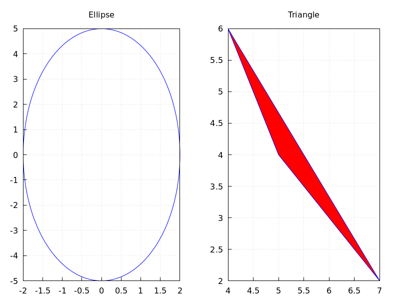
(%i1) scene1: gr2d(title="A sinus", grid=true, explicit(sin(t),t,0,2*%pi))$ (%i2) scene2: gr2d(title="A cosinus", grid=true, explicit(cos(t),t,0,2*%pi))$ (%i3) draw(scene1, scene2)$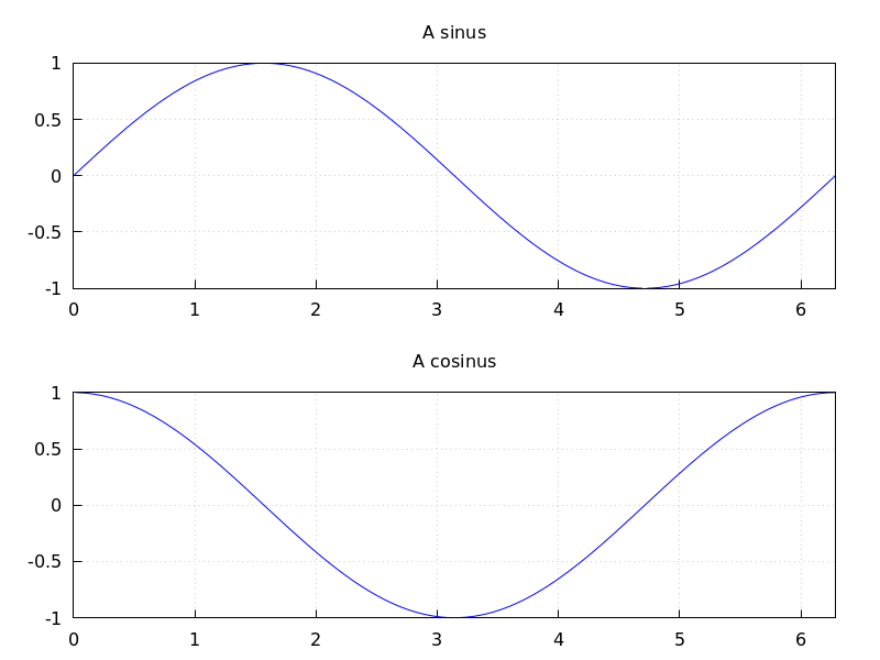
The following two draw sentences are equivalent:
(%i1) draw(gr3d(explicit(x^2+y^2,x,-1,1,y,-1,1))); (%o1) [gr3d(explicit)] (%i2) draw3d(explicit(x^2+y^2,x,-1,1,y,-1,1)); (%o2) [gr3d(explicit)]
Creating an animated gif file:
(%i1) draw( delay = 100, file_name = "zzz", terminal = 'animated_gif, gr2d(explicit(x^2,x,-1,1)), gr2d(explicit(x^3,x,-1,1)), gr2d(explicit(x^4,x,-1,1))); End of animation sequence (%o1) [gr2d(explicit), gr2d(explicit), gr2d(explicit)]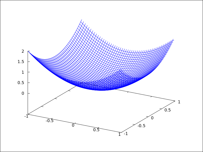
See also
gr2d,gr3d,draw2danddraw3d.Categories: Package draw · File output ·
- Function: draw2d (argument_1, ...) 
-
This function is a shortcut for
draw(gr2d(options, ..., graphic_object, ...)).It can be used to plot a unique scene in 2d, as can be seen in most examples below.
Categories: Package draw · File output ·
- Function: draw3d (argument_1, ...) 
-
This function is a shortcut for
draw(gr3d(options, ..., graphic_object, ...)).It can be used to plot a unique scene in 3d, as can be seen in many examples below.
Categories: Package draw · File output ·
- Function: draw_file (graphic option, ..., graphic object, ...) 
-
Saves the current plot into a file. Accepted graphics options are:
terminal,dimensionsandfile_name.Example:
(%i1) /* screen plot */ draw(gr3d(explicit(x^2+y^2,x,-1,1,y,-1,1)))$ (%i2) /* same plot in eps format */ draw_file(terminal = eps, dimensions = [5,5]) $Categories: Package draw · File output ·
- Function: multiplot_mode (term) 
-
This function enables Maxima to work in one-window multiplot mode with terminal term; accepted arguments for this function are
screen,wxt,aquaterm,windowsandnone.When multiplot mode is enabled, each call to
drawsends a new plot to the same window, without erasing the previous ones. To disable the multiplot mode, writemultiplot_mode(none).When multiplot mode is enabled, global option
terminalis blocked and you have to disable this working mode before changing to another terminal.On Windows this feature requires Gnuplot 5.0 or newer. Note, that just plotting multiple expressions into the same plot doesn’t require multiplot: It can be done by just issuing multiple
explicitor similar commands in a row.Example:
(%i1) set_draw_defaults( xrange = [-1,1], yrange = [-1,1], grid = true, title = "Step by step plot" )$ (%i2) multiplot_mode(screen)$ (%i3) draw2d(color=blue, explicit(x^2,x,-1,1))$ (%i4) draw2d(color=red, explicit(x^3,x,-1,1))$ (%i5) draw2d(color=brown, explicit(x^4,x,-1,1))$ (%i6) multiplot_mode(none)$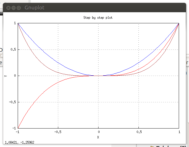 Categories: Package draw · File output ·
- Function: set_draw_defaults (graphic option, ..., graphic object, ...) 
-
Sets user graphics options. This function is useful for plotting a sequence of graphics with common graphics options. Calling this function without arguments removes user defaults.
Example:
(%i1) set_draw_defaults( xrange = [-10,10], yrange = [-2, 2], color = blue, grid = true)$ (%i2) /* plot with user defaults */ draw2d(explicit(((1+x)**2/(1+x*x))-1,x,-10,10))$ (%i3) set_draw_defaults()$ (%i4) /* plot with standard defaults */ draw2d(explicit(((1+x)**2/(1+x*x))-1,x,-10,10))$Categories: Package draw ·
55.2.3 Plot options for draw programs
- Graphic option: adapt_depth 
Default value: 10
adapt_depthis the maximum number of splittings used by the adaptive plotting routine.This option is relevant only for 2d
explicitfunctions.See also
nticksCategories: Package draw ·
- Graphic option: allocation 
Default value:
falseWith option
allocationit is possible to place a scene in the output window at will; this is of interest in multiplots. Whenfalse, the scene is placed automatically, depending on the value assigned to optioncolumns. In any other case,allocationmust be set to a list of two pairs of numbers; the first corresponds to the position of the lower left corner of the scene, and the second pair gives the width and height of the plot. All quantities must be given in relative coordinates, between 0 and 1.Examples:
In site graphics.
(%i1) draw( gr2d( explicit(x^2,x,-1,1)), gr2d( allocation = [[1/4, 1/4],[1/2, 1/2]], explicit(x^3,x,-1,1), grid = true) ) $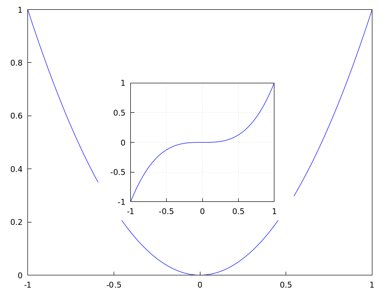
Multiplot with selected dimensions.
(%i1) draw( terminal = wxt, gr2d( grid=[5,5], allocation = [[0, 0],[1, 1/4]], explicit(x^2,x,-1,1)), gr3d( allocation = [[0, 1/4],[1, 3/4]], explicit(x^2+y^2,x,-1,1,y,-1,1) ))$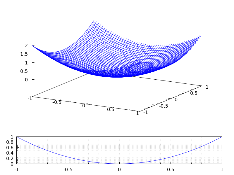
See also option
columns.Categories: Package draw ·
- Graphic option: axis_3d 
Default value:
trueIf
axis_3distrue, the x, y and z axis are shown in 3d scenes.Since this is a global graphics option, its position in the scene description does not matter.
Example:
(%i1) draw3d(axis_3d = false, explicit(sin(x^2+y^2),x,-2,2,y,-2,2) )$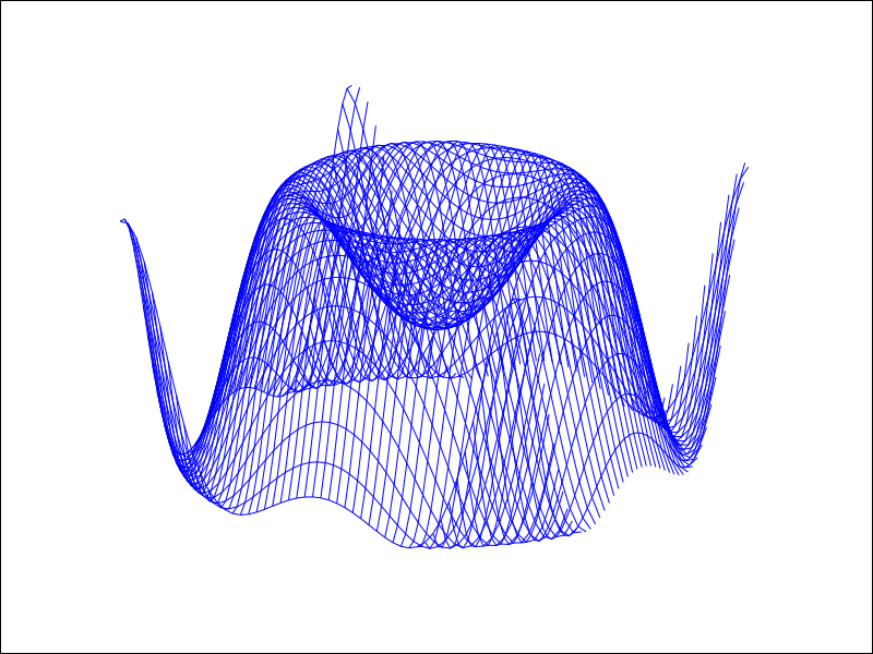
See also
axis_bottom,axis_left,axis_top, andaxis_rightfor axis in 2d.Categories: Package draw ·
- Graphic option: axis_bottom 
Default value:
trueIf
axis_bottomistrue, the bottom axis is shown in 2d scenes.Since this is a global graphics option, its position in the scene description does not matter.
Example:
(%i1) draw2d(axis_bottom = false, explicit(x^3,x,-1,1))$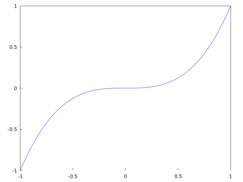
See also
axis_left,axis_top,axis_rightandaxis_3d.Categories: Package draw ·
- Graphic option: axis_left 
Default value:
trueIf
axis_leftistrue, the left axis is shown in 2d scenes.Since this is a global graphics option, its position in the scene description does not matter.
Example:
(%i1) draw2d(axis_left = false, explicit(x^3,x,-1,1))$See also
axis_bottom,axis_top,axis_rightandaxis_3d.Categories: Package draw ·
- Graphic option: axis_right 
Default value:
trueIf
axis_rightistrue, the right axis is shown in 2d scenes.Since this is a global graphics option, its position in the scene description does not matter.
Example:
(%i1) draw2d(axis_right = false, explicit(x^3,x,-1,1))$See also
axis_bottom,axis_left,axis_topandaxis_3d.Categories: Package draw ·
- Graphic option: axis_top 
Default value:
trueIf
axis_topistrue, the top axis is shown in 2d scenes.Since this is a global graphics option, its position in the scene description does not matter.
Example:
(%i1) draw2d(axis_top = false, explicit(x^3,x,-1,1))$See also
axis_bottom,axis_left,axis_right, andaxis_3d.Categories: Package draw ·
- Graphic option: background_color 
Default value:
whiteSets the background color for terminals. Default background color is white.
Since this is a global graphics option, its position in the scene description does not matter.
This option does not work with terminals
epslatexandepslatex_standalone.See also
colorCategories: Package draw ·
- Graphic option: border 
Default value:
trueIf
borderistrue, borders of polygons are painted according toline_typeandline_width.This option affects the following graphic objects:
Example:
(%i1) draw2d(color = brown, line_width = 8, polygon([[3,2],[7,2],[5,5]]), border = false, fill_color = blue, polygon([[5,2],[9,2],[7,5]]) )$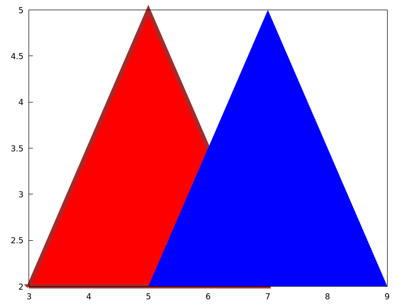 Categories: Package draw ·
- Graphic option: capping 
Default value:
[false, false]A list with two possible elements,
trueandfalse, indicating whether the extremes of a graphic objecttuberemain closed or open. By default, both extremes are left open.Setting
capping = falseis equivalent tocapping = [false, false], andcapping = trueis equivalent tocapping = [true, true].Example:
(%i1) draw3d( capping = [false, true], tube(0, 0, a, 1, a, 0, 8) )$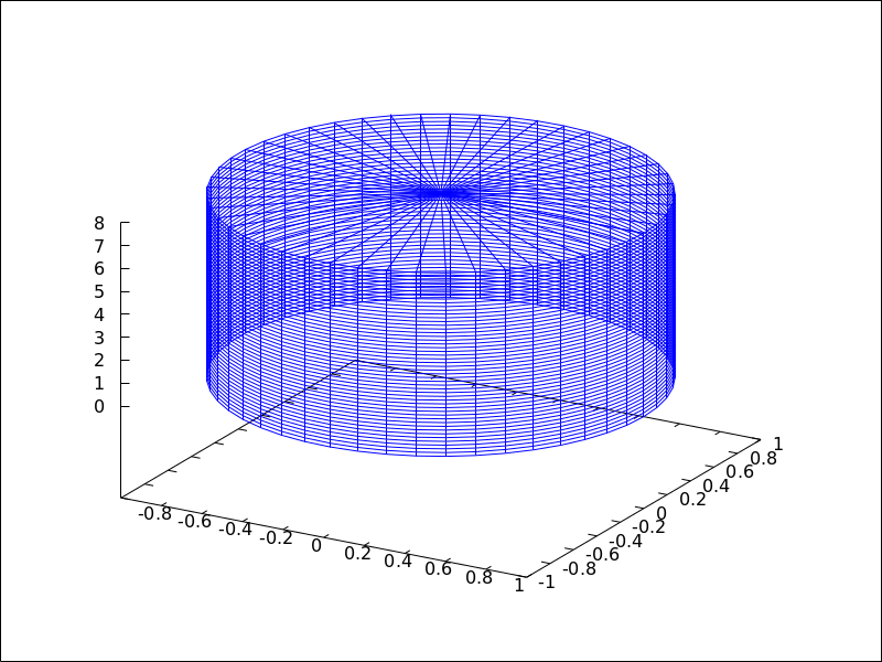 Categories: Package draw ·
- Graphic option: cbrange 
Default value:
autoIf
cbrangeisauto, the range for the values which are colored whenenhanced3dis notfalseis computed automatically. Values outside of the color range use color of the nearest extreme.When
enhanced3dorcolorboxisfalse, optioncbrangehas no effect.If the user wants a specific interval for the colored values, it must be given as a Maxima list, as in
cbrange=[-2, 3].Since this is a global graphics option, its position in the scene description does not matter.
Example:
(%i1) draw3d ( enhanced3d = true, color = green, cbrange = [-3,10], explicit(x^2+y^2, x,-2,2,y,-2,2)) $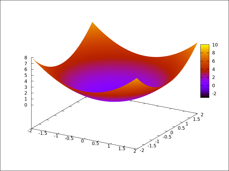
See also
enhanced3d,colorboxandcbtics.Categories: Package draw ·
- Graphic option: cbtics 
Default value:
autoThis graphic option controls the way tic marks are drawn on the colorbox when option
enhanced3dis notfalse.When
enhanced3dorcolorboxisfalse, optioncbticshas no effect.See
xticsfor a complete description.Example :
(%i1) draw3d ( enhanced3d = true, color = green, cbtics = {["High",10],["Medium",05],["Low",0]}, cbrange = [0, 10], explicit(x^2+y^2, x,-2,2,y,-2,2)) $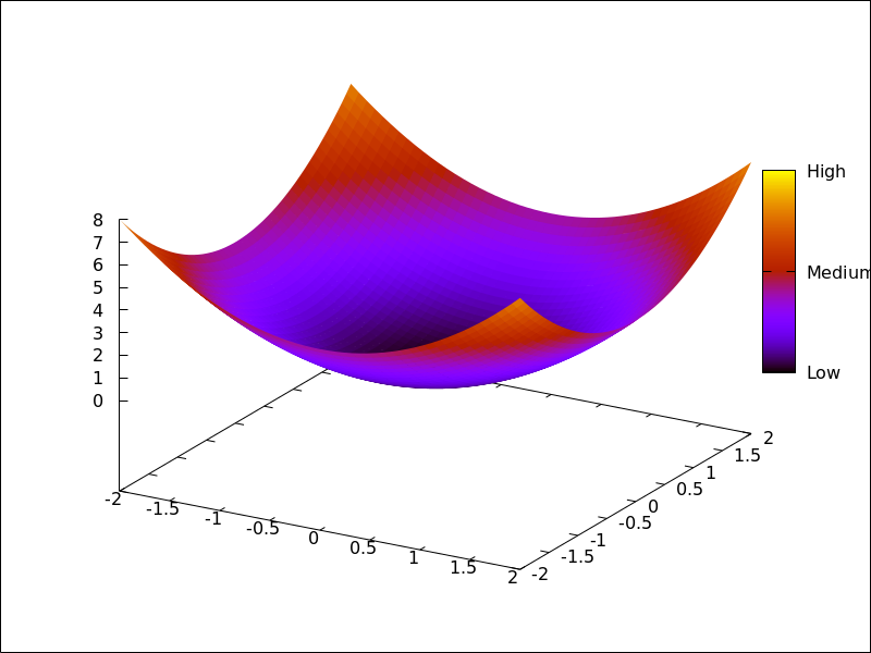
See also
enhanced3d,colorboxandcbrange.Categories: Package draw ·
- Graphic option: color 
Default value:
bluecolorspecifies the color for plotting lines, points, borders of polygons and labels.Colors can be given as names or in hexadecimal rgb code. If a gnuplot version
>= 5.0is used and the terminal that is in use supports this rgba colors with transparency information are also supported.Available color names are:
white black gray0 grey0 gray10 grey10 gray20 grey20 gray30 grey30 gray40 grey40 gray50 grey50 gray60 grey60 gray70 grey70 gray80 grey80 gray90 grey90 gray100 grey100 gray grey light_gray light_grey dark_gray dark_grey red light_red dark_red yellow light_yellow dark_yellow green light_green dark_green spring_green forest_green sea_green blue light_blue dark_blue midnight_blue navy medium_blue royalblue skyblue cyan light_cyan dark_cyan magenta light_magenta dark_magenta turquoise light_turquoise dark_turquoise pink light_pink dark_pink coral light_coral orange_red salmon light_salmon dark_salmon aquamarine khaki dark_khaki goldenrod light_goldenrod dark_goldenrod gold beige brown orange dark_orange violet dark_violet plum purple
Cromatic components in hexadecimal code are introduced in the form
"#rrggbb".Example:
(%i1) draw2d(explicit(x^2,x,-1,1), /* default is black */ color = red, explicit(0.5 + x^2,x,-1,1), color = blue, explicit(1 + x^2,x,-1,1), color = light_blue, explicit(1.5 + x^2,x,-1,1), color = "#23ab0f", label(["This is a label",0,1.2]) )$
(%i1) draw2d( line_width=50, color="#FF0000", explicit(sin(x),x,0,10), color="#0000FF80", explicit(cos(x),x,0,10) );
(%i1) H(p,p_0) := %i/(2*%pi*(p-p_0))$ (%i2) draw2d( proportional_axes=xy, ip_grid=[150,150], grid=true, makelist( [ color=printf(false,"#~2,'0x~2,'0x~2,'0x",i*10,0,0), key_pos=top_left, key = if mod(i,5)=0 then sconcat("H=",i,"A/M") else "", implicit( cabs(H(x+%i*y,-1-%i)+H(x+%i*y,1+%i)-H(x+%i*y,1-%i) -H(x+%i*y,-1+%i))=i/10, x,-3,3, y,-3,3 ) ], i,1,25 ) )$
(%i1) draw2d( "figures/draw_color4", makelist( [ color=i, key=sconcat("color =",i), explicit(sin(i*x),x,0,1) ], i,0,17 ) )$
See also
fill_color.Categories: Package draw ·
- Graphic option: colorbox 
Default value:
trueIf
colorboxistrue, a color scale without label is drawn together withimage2D objects, or coloured 3d objects. Ifcolorboxisfalse, no color scale is shown. Ifcolorboxis a string, a color scale with label is drawn.Since this is a global graphics option, its position in the scene description does not matter.
Example:
Color scale and images.
(%i1) im: apply('matrix, makelist(makelist(random(200),i,1,30),i,1,30))$ (%i2) draw( gr2d(image(im,0,0,30,30)), gr2d(colorbox = false, image(im,0,0,30,30)) )$
Color scale and 3D coloured object.
(%i1) draw3d( colorbox = "Magnitude", enhanced3d = true, explicit(x^2+y^2,x,-1,1,y,-1,1))$
See also
palette_draw.Categories: Package draw ·
- Graphic option: columns 
Default value: 1
columnsis the number of columns in multiple plots.Since this is a global graphics option, its position in the scene description does not matter. It can be also used as an argument of function
draw.Example:
(%i1) scene1: gr2d(title="Ellipse", nticks=30, parametric(2*cos(t),5*sin(t),t,0,2*%pi))$ (%i2) scene2: gr2d(title="Triangle", polygon([4,5,7],[6,4,2]))$ (%i3) draw(scene1, scene2, columns = 2)$ Categories: Package draw ·
- Graphic option: contour 
Default value:
noneOption
contourenables the user to select where to plot contour lines. Possible values are:-
none: no contour lines are plotted. -
base: contour lines are projected on the xy plane. -
surface: contour lines are plotted on the surface. -
both: two contour lines are plotted: on the xy plane and on the surface. -
map: contour lines are projected on the xy plane, and the view point is set just in the vertical.
Since this is a global graphics option, its position in the scene description does not matter.
Example:
(%i1) draw3d(explicit(20*exp(-x^2-y^2)-10,x,0,2,y,-3,3), contour_levels = 15, contour = both, surface_hide = true) $
(%i1) draw3d(explicit(20*exp(-x^2-y^2)-10,x,0,2,y,-3,3), contour_levels = 15, contour = map ) $ Categories: Package draw ·
-
- Graphic option: contour_levels 
Default value: 5
This graphic option controls the way contours are drawn.
contour_levelscan be set to a positive integer number, a list of three numbers or an arbitrary set of numbers:- When option
contour_levelsis bounded to positive integer n, n contour lines will be drawn at equal intervals. By default, five equally spaced contours are plotted. - When option
contour_levelsis bounded to a list of length three of the form[lowest,s,highest], contour lines are plotted fromlowesttohighestin steps ofs. - When option
contour_levelsis bounded to a set of numbers of the form{n1, n2, ...}, contour lines are plotted at valuesn1,n2, ...
Since this is a global graphics option, its position in the scene description does not matter.
Examples:
Ten equally spaced contour lines. The actual number of levels can be adjusted to give simple labels.
(%i1) draw3d(color = green, explicit(20*exp(-x^2-y^2)-10,x,0,2,y,-3,3), contour_levels = 10, contour = both, surface_hide = true) $From -8 to 8 in steps of 4.
(%i1) draw3d(color = green, explicit(20*exp(-x^2-y^2)-10,x,0,2,y,-3,3), contour_levels = [-8,4,8], contour = both, surface_hide = true) $Isolines at levels -7, -6, 0.8 and 5.
(%i1) draw3d(color = green, explicit(20*exp(-x^2-y^2)-10,x,0,2,y,-3,3), contour_levels = {-7, -6, 0.8, 5}, contour = both, surface_hide = true) $See also
contour.Categories: Package draw ·- When option
- Graphic option: data_file_name 
Default value:
"data.gnuplot"This is the name of the file with the numeric data needed by Gnuplot to build the requested plot.
Since this is a global graphics option, its position in the scene description does not matter. It can be also used as an argument of function
draw.See example in
gnuplot_file_name.Categories: Package draw ·
- Graphic option: delay 
Default value: 5
This is the delay in 1/100 seconds of frames in animated gif files.
Since this is a global graphics option, its position in the scene description does not matter. It can be also used as an argument of function
draw.Example:
(%i1) draw( delay = 100, file_name = "zzz", terminal = 'animated_gif, gr2d(explicit(x^2,x,-1,1)), gr2d(explicit(x^3,x,-1,1)), gr2d(explicit(x^4,x,-1,1))); End of animation sequence (%o2) [gr2d(explicit), gr2d(explicit), gr2d(explicit)]Option
delayis only active in animated gif’s; it is ignored in any other case.See also
terminal, anddimensions.Categories: Package draw ·
- Graphic option: dimensions 
Default value:
[600,500]Dimensions of the output terminal. Its value is a list formed by the width and the height. The meaning of the two numbers depends on the terminal you are working with.
With terminals
gif,animated_gif,png,jpg,svg,screen,wxt,qt,x11,windowsandaquaterm, the integers represent the number of points in each direction. If they are not integers, they are rounded.With terminals
eps,epslatex,epslatex_standalone,eps_color,multipage_eps,multipage_eps_color,cairolatex_pdf,cairolatex_pdf_standalone,pdf,multipage_pdf,pdfcairo,multipage_pdfcairo,tikz, andtikz_standalone, both numbers represent hundredths of cm, which means that, by default, pictures in these formats are 6 cm in width and 5 cm in height.Since this is a global graphics option, its position in the scene description does not matter. It can be also used as an argument of function
draw.Examples:
Option
dimensionsapplied to file output and to wxt canvas.(%i1) draw2d( dimensions = [300,300], terminal = 'png, explicit(x^4,x,-1,1)) $ (%i2) draw2d( dimensions = [300,300], terminal = 'wxt, explicit(x^4,x,-1,1)) $Option
dimensionsapplied to eps output. We want an eps file with A4 portrait dimensions.(%i1) A4portrait: 100*[21, 29.7]$ (%i2) draw3d( dimensions = A4portrait, terminal = 'eps, explicit(x^2-y^2,x,-2,2,y,-2,2)) $Categories: Package draw ·
- Graphic option: draw_realpart 
Default value:
trueWhen
true, functions to be drawn are considered as complex functions whose real part value should be plotted; whenfalse, nothing will be plotted when the function does not give a real value.This option affects objects
explicitandparametricin 2D and 3D, andparametric_surface.Example:
(%i1) draw2d( draw_realpart = false, explicit(sqrt(x^2 - 4*x) - x, x, -1, 5), color = red, draw_realpart = true, parametric(x,sqrt(x^2 - 4*x) - x + 1, x, -1, 5) );Categories: Package draw ·
- Graphic option: enhanced3d 
Default value:
noneIf
enhanced3disnone, surfaces are not colored in 3D plots. In order to get a colored surface, a list must be assigned to optionenhanced3d, where the first element is an expression and the rest are the names of the variables or parameters used in that expression. A list such[f(x,y,z), x, y, z]means that point[x,y,z]of the surface is assigned numberf(x,y,z), which will be colored according to the actualpalette. For those 3D graphic objects defined in terms of parameters, it is possible to define the color number in terms of the parameters, as in[f(u), u], as in objectsparametricandtube, or[f(u,v), u, v], as in objectparametric_surface. While all 3D objects admit the model based on absolute coordinates,[f(x,y,z), x, y, z], only two of them, namelyexplicitandelevation_grid, accept also models defined on the[x,y]coordinates,[f(x,y), x, y]. 3D graphic objectimplicitaccepts only the[f(x,y,z), x, y, z]model. Objectpointsaccepts also the[f(x,y,z), x, y, z]model, but when points have a chronological nature, model[f(k), k]is also valid, beingkan ordering parameter.When
enhanced3dis assigned something different tonone, optionscolorandsurface_hideare ignored.The names of the variables defined in the lists may be different to those used in the definitions of the graphic objects.
In order to maintain back compatibility,
enhanced3d = falseis equivalent toenhanced3d = none, andenhanced3d = trueis equivalent toenhanced3d = [z, x, y, z]. If an expression is given toenhanced3d, its variables must be the same used in the surface definition. This is not necessary when using lists.See option
paletteto learn how palettes are specified.Examples:
explicitobject with coloring defined by the[f(x,y,z), x, y, z]model.(%i1) draw3d( enhanced3d = [x-z/10,x,y,z], palette = gray, explicit(20*exp(-x^2-y^2)-10,x,-3,3,y,-3,3))$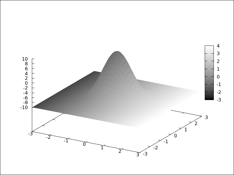
explicitobject with coloring defined by the[f(x,y), x, y]model. The names of the variables defined in the lists may be different to those used in the definitions of the graphic objects; in this case,rcorresponds tox, andstoy.(%i1) draw3d( enhanced3d = [sin(r*s),r,s], explicit(20*exp(-x^2-y^2)-10,x,-3,3,y,-3,3))$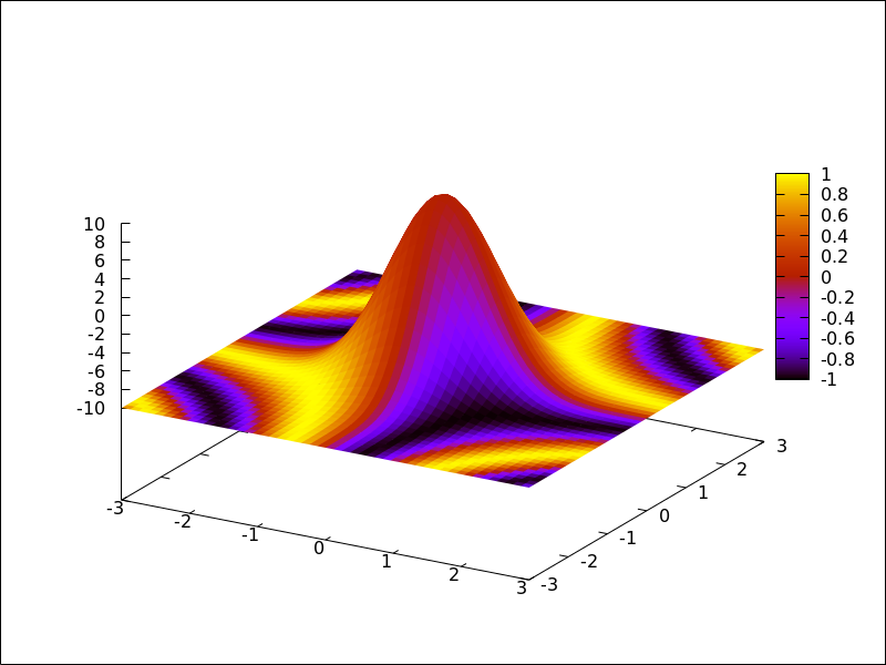
parametricobject with coloring defined by the[f(x,y,z), x, y, z]model.(%i1) draw3d( nticks = 100, line_width = 2, enhanced3d = [if y>= 0 then 1 else 0, x, y, z], parametric(sin(u)^2,cos(u),u,u,0,4*%pi)) $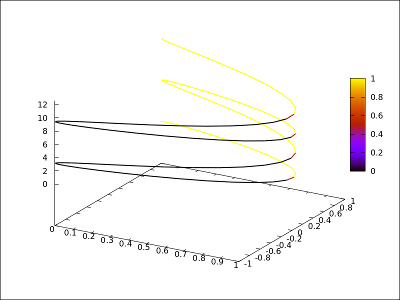
parametricobject with coloring defined by the[f(u), u]model. In this case,(u-1)^2is a shortcut for[(u-1)^2,u].(%i1) draw3d( nticks = 60, line_width = 3, enhanced3d = (u-1)^2, parametric(cos(5*u)^2,sin(7*u),u-2,u,0,2))$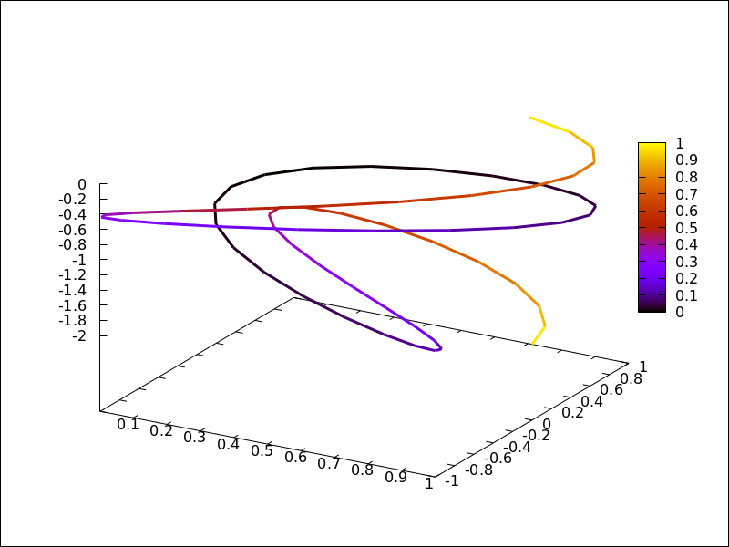
elevation_gridobject with coloring defined by the[f(x,y), x, y]model.(%i1) m: apply( matrix, makelist(makelist(cos(i^2/80-k/30),k,1,30),i,1,20)) $ (%i2) draw3d( enhanced3d = [cos(x*y*10),x,y], elevation_grid(m,-1,-1,2,2), xlabel = "x", ylabel = "y");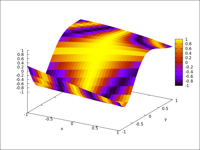
tubeobject with coloring defined by the[f(x,y,z), x, y, z]model.(%i1) draw3d( enhanced3d = [cos(x-y),x,y,z], palette = gray, xu_grid = 50, tube(cos(a), a, 0, 1, a, 0, 4*%pi) )$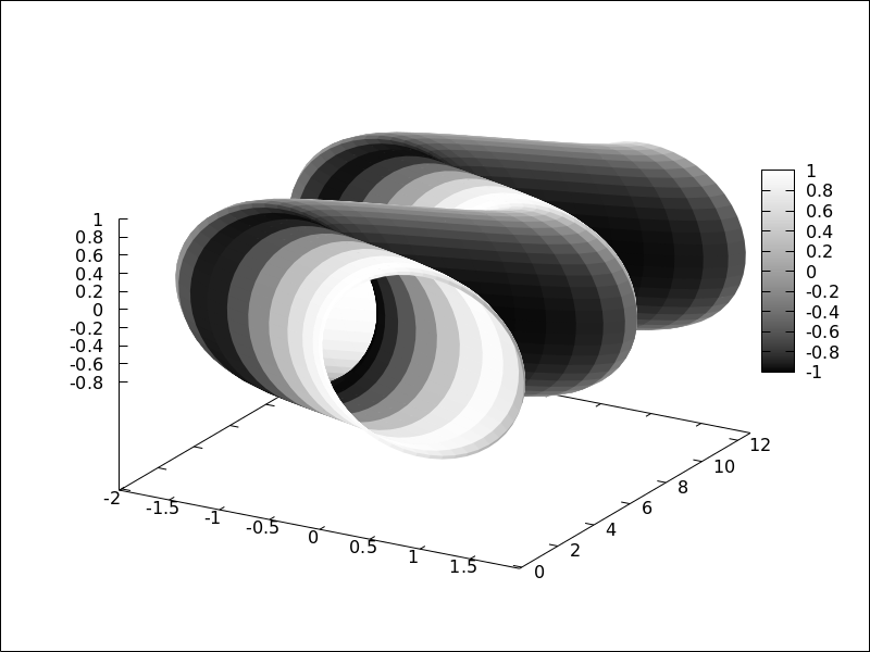
tubeobject with coloring defined by the[f(u), u]model. Here,enhanced3d = -awould be the shortcut forenhanced3d = [-foo,foo].(%i1) draw3d( capping = [true, false], palette = [26,15,-2], enhanced3d = [-foo, foo], tube(a, a, a^2, 1, a, -2, 2) )$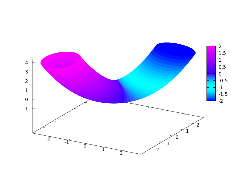
implicitandpointsobjects with coloring defined by the[f(x,y,z), x, y, z]model.(%i1) draw3d( enhanced3d = [x-y,x,y,z], implicit((x^2+y^2+z^2-1)*(x^2+(y-1.5)^2+z^2-0.5)=0.015, x,-1,1,y,-1.2,2.3,z,-1,1)) $ (%i2) m: makelist([random(1.0),random(1.0),random(1.0)],k,1,2000)$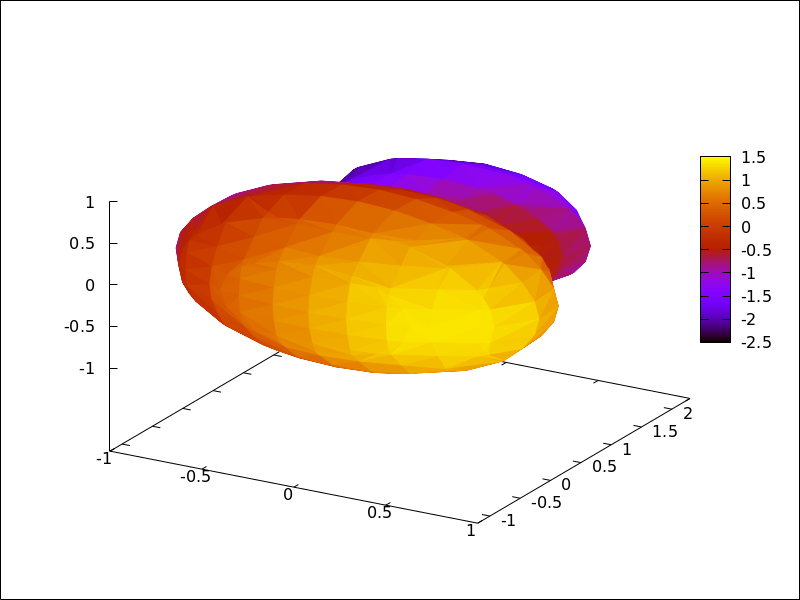
(%i3) draw3d( point_type = filled_circle, point_size = 2, enhanced3d = [u+v-w,u,v,w], points(m) ) $
When points have a chronological nature, model
[f(k), k]is also valid, beingkan ordering parameter.(%i1) m:makelist([random(1.0), random(1.0), random(1.0)],k,1,5)$ (%i2) draw3d( enhanced3d = [sin(j), j], point_size = 3, point_type = filled_circle, points_joined = true, points(m)) $ Categories: Package draw ·
- Graphic option: error_type 
Default value:
yDepending on its value, which can be
x,y, orxy, graphic objecterrorswill draw points with horizontal, vertical, or both, error bars. Whenerror_type=boxes, boxes will be drawn instead of crosses.See also
errors.
- Graphic option: file_name 
Default value:
"maxima_out"This is the name of the file where terminals
png,jpg,gif,eps,eps_color,pdf,pdfcairoandsvgwill save the graphic.Since this is a global graphics option, its position in the scene description does not matter. It can be also used as an argument of function
draw.Example:
(%i1) draw2d(file_name = "myfile", explicit(x^2,x,-1,1), terminal = 'png)$See also
terminal,dimensions_draw.Categories: Package draw ·
- Graphic option: fill_color 
Default value:
"red"fill_colorspecifies the color for filling polygons and 2dexplicitfunctions.See
colorto learn how colors are specified.Categories: Package draw ·
- Graphic option: fill_density 
Default value: 0
fill_densityis a number between 0 and 1 that specifies the intensity of thefill_colorinbarsobjects.See
barsfor examples.
- Graphic option: filled_func 
Default value:
falseOption
filled_funccontrols how regions limited by functions should be filled. Whenfilled_funcistrue, the region bounded by the function defined with objectexplicitand the bottom of the graphic window is filled withfill_color. Whenfilled_funccontains a function expression, then the region bounded by this function and the function defined with objectexplicitwill be filled. By default, explicit functions are not filled.A useful special case is
filled_func=0, which generates the region bond by the horizontal axis and the explicit function.This option affects only the 2d graphic object
explicit.Example:
Region bounded by an
explicitobject and the bottom of the graphic window.(%i1) draw2d(fill_color = red, filled_func = true, explicit(sin(x),x,0,10) )$
Region bounded by an
explicitobject and the function defined by optionfilled_func. Note that the variable infilled_funcmust be the same as that used inexplicit.(%i1) draw2d(fill_color = grey, filled_func = sin(x), explicit(-sin(x),x,0,%pi));
See also
fill_colorandexplicit.Categories: Package draw ·
- Graphic option: font 
Default value:
""(empty string)This option can be used to set the font face to be used by the terminal. Only one font face and size can be used throughout the plot.
Since this is a global graphics option, its position in the scene description does not matter.
See also
font_size.Gnuplot doesn’t handle fonts by itself, it leaves this task to the support libraries of the different terminals, each one with its own philosophy about it. A brief summary follows:
- x11:
Uses the normal x11 font server mechanism.
Example:
(%i1) draw2d(font = "Arial", font_size = 20, label(["Arial font, size 20",1,1]))$ - windows: The windows terminal doesn’t support changing of fonts from inside the plot. Once the plot has been generated, the font can be changed right-clicking on the menu of the graph window.
- png, jpeg, gif:
The libgd library uses the font path stored in the environment
variable
GDFONTPATH; in this case, it is only necessary to set optionfontto the font’s name. It is also possible to give the complete path to the font file.Examples:
Option
fontcan be given the complete path to the font file:(%i1) path: "/usr/share/fonts/truetype/freefont/" $ (%i2) file: "FreeSerifBoldItalic.ttf" $ (%i3) draw2d( font = concat(path, file), font_size = 20, color = red, label(["FreeSerifBoldItalic font, size 20",1,1]), terminal = png)$If environment variable
GDFONTPATHis set to the path where font files are allocated, it is possible to set graphic optionfontto the name of the font.(%i1) draw2d( font = "FreeSerifBoldItalic", font_size = 20, color = red, label(["FreeSerifBoldItalic font, size 20",1,1]), terminal = png)$ - Postscript:
Standard Postscript fonts are:
"Times-Roman","Times-Italic","Times-Bold","Times-BoldItalic",
"Helvetica","Helvetica-Oblique","Helvetica-Bold",
"Helvetic-BoldOblique","Courier","Courier-Oblique","Courier-Bold",
and"Courier-BoldOblique".Example:
(%i1) draw2d( font = "Courier-Oblique", font_size = 15, label(["Courier-Oblique font, size 15",1,1]), terminal = eps)$ - pdf: Uses same fonts as Postscript.
- pdfcairo: Uses same fonts as wxt.
- wxt:
The pango library finds fonts via the
fontconfigutility. - aqua:
Default is
"Times-Roman".
The gnuplot documentation is an important source of information about terminals and fonts.
Categories: Package draw ·- x11:
Uses the normal x11 font server mechanism.
- Graphic option: font_size 
Default value: 10
This option can be used to set the font size to be used by the terminal. Only one font face and size can be used throughout the plot.
font_sizeis active only when optionfontis not equal to the empty string.Since this is a global graphics option, its position in the scene description does not matter.
See also
font.Categories: Package draw ·
- Graphic option: gnuplot_file_name 
Default value:
"maxout_xxx.gnuplot"with"xxx"being a number that is unique to each concurrently-running maxima process.This is the name of the file with the necessary commands to be processed by Gnuplot.
Since this is a global graphics option, its position in the scene description does not matter. It can be also used as an argument of function
draw.Example:
(%i1) draw2d( file_name = "my_file", gnuplot_file_name = "my_commands_for_gnuplot", data_file_name = "my_data_for_gnuplot", terminal = png, explicit(x^2,x,-1,1)) $See also
data_file_name.Categories: Package draw ·
- Graphic option: grid 
Default value:
falseIf
gridisnot false, a grid will be drawn on the xy plane. Ifgridis assigned true, one grid line per tick of each axis is drawn. Ifgridis assigned a listnx,nywith[nx,ny] > [0,0]insteadnxlines per tick of the x axis andnylines per tick of the y axis are drawn.Since this is a global graphics option, its position in the scene description does not matter.
Example:
(%i1) draw2d(grid = true, explicit(exp(u),u,-2,2))$
(%i1) draw2d(grid = [2,2], explicit(sin(x),x,0,2*%pi))$ Categories: Package draw ·
- Graphic option: head_angle 
Default value: 45
head_angleindicates the angle, in degrees, between the arrow heads and the segment.This option is relevant only for
vectorobjects.Example:
(%i1) draw2d(xrange = [0,10], yrange = [0,9], head_length = 0.7, head_angle = 10, vector([1,1],[0,6]), head_angle = 20, vector([2,1],[0,6]), head_angle = 30, vector([3,1],[0,6]), head_angle = 40, vector([4,1],[0,6]), head_angle = 60, vector([5,1],[0,6]), head_angle = 90, vector([6,1],[0,6]), head_angle = 120, vector([7,1],[0,6]), head_angle = 160, vector([8,1],[0,6]), head_angle = 180, vector([9,1],[0,6]) )$
See also
head_both,head_length, andhead_type.Categories: Package draw ·
- Graphic option: head_both 
Default value:
falseIf
head_bothistrue, vectors are plotted with two arrow heads. Iffalse, only one arrow is plotted.This option is relevant only for
vectorobjects.Example:
(%i1) draw2d(xrange = [0,8], yrange = [0,8], head_length = 0.7, vector([1,1],[6,0]), head_both = true, vector([1,7],[6,0]) )$
See also
head_length,head_angle, andhead_type.Categories: Package draw ·
- Graphic option: head_length 
Default value: 2
head_lengthindicates, in x-axis units, the length of arrow heads.This option is relevant only for
vectorobjects.Example:
(%i1) draw2d(xrange = [0,12], yrange = [0,8], vector([0,1],[5,5]), head_length = 1, vector([2,1],[5,5]), head_length = 0.5, vector([4,1],[5,5]), head_length = 0.25, vector([6,1],[5,5]))$
See also
head_both,head_angle, andhead_type.Categories: Package draw ·
- Graphic option: head_type 
Default value:
filledhead_typeis used to specify how arrow heads are plotted. Possible values are:filled(closed and filled arrow heads),empty(closed but not filled arrow heads), andnofilled(open arrow heads).This option is relevant only for
vectorobjects.Example:
(%i1) draw2d(xrange = [0,12], yrange = [0,10], head_length = 1, vector([0,1],[5,5]), /* default type */ head_type = 'empty, vector([3,1],[5,5]), head_type = 'nofilled, vector([6,1],[5,5]))$
See also
head_both,head_angle, andhead_length.Categories: Package draw ·
- Graphic option: interpolate_color 
Default value:
falseThis option is relevant only when
enhanced3dis notfalse.When
interpolate_colorisfalse, surfaces are colored with homogeneous quadrangles. Whentrue, color transitions are smoothed by interpolation.interpolate_coloralso accepts a list of two numbers,[m,n]. For positive m and n, each quadrangle or triangle is interpolated m times and n times in the respective direction. For negative m and n, the interpolation frequency is chosen so that there will be at least |m| and |n| points drawn; you can consider this as a special gridding function. Zeros, i.e.interpolate_color=[0,0], will automatically choose an optimal number of interpolated surface points.Also,
interpolate_color=trueis equivalent tointerpolate_color=[0,0].Examples:
Color interpolation with explicit functions.
(%i1) draw3d( enhanced3d = sin(x*y), explicit(20*exp(-x^2-y^2)-10, x ,-3, 3, y, -3, 3)) $
(%i2) draw3d( interpolate_color = true, enhanced3d = sin(x*y), explicit(20*exp(-x^2-y^2)-10, x ,-3, 3, y, -3, 3)) $
(%i3) draw3d( interpolate_color = [-10,0], enhanced3d = sin(x*y), explicit(20*exp(-x^2-y^2)-10, x ,-3, 3, y, -3, 3)) $
Color interpolation with the
meshgraphic object.Interpolating colors in parametric surfaces can give unexpected results.
(%i1) draw3d( enhanced3d = true, mesh([[1,1,3], [7,3,1],[12,-2,4],[15,0,5]], [[2,7,8], [4,3,1],[10,5,8], [12,7,1]], [[-2,11,10],[6,9,5],[6,15,1], [20,15,2]])) $
(%i2) draw3d( enhanced3d = true, interpolate_color = true, mesh([[1,1,3], [7,3,1],[12,-2,4],[15,0,5]], [[2,7,8], [4,3,1],[10,5,8], [12,7,1]], [[-2,11,10],[6,9,5],[6,15,1], [20,15,2]])) $
(%i3) draw3d( enhanced3d = true, interpolate_color = true, view=map, mesh([[1,1,3], [7,3,1],[12,-2,4],[15,0,5]], [[2,7,8], [4,3,1],[10,5,8], [12,7,1]], [[-2,11,10],[6,9,5],[6,15,1], [20,15,2]])) $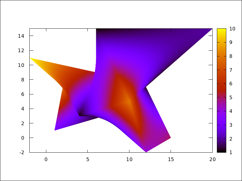
See also
enhanced3d.Categories: Package draw ·
- Graphic option: ip_grid 
Default value:
[50, 50]ip_gridsets the grid for the first sampling in implicit plots.This option is relevant only for
implicitobjects.Categories: Package draw ·
- Graphic option: ip_grid_in 
Default value:
[5, 5]ip_grid_insets the grid for the second sampling in implicit plots.This option is relevant only for
implicitobjects.Categories: Package draw ·
- Graphic option: key 
Default value:
""(empty string)keyis the name of a function in the legend. Ifkeyis an empty string, no key is assigned to the function.This option affects the following graphic objects:
-
gr2d:points,polygon,rectangle,ellipse,vector,explicit,implicit,parametricandpolar. -
gr3d:points,explicit,parametricandparametric_surface.
Example:
(%i1) draw2d(key = "Sinus", explicit(sin(x),x,0,10), key = "Cosinus", color = red, explicit(cos(x),x,0,10) )$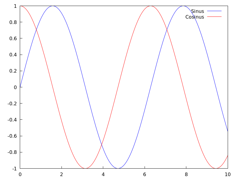 Categories: Package draw ·
-
- Graphic option: key_pos 
Default value:
""(empty string)key_posdefines at which position the legend will be drawn. Ifkeyis an empty string,"top_right"is used. Available position specifiers are:top_left,top_center,top_right,center_left,center,center_right,bottom_left,bottom_center, andbottom_right.Since this is a global graphics option, its position in the scene description does not matter.
Example:
(%i1) draw2d( key_pos = top_left, key = "x", explicit(x, x,0,10), color= red, key = "x squared", explicit(x^2,x,0,10))$ (%i3) draw3d( key_pos = center, key = "x", explicit(x+y,x,0,10,y,0,10), color= red, key = "x squared", explicit(x^2+y^2,x,0,10,y,0,10))$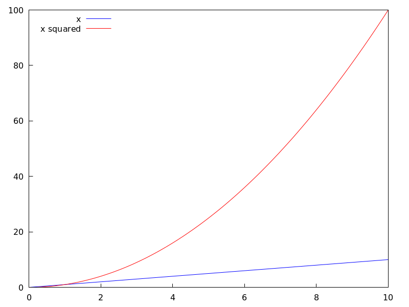 Categories: Package draw ·
- Graphic option: label_alignment 
Default value:
centerlabel_alignmentis used to specify where to write labels with respect to the given coordinates. Possible values are:center,left, andright.This option is relevant only for
labelobjects.Example:
(%i1) draw2d(xrange = [0,10], yrange = [0,10], points_joined = true, points([[5,0],[5,10]]), color = blue, label(["Centered alignment (default)",5,2]), label_alignment = 'left, label(["Left alignment",5,5]), label_alignment = 'right, label(["Right alignment",5,8]))$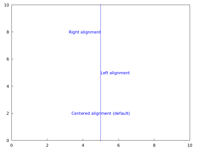
See also
label_orientation, andcolorCategories: Package draw ·
- Graphic option: label_orientation 
Default value:
horizontallabel_orientationis used to specify orientation of labels. Possible values are:horizontal, andvertical.This option is relevant only for
labelobjects.Example:
In this example, a dummy point is added to get an image. Package
drawneeds always data to draw an scene.(%i1) draw2d(xrange = [0,10], yrange = [0,10], point_size = 0, points([[5,5]]), color = navy, label(["Horizontal orientation (default)",5,2]), label_orientation = 'vertical, color = "#654321", label(["Vertical orientation",1,5]))$
See also
label_alignmentandcolorCategories: Package draw ·
- Graphic option: line_type 
Default value:
solidline_typeindicates how lines are displayed; possible values aresolidanddots, both available in all terminals, anddashes,short_dashes,short_long_dashes,short_short_long_dashes, anddot_dash, which are not available inpng,jpg, andgifterminals.This option affects the following graphic objects:
-
gr2d:points,polygon,rectangle,ellipse,vector,explicit,implicit,parametricandpolar. -
gr3d:points,explicit,parametricandparametric_surface.
Example:
(%i1) draw2d(line_type = dots, explicit(1 + x^2,x,-1,1), line_type = solid, /* default */ explicit(2 + x^2,x,-1,1))$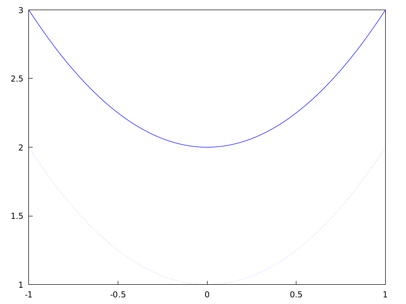
See also
line_width.Categories: Package draw ·-
- Graphic option: line_width 
Default value: 1
line_widthis the width of plotted lines. Its value must be a positive number.This option affects the following graphic objects:
-
gr2d:points,polygon,rectangle,ellipse,vector,explicit,implicit,parametricandpolar. -
gr3d:pointsandparametric.
Example:
(%i1) draw2d(explicit(x^2,x,-1,1), /* default width */ line_width = 5.5, explicit(1 + x^2,x,-1,1), line_width = 10, explicit(2 + x^2,x,-1,1))$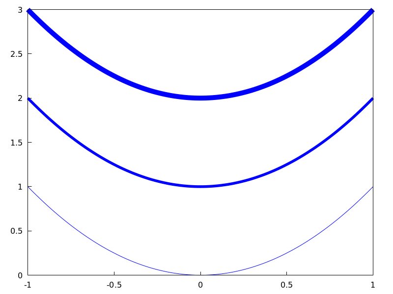
See also
line_type.Categories: Package draw ·-
- Graphic option: logcb 
Default value:
falseIf
logcbistrue, the tics in the colorbox will be drawn in the logarithmic scale.When
enhanced3dorcolorboxisfalse, optionlogcbhas no effect.Since this is a global graphics option, its position in the scene description does not matter.
Example:
(%i1) draw3d ( enhanced3d = true, color = green, logcb = true, logz = true, palette = [-15,24,-9], explicit(exp(x^2-y^2), x,-2,2,y,-2,2)) $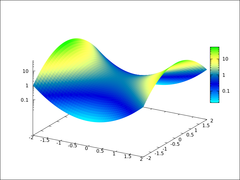
See also
enhanced3d,colorboxandcbrange.Categories: Package draw ·
- Graphic option: logx 
Default value:
falseIf
logxistrue, the x axis will be drawn in the logarithmic scale.Since this is a global graphics option, its position in the scene description does not matter, with the exception that it should be written before any 2D
explicitobject, so thatdrawcan produce a better plot.Example:
(%i1) draw2d(logx = true, explicit(log(x),x,0.01,5))$See also
logy,logx_secondary,logy_secondary, andlogz.Categories: Package draw ·
- Graphic option: logx_secondary 
Default value:
falseIf
logx_secondaryistrue, the secondary x axis will be drawn in the logarithmic scale.This option is relevant only for 2d scenes.
Since this is a global graphics option, its position in the scene description does not matter.
Example:
(%i1) draw2d( grid = true, key="x^2, linear scale", color=red, explicit(x^2,x,1,100), xaxis_secondary = true, xtics_secondary = true, logx_secondary = true, key = "x^2, logarithmic x scale", color = blue, explicit(x^2,x,1,100) )$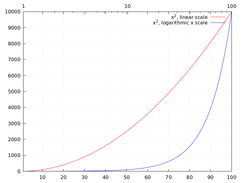
See also
logx_draw,logy_draw,logy_secondary, andlogz.Categories: Package draw ·
- Graphic option: logy 
Default value:
falseIf
logyistrue, the y axis will be drawn in the logarithmic scale.Since this is a global graphics option, its position in the scene description does not matter.
Example:
(%i1) draw2d(logy = true, explicit(exp(x),x,0,5))$See also
logx_draw,logx_secondary,logy_secondary, andlogz.Categories: Package draw ·
- Graphic option: logy_secondary 
Default value:
falseIf
logy_secondaryistrue, the secondary y axis will be drawn in the logarithmic scale.This option is relevant only for 2d scenes.
Since this is a global graphics option, its position in the scene description does not matter.
Example:
(%i1) draw2d( grid = true, key="x^2, linear scale", color=red, explicit(x^2,x,1,100), yaxis_secondary = true, ytics_secondary = true, logy_secondary = true, key = "x^2, logarithmic y scale", color = blue, explicit(x^2,x,1,100) )$See also
logx_draw,logy_draw,logx_secondary, andlogz.Categories: Package draw ·
- Graphic option: logz 
Default value:
falseIf
logzistrue, the z axis will be drawn in the logarithmic scale.Since this is a global graphics option, its position in the scene description does not matter.
Example:
(%i1) draw3d(logz = true, explicit(exp(u^2+v^2),u,-2,2,v,-2,2))$See also
logx_drawandlogy_draw.Categories: Package draw ·
- Graphic option: nticks 
Default value: 29
In 2d,
nticksgives the initial number of points used by the adaptive plotting routine for explicit objects. It is also the number of points that will be shown in parametric and polar curves.This option affects the following graphic objects:
-
gr2d:ellipse,explicit,parametricandpolar. -
gr3d:parametric.
See also
adapt_depthExample:
(%i1) draw2d(transparent = true, ellipse(0,0,4,2,0,180), nticks = 5, ellipse(0,0,4,2,180,180) )$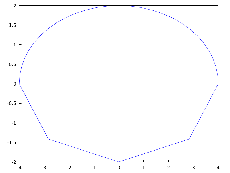 Categories: Package draw ·
-
- Graphic option: palette 
Default value:
colorpaletteindicates how to map gray levels onto color components. It works together with optionenhanced3din 3D graphics, who associates every point of a surfaces to a real number or gray level. It also works with gray images. Withpalette, levels are transformed into colors.There are two ways for defining these transformations.
First,
palettecan be a vector of length three with components ranging from -36 to +36; each value is an index for a formula mapping the levels onto red, green and blue colors, respectively:0: 0 1: 0.5 2: 1 3: x 4: x^2 5: x^3 6: x^4 7: sqrt(x) 8: sqrt(sqrt(x)) 9: sin(90x) 10: cos(90x) 11: |x-0.5| 12: (2x-1)^2 13: sin(180x) 14: |cos(180x)| 15: sin(360x) 16: cos(360x) 17: |sin(360x)| 18: |cos(360x)| 19: |sin(720x)| 20: |cos(720x)| 21: 3x 22: 3x-1 23: 3x-2 24: |3x-1| 25: |3x-2| 26: (3x-1)/2 27: (3x-2)/2 28: |(3x-1)/2| 29: |(3x-2)/2| 30: x/0.32-0.78125 31: 2*x-0.84 32: 4x;1;-2x+1.84;x/0.08-11.5 33: |2*x - 0.5| 34: 2*x 35: 2*x - 0.5 36: 2*x - 1
negative numbers mean negative colour component.
palette = grayandpalette = colorare short cuts forpalette = [3,3,3]andpalette = [7,5,15], respectively.Second,
palettecan be a user defined lookup table. In this case, the format for building a lookup table of lengthnispalette=[color_1, color_2, ..., color_n], wherecolor_iis a well formed color (see optioncolor) such thatcolor_1is assigned to the lowest gray level andcolor_nto the highest. The rest of colors are interpolated.Since this is a global graphics option, its position in the scene description does not matter.
Examples:
It works together with option
enhanced3din 3D graphics.(%i1) draw3d( enhanced3d = [z-x+2*y,x,y,z], palette = [32, -8, 17], explicit(20*exp(-x^2-y^2)-10,x,-3,3,y,-3,3))$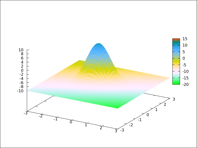
It also works with gray images.
(%i1) im: apply( 'matrix, makelist(makelist(random(200),i,1,30),i,1,30))$ (%i2) /* palette = color, default */ draw2d(image(im,0,0,30,30))$ (%i3) draw2d(palette = gray, image(im,0,0,30,30))$ (%i4) draw2d(palette = [15,20,-4], colorbox=false, image(im,0,0,30,30))$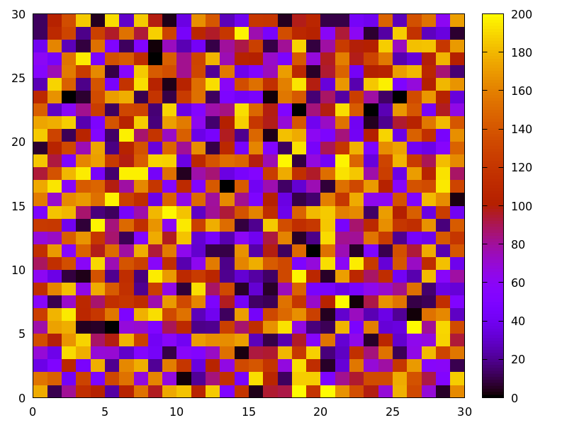
palettecan be a user defined lookup table. In this example, low values ofxare colored in red, and higher values in yellow.(%i1) draw3d( palette = [red, blue, yellow], enhanced3d = x, explicit(x^2+y^2,x,-1,1,y,-1,1)) $
See also
colorboxandenhanced3d.Categories: Package draw ·
- Graphic option: point_size 
Default value: 1
point_sizesets the size for plotted points. It must be a non negative number.This option has no effect when graphic option
point_typeis set todot.This option affects the following graphic objects:
Example:
(%i1) draw2d(points(makelist([random(20),random(50)],k,1,10)), point_size = 5, points(makelist(k,k,1,20),makelist(random(30),k,1,20)))$ Categories: Package draw ·
- Graphic option: point_type 
Default value: 1
point_typeindicates how isolated points are displayed; the value of this option can be any integer index greater or equal than -1, or the name of a point style:$none(-1),dot(0),plus(1),multiply(2),asterisk(3),square(4),filled_square(5),circle(6),filled_circle(7),up_triangle(8),filled_up_triangle(9),down_triangle(10),filled_down_triangle(11),diamant(12) andfilled_diamant(13).This option affects the following graphic objects:
Example:
(%i1) draw2d(xrange = [0,10], yrange = [0,10], point_size = 3, point_type = diamant, points([[1,1],[5,1],[9,1]]), point_type = filled_down_triangle, points([[1,2],[5,2],[9,2]]), point_type = asterisk, points([[1,3],[5,3],[9,3]]), point_type = filled_diamant, points([[1,4],[5,4],[9,4]]), point_type = 5, points([[1,5],[5,5],[9,5]]), point_type = 6, points([[1,6],[5,6],[9,6]]), point_type = filled_circle, points([[1,7],[5,7],[9,7]]), point_type = 8, points([[1,8],[5,8],[9,8]]), point_type = filled_diamant, points([[1,9],[5,9],[9,9]]) )$ Categories: Package draw ·
- Graphic option: points_joined 
Default value:
falseWhen
points_joinedistrue, points are joined by lines; whenfalse, isolated points are drawn. A third possible value for this graphic option isimpulses; in such case, vertical segments are drawn from points to the x-axis (2D) or to the xy-plane (3D).This option affects the following graphic objects:
Example:
(%i1) draw2d(xrange = [0,10], yrange = [0,4], point_size = 3, point_type = up_triangle, color = blue, points([[1,1],[5,1],[9,1]]), points_joined = true, point_type = square, line_type = dots, points([[1,2],[5,2],[9,2]]), point_type = circle, color = red, line_width = 7, points([[1,3],[5,3],[9,3]]) )$ Categories: Package draw ·
- Graphic option: proportional_axes 
Default value:
noneWhen
proportional_axesis equal toxyorxyz, the aspect ratio of the axis units will be set to 1:1 resulting in a 2D or 3D scene that will be drawn with axes proportional to their relative lengths.Since this is a global graphics option, its position in the scene description does not matter.
This option works with Gnuplot version 4.2.6 or greater.
Examples:
Single 2D plot.
(%i1) draw2d( ellipse(0,0,1,1,0,360), transparent=true, color = blue, line_width = 4, ellipse(0,0,2,1/2,0,360), proportional_axes = 'xy) $
Multiplot.
(%i1) draw( terminal = wxt, gr2d(proportional_axes = 'xy, explicit(x^2,x,0,1)), gr2d(explicit(x^2,x,0,1), xrange = [0,1], yrange = [0,2], proportional_axes='xy), gr2d(explicit(x^2,x,0,1)))$ Categories: Package draw ·
- Graphic option: surface_hide 
Default value:
falseIf
surface_hideistrue, hidden parts are not plotted in 3d surfaces.Since this is a global graphics option, its position in the scene description does not matter.
Example:
(%i1) draw(columns=2, gr3d(explicit(exp(sin(x)+cos(x^2)),x,-3,3,y,-3,3)), gr3d(surface_hide = true, explicit(exp(sin(x)+cos(x^2)),x,-3,3,y,-3,3)) )$ Categories: Package draw ·
- Graphic option: terminal 
Default value:
screenSelects the terminal to be used by Gnuplot; possible values are:
screen(default),png,pngcairo,jpg,gif,cairolatex_pdf,cairolatex_pdf_standalone,eps,eps_color,epslatex,epslatex_standalone,svg,canvas,dumb,dumb_file,pdf,pdfcairo,wxt,animated_gif,multipage_pdfcairo,multipage_pdf,multipage_eps,multipage_eps_color,tikz,tikz_standaloneandaquaterm.Terminals
screen,wxt,windowsandaquatermcan be also defined as a list with two elements: the name of the terminal itself and a non negative integer number. In this form, multiple windows can be opened at the same time, each with its corresponding number. This feature does not work in Windows platforms.Since this is a global graphics option, its position in the scene description does not matter. It can be also used as an argument of function
draw.N.B. pdfcairo requires Gnuplot 4.3 or newer.
pdfrequires Gnuplot to be compiled with the option--enable-pdfand libpdf must be installed. The pdf library is available from: http://www.pdflib.com/en/download/pdflib-family/pdflib-lite/Examples:
(%i1) /* screen terminal (default) */ draw2d(explicit(x^2,x,-1,1))$ (%i2) /* png file */ draw2d(terminal = 'png, explicit(x^2,x,-1,1))$ (%i3) /* jpg file */ draw2d(terminal = 'jpg, dimensions = [300,300], explicit(x^2,x,-1,1))$ (%i4) /* eps file */ draw2d(file_name = "myfile", explicit(x^2,x,-1,1), terminal = 'eps)$ (%i5) /* pdf file */ draw2d(file_name = "mypdf", dimensions = 100*[12.0,8.0], explicit(x^2,x,-1,1), terminal = 'pdf)$ (%i6) /* wxwidgets window */ draw2d(explicit(x^2,x,-1,1), terminal = 'wxt)$ (%i7) /* tikz file */ draw2d(explicit(x^2,x,-1,1), file_name = "mytikz", dimensions = [8,8], /* in cms */ terminal = 'tikz)$Multiple windows.
(%i1) draw2d(explicit(x^5,x,-2,2), terminal=[screen, 3])$ (%i2) draw2d(explicit(x^2,x,-2,2), terminal=[screen, 0])$
An animated gif file.
(%i1) draw( delay = 100, file_name = "zzz", terminal = 'animated_gif, gr2d(explicit(x^2,x,-1,1)), gr2d(explicit(x^3,x,-1,1)), gr2d(explicit(x^4,x,-1,1))); End of animation sequence (%o1) [gr2d(explicit), gr2d(explicit), gr2d(explicit)]Option
delayis only active in animated gif’s; it is ignored in any other case.Multipage output in eps format.
(%i1) draw( file_name = "parabol", terminal = multipage_eps, dimensions = 100*[10,10], gr2d(explicit(x^2,x,-1,1)), gr3d(explicit(x^2+y^2,x,-1,1,y,-1,1))) $See also
file_name,dimensions_drawanddelay.Categories: Package draw ·
- Graphic option: title 
Default value:
""(empty string)Option
title, a string, is the main title for the scene. By default, no title is written.Since this is a global graphics option, its position in the scene description does not matter.
Example:
(%i1) draw2d(explicit(exp(u),u,-2,2), title = "Exponential function")$ Categories: Package draw ·
- Graphic option: transform 
Default value:
noneIf
transformisnone, the space is not transformed and graphic objects are drawn as defined. When a space transformation is desired, a list must be assigned to optiontransform. In case of a 2D scene, the list takes the form[f1(x,y), f2(x,y), x, y]. In case of a 3D scene, the list is of the form[f1(x,y,z), f2(x,y,z), f3(x,y,z), x, y, z].The names of the variables defined in the lists may be different to those used in the definitions of the graphic objects.
Examples:
Rotation in 2D.
(%i1) th : %pi / 4$ (%i2) draw2d( color = "#e245f0", proportional_axes = 'xy, line_width = 8, triangle([3,2],[7,2],[5,5]), border = false, fill_color = yellow, transform = [cos(th)*x - sin(th)*y, sin(th)*x + cos(th)*y, x, y], triangle([3,2],[7,2],[5,5]) )$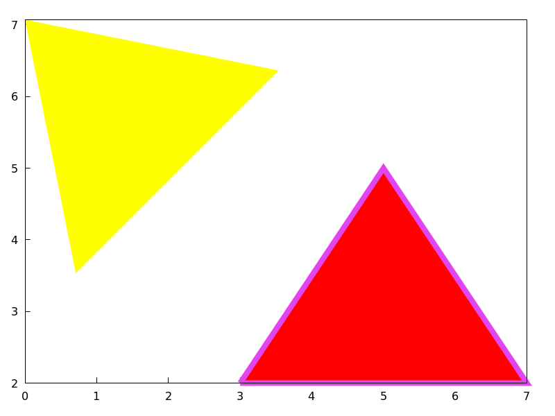
Translation in 3D.
(%i1) draw3d( color = "#a02c00", explicit(20*exp(-x^2-y^2)-10,x,-3,3,y,-3,3), transform = [x+10,y+10,z+10,x,y,z], color = blue, explicit(20*exp(-x^2-y^2)-10,x,-3,3,y,-3,3) )$Categories: Package draw ·
- Graphic option: transparent 
Default value:
falseIf
transparentisfalse, interior regions of polygons are filled according tofill_color.This option affects the following graphic objects:
Example:
(%i1) draw2d(polygon([[3,2],[7,2],[5,5]]), transparent = true, color = blue, polygon([[5,2],[9,2],[7,5]]) )$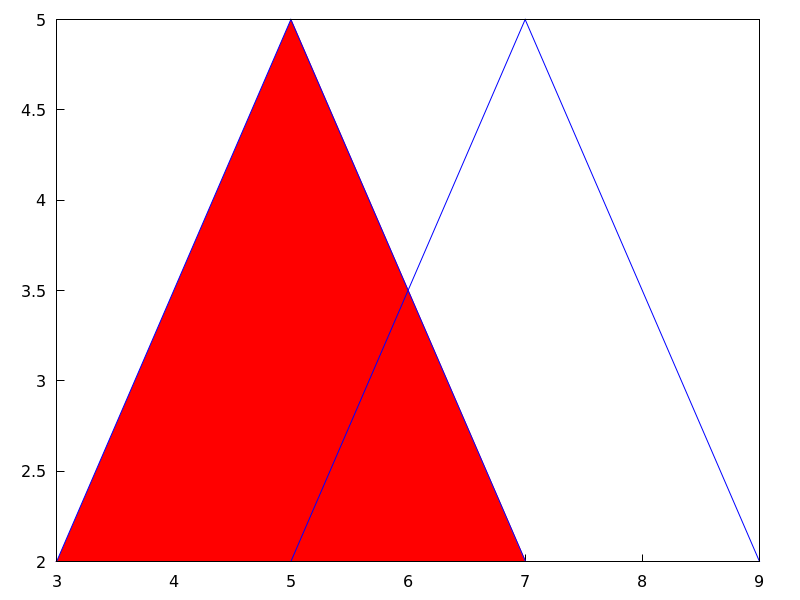 Categories: Package draw ·
- Graphic option: unit_vectors 
Default value:
falseIf
unit_vectorsistrue, vectors are plotted with module 1. This is useful for plotting vector fields. Ifunit_vectorsisfalse, vectors are plotted with its original length.This option is relevant only for
vectorobjects.Example:
(%i1) draw2d(xrange = [-1,6], yrange = [-1,6], head_length = 0.1, vector([0,0],[5,2]), unit_vectors = true, color = red, vector([0,3],[5,2]))$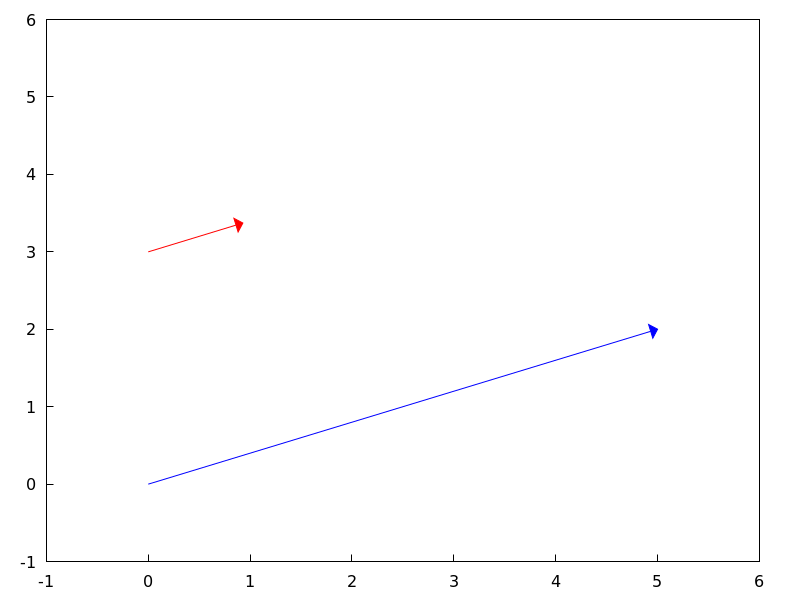 Categories: Package draw ·
- Graphic option: user_preamble 
Default value:
""(empty string)Expert Gnuplot users can make use of this option to fine tune Gnuplot’s behaviour by writing settings to be sent before the
plotorsplotcommand.The value of this option must be a string or a list of strings (one per line).
Since this is a global graphics option, its position in the scene description does not matter.
Example:
Tell Gnuplot to draw axes and grid on top of graphics objects,
(%i1) draw2d( xaxis =true, xaxis_type=solid, yaxis =true, yaxis_type=solid, user_preamble="set grid front", region(x^2+y^2<1 ,x,-1.5,1.5,y,-1.5,1.5))$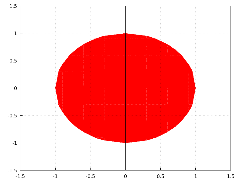
Tell gnuplot to draw all contour lines in black
(%i1) draw3d( contour=both, surface_hide=true,enhanced3d=true,wired_surface=true, contour_levels=10, user_preamble="set for [i=1:8] linetype i dashtype i linecolor 0", explicit(sin(x)*cos(y),x,1,10,y,1,10) );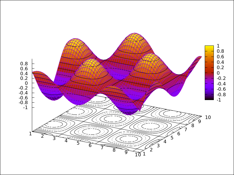 Categories: Package draw ·
- Graphic option: view 
Default value:
[60,30]A pair of angles, measured in degrees, indicating the view direction in a 3D scene. The first angle is the vertical rotation around the x axis, in the range [0, 360]. The second one is the horizontal rotation around the z axis, in the range [0, 360].
If option
viewis given the valuemap, the view direction is set to be perpendicular to the xy-plane.Since this is a global graphics option, its position in the scene description does not matter.
Example:
(%i1) draw3d(view = [170, 50], enhanced3d = true, explicit(sin(x^2+y^2),x,-2,2,y,-2,2) )$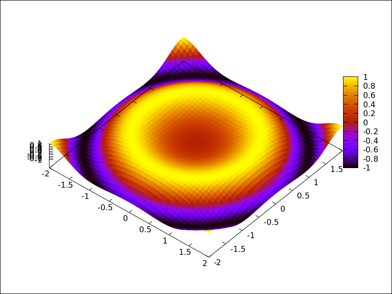
(%i2) draw3d(view = map, enhanced3d = true, explicit(sin(x^2+y^2),x,-2,2,y,-2,2) )$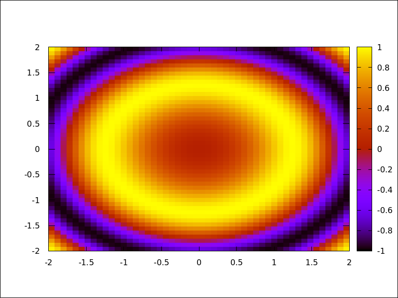 Categories: Package draw ·
- Graphic option: wired_surface 
Default value:
falseIndicates whether 3D surfaces in
enhanced3dmode show the grid joining the points or not.Since this is a global graphics option, its position in the scene description does not matter.
Example:
(%i1) draw3d( enhanced3d = [sin(x),x,y], wired_surface = true, explicit(x^2+y^2,x,-1,1,y,-1,1)) $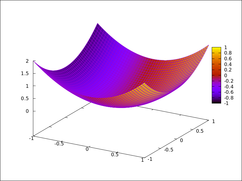 Categories: Package draw ·
- Graphic option: x_voxel 
Default value: 10
x_voxelis the number of voxels in the x direction to be used by the marching cubes algorithm implemented by the 3dimplicitobject. It is also used by graphic objectregion.Categories: Package draw ·
- Graphic option: xaxis 
Default value:
falseIf
xaxisistrue, the x axis is drawn.Since this is a global graphics option, its position in the scene description does not matter.
Example:
(%i1) draw2d(explicit(x^3,x,-1,1), xaxis = true, xaxis_color = blue)$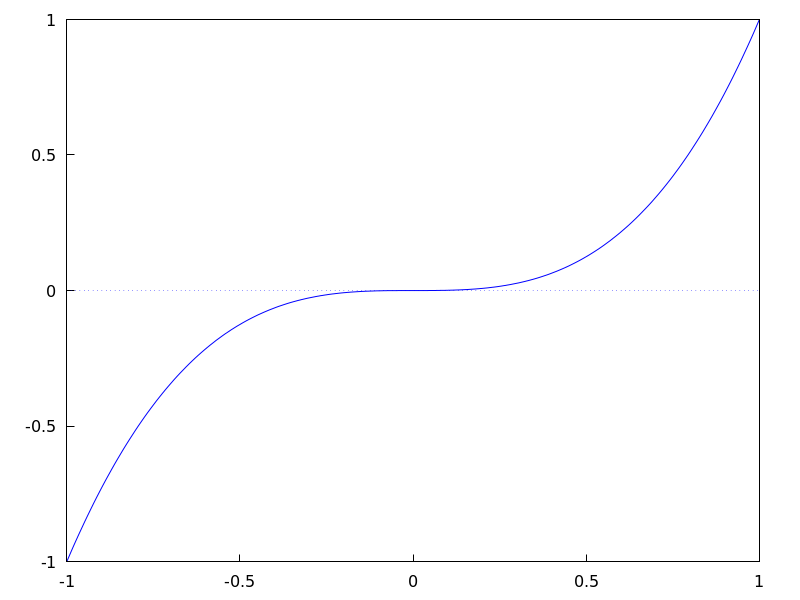
See also
xaxis_width,xaxis_typeandxaxis_color.Categories: Package draw ·
- Graphic option: xaxis_color 
Default value:
"black"xaxis_colorspecifies the color for the x axis. Seecolorto know how colors are defined.Since this is a global graphics option, its position in the scene description does not matter.
Example:
(%i1) draw2d(explicit(x^3,x,-1,1), xaxis = true, xaxis_color = red)$See also
xaxis,xaxis_widthandxaxis_type.Categories: Package draw ·
- Graphic option: xaxis_secondary 
Default value:
falseIf
xaxis_secondaryistrue, function values can be plotted with respect to the second x axis, which will be drawn on top of the scene.Note that this is a local graphics option which only affects to 2d plots.
Example:
(%i1) draw2d( key = "Bottom x-axis", explicit(x+1,x,1,2), color = red, key = "Above x-axis", xtics_secondary = true, xaxis_secondary = true, explicit(x^2,x,-1,1)) $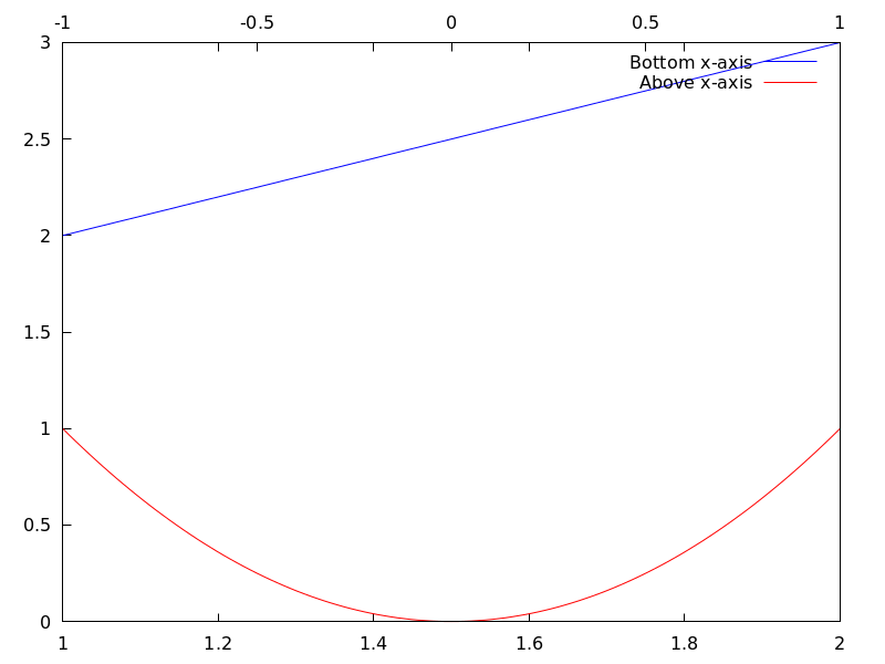
See also
xrange_secondary,xtics_secondary,xtics_rotate_secondary,xtics_axis_secondaryandxaxis_secondary.Categories: Package draw ·
- Graphic option: xaxis_type 
Default value:
dotsxaxis_typeindicates how the x axis is displayed; possible values aresolidanddotsSince this is a global graphics option, its position in the scene description does not matter.
Example:
(%i1) draw2d(explicit(x^3,x,-1,1), xaxis = true, xaxis_type = solid)$See also
xaxis,xaxis_widthandxaxis_color.Categories: Package draw ·
- Graphic option: xaxis_width 
Default value: 1
xaxis_widthis the width of the x axis. Its value must be a positive number.Since this is a global graphics option, its position in the scene description does not matter.
Example:
(%i1) draw2d(explicit(x^3,x,-1,1), xaxis = true, xaxis_width = 3)$See also
xaxis,xaxis_typeandxaxis_color.Categories: Package draw ·
- Graphic option: xlabel 
Default value:
""Option
xlabel, a string, is the label for the x axis. By default, the axis is labeled with string"x".Since this is a global graphics option, its position in the scene description does not matter.
Example:
(%i1) draw2d(xlabel = "Time", explicit(exp(u),u,-2,2), ylabel = "Population")$See also
xlabel_secondary,ylabel,ylabel_secondaryandzlabel_draw.Categories: Package draw ·
- Graphic option: xlabel_secondary 
Default value:
""(empty string)Option
xlabel_secondary, a string, is the label for the secondary x axis. By default, no label is written.Since this is a global graphics option, its position in the scene description does not matter.
Example:
(%i1) draw2d( xaxis_secondary=true,yaxis_secondary=true, xtics_secondary=true,ytics_secondary=true, xlabel_secondary="t[s]", ylabel_secondary="U[V]", explicit(sin(t),t,0,10) )$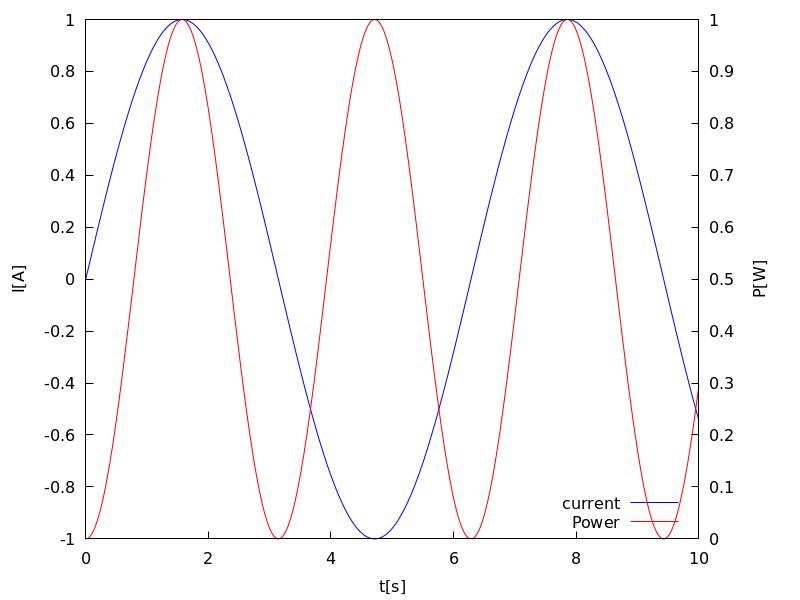
See also
xlabel_draw,ylabel_draw,ylabel_secondaryandzlabel_draw.Categories: Package draw ·
- Graphic option: xrange 
Default value:
autoIf
xrangeisauto, the range for the x coordinate is computed automatically.If the user wants a specific interval for x, it must be given as a Maxima list, as in
xrange=[-2, 3].Since this is a global graphics option, its position in the scene description does not matter.
Example:
(%i1) draw2d(xrange = [-3,5], explicit(x^2,x,-1,1))$Categories: Package draw ·
- Graphic option: xrange_secondary 
Default value:
autoIf
xrange_secondaryisauto, the range for the second x axis is computed automatically.If the user wants a specific interval for the second x axis, it must be given as a Maxima list, as in
xrange_secondary=[-2, 3].Since this is a global graphics option, its position in the scene description does not matter.
See also
xrange,yrange,zrangeandyrange_secondary.Categories: Package draw ·
- Graphic option: xtics 
Default value:
trueThis graphic option controls the way tic marks are drawn on the x axis.
- When option
xticsis bounded to symbol true, tic marks are drawn automatically. - When option
xticsis bounded to symbol false, tic marks are not drawn. - When option
xticsis bounded to a positive number, this is the distance between two consecutive tic marks. - When option
xticsis bounded to a list of length three of the form[start,incr,end], tic marks are plotted fromstarttoendat intervals of lengthincr. - When option
xticsis bounded to a set of numbers of the form{n1, n2, ...}, tic marks are plotted at valuesn1,n2, ... - When option
xticsis bounded to a set of pairs of the form{["label1", n1], ["label2", n2], ...}, tic marks corresponding to valuesn1,n2, ... are labeled with"label1","label2", ..., respectively.
Since this is a global graphics option, its position in the scene description does not matter.
Examples:
Disable tics.
(%i1) draw2d(xtics = 'false, explicit(x^3,x,-1,1) )$Tics every 1/4 units.
(%i1) draw2d(xtics = 1/4, explicit(x^3,x,-1,1) )$Tics from -3/4 to 3/4 in steps of 1/8.
(%i1) draw2d(xtics = [-3/4,1/8,3/4], explicit(x^3,x,-1,1) )$Tics at points -1/2, -1/4 and 3/4.
(%i1) draw2d(xtics = {-1/2,-1/4,3/4}, explicit(x^3,x,-1,1) )$Labeled tics.
(%i1) draw2d(xtics = {["High",0.75],["Medium",0],["Low",-0.75]}, explicit(x^3,x,-1,1) )$See also
ytics_draw, andztics_draw.Categories: Package draw ·- When option
- Graphic option: xtics_axis 
Default value:
falseIf
xtics_axisistrue, tic marks and their labels are plotted just along the x axis, if it isfalsetics are plotted on the border.Since this is a global graphics option, its position in the scene description does not matter.
Categories: Package draw ·
- Graphic option: xtics_rotate 
Default value:
falseIf
xtics_rotateistrue, tic marks on the x axis are rotated 90 degrees.Since this is a global graphics option, its position in the scene description does not matter.
Categories: Package draw ·
- Graphic option: xtics_rotate_secondary 
Default value:
falseIf
xtics_rotate_secondaryistrue, tic marks on the secondary x axis are rotated 90 degrees.Since this is a global graphics option, its position in the scene description does not matter.
Categories: Package draw ·
- Graphic option: xtics_secondary 
Default value:
autoThis graphic option controls the way tic marks are drawn on the second x axis.
See
xtics_drawfor a complete description.Categories: Package draw ·
- Graphic option: xtics_secondary_axis 
Default value:
falseIf
xtics_secondary_axisistrue, tic marks and their labels are plotted just along the secondary x axis, if it isfalsetics are plotted on the border.Since this is a global graphics option, its position in the scene description does not matter.
Categories: Package draw ·
- Graphic option: xu_grid 
Default value: 30
xu_gridis the number of coordinates of the first variable (xin explicit anduin parametric 3d surfaces) to build the grid of sample points.This option affects the following graphic objects:
-
gr3d:explicitandparametric_surface.
Example:
(%i1) draw3d(xu_grid = 10, yv_grid = 50, explicit(x^2+y^2,x,-3,3,y,-3,3) )$See also
yv_grid.Categories: Package draw ·-
- Graphic option: xy_file 
Default value:
""(empty string)xy_fileis the name of the file where the coordinates will be saved after clicking with the mouse button and hitting the ’x’ key. By default, no coordinates are saved.Since this is a global graphics option, its position in the scene description does not matter.
Categories: Package draw ·
- Graphic option: xyplane 
Default value:
falseAllocates the xy-plane in 3D scenes. When
xyplaneisfalse, the xy-plane is placed automatically; when it is a real number, the xy-plane intersects the z-axis at this level. This option has no effect in 2D scenes.Since this is a global graphics option, its position in the scene description does not matter.
Example:
(%i1) draw3d(xyplane = %e-2, explicit(x^2+y^2,x,-1,1,y,-1,1))$Categories: Package draw ·
- Graphic option: y_voxel 
Default value: 10
y_voxelis the number of voxels in the y direction to be used by the marching cubes algorithm implemented by the 3dimplicitobject. It is also used by graphic objectregion.Categories: Package draw ·
- Graphic option: yaxis 
Default value:
falseIf
yaxisistrue, the y axis is drawn.Since this is a global graphics option, its position in the scene description does not matter.
Example:
(%i1) draw2d(explicit(x^3,x,-1,1), yaxis = true, yaxis_color = blue)$See also
yaxis_width,yaxis_typeandyaxis_color.Categories: Package draw ·
- Graphic option: yaxis_color 
Default value:
"black"yaxis_colorspecifies the color for the y axis. Seecolorto know how colors are defined.Since this is a global graphics option, its position in the scene description does not matter.
Example:
(%i1) draw2d(explicit(x^3,x,-1,1), yaxis = true, yaxis_color = red)$See also
yaxis,yaxis_widthandyaxis_type.Categories: Package draw ·
- Graphic option: yaxis_secondary 
Default value:
falseIf
yaxis_secondaryistrue, function values can be plotted with respect to the second y axis, which will be drawn on the right side of the scene.Note that this is a local graphics option which only affects to 2d plots.
Example:
(%i1) draw2d( explicit(sin(x),x,0,10), yaxis_secondary = true, ytics_secondary = true, color = blue, explicit(100*sin(x+0.1)+2,x,0,10));See also
yrange_secondary,ytics_secondary,ytics_rotate_secondaryandytics_axis_secondaryCategories: Package draw ·
- Graphic option: yaxis_type 
Default value:
dotsyaxis_typeindicates how the y axis is displayed; possible values aresolidanddots.Since this is a global graphics option, its position in the scene description does not matter.
Example:
(%i1) draw2d(explicit(x^3,x,-1,1), yaxis = true, yaxis_type = solid)$See also
yaxis,yaxis_widthandyaxis_color.Categories: Package draw ·
- Graphic option: yaxis_width 
Default value: 1
yaxis_widthis the width of the y axis. Its value must be a positive number.Since this is a global graphics option, its position in the scene description does not matter.
Example:
(%i1) draw2d(explicit(x^3,x,-1,1), yaxis = true, yaxis_width = 3)$See also
yaxis,yaxis_typeandyaxis_color.Categories: Package draw ·
- Graphic option: ylabel 
Default value:
""Option
ylabel, a string, is the label for the y axis. By default, the axis is labeled with string"y".Since this is a global graphics option, its position in the scene description does not matter.
Example:
(%i1) draw2d(xlabel = "Time", ylabel = "Population", explicit(exp(u),u,-2,2) )$See also
xlabel_draw,xlabel_secondary,ylabel_secondary, andzlabel_draw.Categories: Package draw ·
- Graphic option: ylabel_secondary 
Default value:
""(empty string)Option
ylabel_secondary, a string, is the label for the secondary y axis. By default, no label is written.Since this is a global graphics option, its position in the scene description does not matter.
Example:
(%i1) draw2d( key_pos=bottom_right, key="current", xlabel="t[s]", ylabel="I[A]",ylabel_secondary="P[W]", explicit(sin(t),t,0,10), yaxis_secondary=true, ytics_secondary=true, color=red,key="Power", explicit((sin(t))^2,t,0,10) )$See also
xlabel_draw,xlabel_secondary,ylabel_drawandzlabel_draw.Categories: Package draw ·
- Graphic option: yrange 
Default value:
autoIf
yrangeisauto, the range for the y coordinate is computed automatically.If the user wants a specific interval for y, it must be given as a Maxima list, as in
yrange=[-2, 3].Since this is a global graphics option, its position in the scene description does not matter.
Example:
(%i1) draw2d(yrange = [-2,3], explicit(x^2,x,-1,1), xrange = [-3,3])$See also
xrange,yrange_secondaryandzrange.Categories: Package draw ·
- Graphic option: yrange_secondary 
Default value:
autoIf
yrange_secondaryisauto, the range for the second y axis is computed automatically.If the user wants a specific interval for the second y axis, it must be given as a Maxima list, as in
yrange_secondary=[-2, 3].Since this is a global graphics option, its position in the scene description does not matter.
Example:
(%i1) draw2d( explicit(sin(x),x,0,10), yaxis_secondary = true, ytics_secondary = true, yrange = [-3, 3], yrange_secondary = [-20, 20], color = blue, explicit(100*sin(x+0.1)+2,x,0,10)) $See also
xrange,yrangeandzrange.Categories: Package draw ·
- Graphic option: ytics 
Default value:
trueThis graphic option controls the way tic marks are drawn on the y axis.
See
xticsfor a complete description.Categories: Package draw ·
- Graphic option: ytics_axis 
Default value:
falseIf
ytics_axisistrue, tic marks and their labels are plotted just along the y axis, if it isfalsetics are plotted on the border.Since this is a global graphics option, its position in the scene description does not matter.
Categories: Package draw ·
- Graphic option: ytics_rotate 
Default value:
falseIf
ytics_rotateistrue, tic marks on the y axis are rotated 90 degrees.Since this is a global graphics option, its position in the scene description does not matter.
Categories: Package draw ·
- Graphic option: ytics_rotate_secondary 
Default value:
falseIf
ytics_rotate_secondaryistrue, tic marks on the secondary y axis are rotated 90 degrees.Since this is a global graphics option, its position in the scene description does not matter.
Categories: Package draw ·
- Graphic option: ytics_secondary 
Default value:
autoThis graphic option controls the way tic marks are drawn on the second y axis.
See
xticsfor a complete description.Categories: Package draw ·
- Graphic option: ytics_secondary_axis 
Default value:
falseIf
ytics_secondary_axisistrue, tic marks and their labels are plotted just along the secondary y axis, if it isfalsetics are plotted on the border.Since this is a global graphics option, its position in the scene description does not matter.
Categories: Package draw ·
- Graphic option: yv_grid 
Default value: 30
yv_gridis the number of coordinates of the second variable (yin explicit andvin parametric 3d surfaces) to build the grid of sample points.This option affects the following graphic objects:
-
gr3d:explicitandparametric_surface.
Example:
(%i1) draw3d(xu_grid = 10, yv_grid = 50, explicit(x^2+y^2,x,-3,3,y,-3,3) )$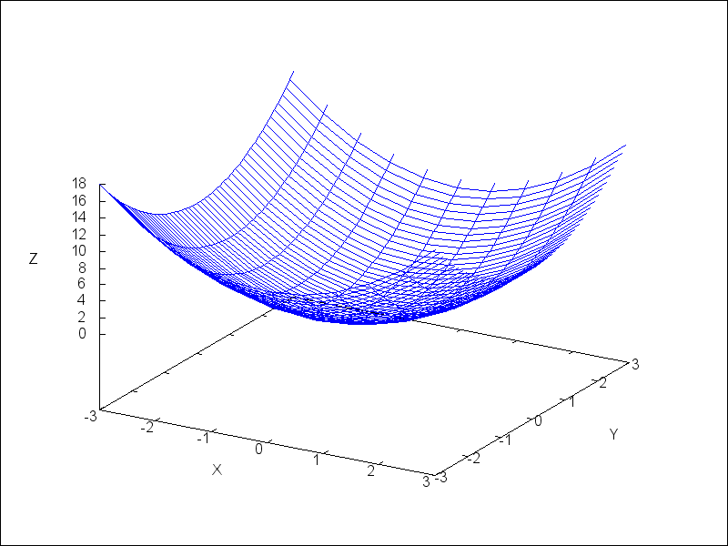
See also
xu_grid.Categories: Package draw ·-
- Graphic option: z_voxel 
Default value: 10
z_voxelis the number of voxels in the z direction to be used by the marching cubes algorithm implemented by the 3dimplicitobject.Categories: Package draw ·
- Graphic option: zaxis 
Default value:
falseIf
zaxisistrue, the z axis is drawn in 3D plots. This option has no effect in 2D scenes.Since this is a global graphics option, its position in the scene description does not matter.
Example:
(%i1) draw3d(explicit(x^2+y^2,x,-1,1,y,-1,1), zaxis = true, zaxis_type = solid, zaxis_color = blue)$See also
zaxis_width,zaxis_typeandzaxis_color.Categories: Package draw ·
- Graphic option: zaxis_color 
Default value:
"black"zaxis_colorspecifies the color for the z axis. Seecolorto know how colors are defined. This option has no effect in 2D scenes.Since this is a global graphics option, its position in the scene description does not matter.
Example:
(%i1) draw3d(explicit(x^2+y^2,x,-1,1,y,-1,1), zaxis = true, zaxis_type = solid, zaxis_color = red)$See also
zaxis,zaxis_widthandzaxis_type.Categories: Package draw ·
- Graphic option: zaxis_type 
Default value:
dotszaxis_typeindicates how the z axis is displayed; possible values aresolidanddots. This option has no effect in 2D scenes.Since this is a global graphics option, its position in the scene description does not matter.
Example:
(%i1) draw3d(explicit(x^2+y^2,x,-1,1,y,-1,1), zaxis = true, zaxis_type = solid)$See also
zaxis,zaxis_widthandzaxis_color.Categories: Package draw ·
- Graphic option: zaxis_width 
Default value: 1
zaxis_widthis the width of the z axis. Its value must be a positive number. This option has no effect in 2D scenes.Since this is a global graphics option, its position in the scene description does not matter.
Example:
(%i1) draw3d(explicit(x^2+y^2,x,-1,1,y,-1,1), zaxis = true, zaxis_type = solid, zaxis_width = 3)$See also
zaxis,zaxis_typeandzaxis_color.Categories: Package draw ·
- Graphic option: zlabel 
Default value:
""Option
zlabel, a string, is the label for the z axis. By default, the axis is labeled with string"z".Since this is a global graphics option, its position in the scene description does not matter.
Example:
(%i1) draw3d(zlabel = "Z variable", ylabel = "Y variable", explicit(sin(x^2+y^2),x,-2,2,y,-2,2), xlabel = "X variable" )$See also
xlabel_draw,ylabel_draw, andzlabel_rotate.Categories: Package draw ·
- Graphic option: zlabel_rotate 
Default value:
"auto"This graphics option allows to choose if the z axis label of 3d plots is drawn horizontal (
false), vertical (true) or if maxima automatically chooses an orientation based on the length of the label (auto).Since this is a global graphics option, its position in the scene description does not matter.
Example:
(%i1) draw3d( explicit(sin(x)*sin(y),x,0,10,y,0,10), zlabel_rotate=false )$See also
zlabel_draw.Categories: Package draw ·
- Graphic option: zrange 
Default value:
autoIf
zrangeisauto, the range for the z coordinate is computed automatically.If the user wants a specific interval for z, it must be given as a Maxima list, as in
zrange=[-2, 3].Since this is a global graphics option, its position in the scene description does not matter.
Example:
(%i1) draw3d(yrange = [-3,3], zrange = [-2,5], explicit(x^2+y^2,x,-1,1,y,-1,1), xrange = [-3,3])$Categories: Package draw ·
- Graphic option: ztics 
Default value:
trueThis graphic option controls the way tic marks are drawn on the z axis.
See
xtics_drawfor a complete description.Categories: Package draw ·
- Graphic option: ztics_axis 
Default value:
falseIf
ztics_axisistrue, tic marks and their labels are plotted just along the z axis, if it isfalsetics are plotted on the border.Since this is a global graphics option, its position in the scene description does not matter.
Categories: Package draw ·
- Graphic option: ztics_rotate 
Default value:
falseIf
ztics_rotateistrue, tic marks on the z axis are rotated 90 degrees.Since this is a global graphics option, its position in the scene description does not matter.
Categories: Package draw ·
55.2.4 Graphics objects
- Graphic object: bars ([x1,h1,w1], [x2,h2,w2, ...]) 
Draws vertical bars in 2D.
2D
bars ([x1,h1,w1], [x2,h2,w2, ...])draws bars centered at values x1, x2, ... with heights h1, h2, ... and widths w1, w2, ...This object is affected by the following graphic options:
key,fill_color,fill_densityandline_width.Example:
(%i1) draw2d( key = "Group A", fill_color = blue, fill_density = 0.2, bars([0.8,5,0.4],[1.8,7,0.4],[2.8,-4,0.4]), key = "Group B", fill_color = red, fill_density = 0.6, line_width = 4, bars([1.2,4,0.4],[2.2,-2,0.4],[3.2,5,0.4]), xaxis = true); Categories: Package draw ·
- Graphic object: cylindrical (radius, z, minz, maxz, azi, minazi, maxazi) 
Draws 3D functions defined in cylindrical coordinates.
3D
cylindrical(radius, z, minz, maxz, azi, minazi, maxazi)plots the functionradius(z, azi)defined in cylindrical coordinates, with variable z taking values from minz to maxz and azimuth azi taking values from minazi to maxazi.This object is affected by the following graphic options:
xu_grid,yv_grid,line_type,key,wired_surface,enhanced3dandcolorExample:
(%i1) draw3d(cylindrical(1,z,-2,2,az,0,2*%pi))$
 Categories: Package draw ·
- Graphic object: elevation_grid (mat,x0,y0,width,height) 
Draws matrix mat in 3D space. z values are taken from mat, the abscissas range from x0 to x0 + width and ordinates from y0 to y0 + height. Element a(1,1) is projected on point (x0,y0+height), a(1,n) on (x0+width,y0+height), a(m,1) on (x0,y0), and a(m,n) on (x0+width,y0).
This object is affected by the following graphic options:
line_type,,line_widthkey,wired_surface,enhanced3dandcolorIn older versions of Maxima,
elevation_gridwas calledmesh. See alsomesh.Example:
(%i1) m: apply( matrix, makelist(makelist(random(10.0),k,1,30),i,1,20)) $ (%i2) draw3d( color = blue, elevation_grid(m,0,0,3,2), xlabel = "x", ylabel = "y", surface_hide = true); Categories: Package draw ·
- Graphic object: ellipse (xc, yc, a, b, ang1, ang2) 
Draws ellipses and circles in 2D.
2D
ellipse (xc, yc, a, b, ang1, ang2)plots an ellipse centered at[xc, yc]with horizontal and vertical semi axis a and b, respectively, starting at angle ang1 with an amplitude equal to angle ang2.This object is affected by the following graphic options:
nticks,transparent,fill_color,fill_density,border,line_width,line_type,keyandcolorExample:
(%i1) draw2d(transparent = false, fill_color = red, color = gray30, transparent = false, line_width = 5, ellipse(0,6,3,2,270,-270), /* center (x,y), a, b, start & end in degrees */ transparent = true, color = blue, line_width = 3, ellipse(2.5,6,2,3,30,-90), xrange = [-3,6], yrange = [2,9] )$ Categories: Package draw ·
- Graphic object: errors ([x1, x2, …], [y1, y2, …]) 
Draws points with error bars, horizontally, vertically or both, depending on the value of option
error_type.2D
If
error_type = x, arguments toerrorsmust be of the form[x, y, xdelta]or[x, y, xlow, xhigh]. Iferror_type = y, arguments must be of the form[x, y, ydelta]or[x, y, ylow, yhigh]. Iferror_type = xyorerror_type = boxes, arguments toerrorsmust be of the form[x, y, xdelta, ydelta]or[x, y, xlow, xhigh, ylow, yhigh].See also
error_type.This object is affected by the following graphic options:
error_type,points_joined,line_width,key,line_type,colorfill_density,xaxis_secondaryandyaxis_secondary.Option
fill_densityis only relevant whenerror_type=boxes.Examples:
Horizontal error bars.
(%i1) draw2d( error_type = 'y, errors([[1,2,1], [3,5,3], [10,3,1], [17,6,2]]))$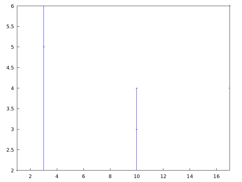
Vertical and horizontal error bars.
(%i1) draw2d( error_type = 'xy, points_joined = true, color = blue, errors([[1,2,1,2], [3,5,2,1], [10,3,1,1], [17,6,1/2,2]]));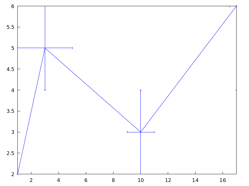 Categories: Package draw ·
- Graphic object: explicit
explicit (expr,var,minval,maxval)
explicit (fcn,var,minval,maxval)
explicit (expr,var1,minval1,maxval1,var2,minval2,maxval2)
explicit (fcn,var1,minval1,maxval1,var2,minval2,maxval2) ¶ -
Draws explicit functions in 2D and 3D.
2D
explicit(fcn,var,minval,maxval)plots explicit function fcn, with variable var taking values from minval to maxval.This object is affected by the following graphic options:
nticks,adapt_depth,draw_realpart,line_width,line_type,key,filled_func,fill_color,fill_density, andcolorExample:
(%i1) draw2d(line_width = 3, color = blue, explicit(x^2,x,-3,3) )$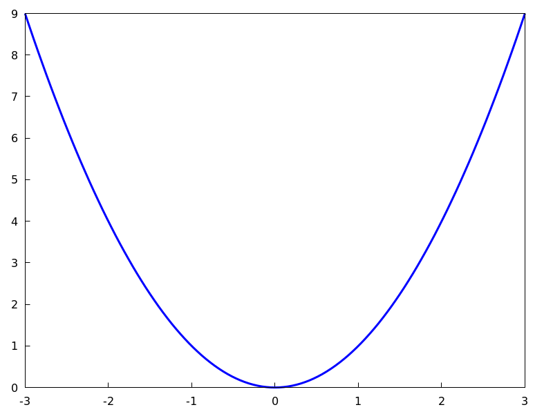
(%i2) draw2d(fill_color = brown, filled_func = true, explicit(x^2,x,-3,3) )$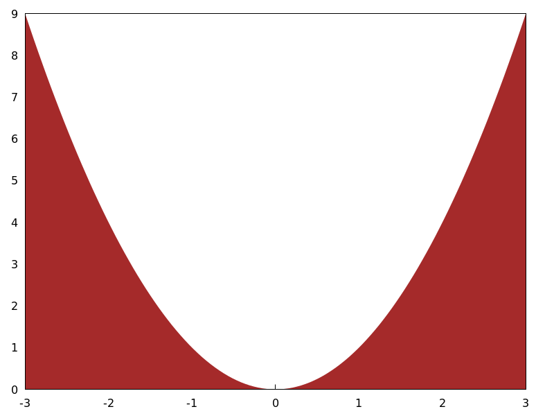
3D
explicit(fcn, var1, minval1, maxval1, var2, minval2, maxval2)plots the explicit function fcn, with variable var1 taking values from minval1 to maxval1 and variable var2 taking values from minval2 to maxval2.This object is affected by the following graphic options:
draw_realpart,xu_grid,yv_grid,line_type,line_width,key,wired_surface,enhanced3dandcolor.Example:
(%i1) draw3d(key = "Gauss", color = "#a02c00", explicit(20*exp(-x^2-y^2)-10,x,-3,3,y,-3,3), yv_grid = 10, color = blue, key = "Plane", explicit(x+y,x,-5,5,y,-5,5), surface_hide = true)$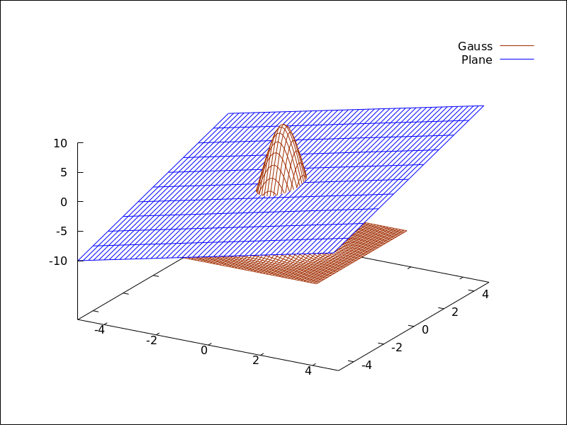
See also
filled_funcfor filled functions.Categories: Package draw ·
- Graphic object: image (im,x0,y0,width,height) 
Renders images in 2D.
2D
image (im,x0,y0,width,height)plots image im in the rectangular region from vertex(x0,y0)to(x0+width,y0+height)on the real plane. Argument im must be a matrix of real numbers, a matrix of vectors of length three or a picture object.If im is a matrix of real numbers or a levels picture object, pixel values are interpreted according to graphic option
palette, which is a vector of length three with components ranging from -36 to +36; each value is an index for a formula mapping the levels onto red, green and blue colors, respectively:0: 0 1: 0.5 2: 1 3: x 4: x^2 5: x^3 6: x^4 7: sqrt(x) 8: sqrt(sqrt(x)) 9: sin(90x) 10: cos(90x) 11: |x-0.5| 12: (2x-1)^2 13: sin(180x) 14: |cos(180x)| 15: sin(360x) 16: cos(360x) 17: |sin(360x)| 18: |cos(360x)| 19: |sin(720x)| 20: |cos(720x)| 21: 3x 22: 3x-1 23: 3x-2 24: |3x-1| 25: |3x-2| 26: (3x-1)/2 27: (3x-2)/2 28: |(3x-1)/2| 29: |(3x-2)/2| 30: x/0.32-0.78125 31: 2*x-0.84 32: 4x;1;-2x+1.84;x/0.08-11.5 33: |2*x - 0.5| 34: 2*x 35: 2*x - 0.5 36: 2*x - 1
negative numbers mean negative colour component.
palette = grayandpalette = colorare short cuts forpalette = [3,3,3]andpalette = [7,5,15], respectively.If im is a matrix of vectors of length three or an rgb picture object, they are interpreted as red, green and blue color components.
Examples:
If im is a matrix of real numbers, pixel values are interpreted according to graphic option
palette.(%i1) im: apply( 'matrix, makelist(makelist(random(200),i,1,30),i,1,30))$ (%i2) /* palette = color, default */ draw2d(image(im,0,0,30,30))$
(%i3) draw2d(palette = gray, image(im,0,0,30,30))$

(%i4) draw2d(palette = [15,20,-4], colorbox=false, image(im,0,0,30,30))$
See also
colorbox.If im is a matrix of vectors of length three, they are interpreted as red, green and blue color components.
(%i1) im: apply( 'matrix, makelist( makelist([random(300), random(300), random(300)],i,1,30),i,1,30))$ (%i2) draw2d(image(im,0,0,30,30))$
Package
drawautomatically loads packagepicture. In this example, a level picture object is built by hand and then rendered.(%i1) im: make_level_picture([45,87,2,134,204,16],3,2); (%o1) picture(level, 3, 2, {Array: #(45 87 2 134 204 16)}) (%i2) /* default color palette */ draw2d(image(im,0,0,30,30))$
(%i3) /* gray palette */ draw2d(palette = gray, image(im,0,0,30,30))$
An xpm file is read and then rendered.
(%i1) im: read_xpm("myfile.xpm")$ (%i2) draw2d(image(im,0,0,10,7))$See also
make_level_picture,make_rgb_pictureandread_xpm.http://www.telefonica.net/web2/biomates/maxima/gpdraw/image
contains more elaborated examples.Categories: Package draw ·
- Graphic object: implicit
implicit (fcn,x,xmin,xmax,y,ymin,ymax)
implicit (fcn,x,xmin,xmax,y,ymin,ymax,z,zmin,zmax) ¶ -
Draws implicit functions in 2D and 3D.
2D
implicit(fcn,x,xmin,xmax,y,ymin,ymax)plots the implicit function defined by fcn, with variable x taking values from xmin to xmax, and variable y taking values from ymin to ymax.This object is affected by the following graphic options:
ip_grid,ip_grid_in,line_width,line_type,keyandcolor.Example:
(%i1) draw2d(grid = true, line_type = solid, key = "y^2=x^3-2*x+1", implicit(y^2=x^3-2*x+1, x, -4,4, y, -4,4), line_type = dots, key = "x^3+y^3 = 3*x*y^2-x-1", implicit(x^3+y^3 = 3*x*y^2-x-1, x,-4,4, y,-4,4), title = "Two implicit functions" )$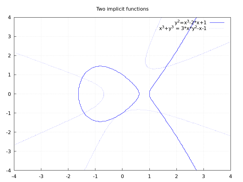
3D
implicit (fcn,x,xmin,xmax, y,ymin,ymax, z,zmin,zmax)plots the implicit surface defined by fcn, with variable x taking values from xmin to xmax, variable y taking values from ymin to ymax and variable z taking values from zmin to zmax. This object implements the marching cubes algorithm.This object is affected by the following graphic options:
x_voxel,y_voxel,z_voxel,line_width,line_type,key,wired_surface,enhanced3dandcolor.Example:
(%i1) draw3d( color=blue, implicit((x^2+y^2+z^2-1)*(x^2+(y-1.5)^2+z^2-0.5)=0.015, x,-1,1,y,-1.2,2.3,z,-1,1), surface_hide=true);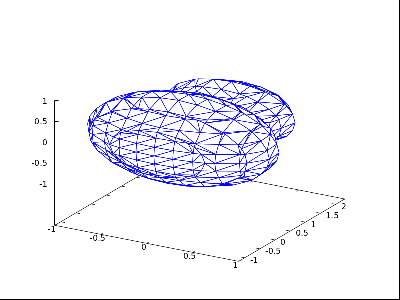 Categories: Package draw ·
- Graphic object: label
label ([string,x,y],...)
label ([string,x,y,z],...) ¶ -
Writes labels in 2D and 3D.
Colored labels work only with Gnuplot 4.3 and up.
This object is affected by the following graphic options:
label_alignment,label_orientationandcolor.2D
label([string,x,y])writes the string at point[x,y].Example:
(%i1) draw2d(yrange = [0.1,1.4], color = red, label(["Label in red",0,0.3]), color = "#0000ff", label(["Label in blue",0,0.6]), color = light_blue, label(["Label in light-blue",0,0.9], ["Another light-blue",0,1.2]) )$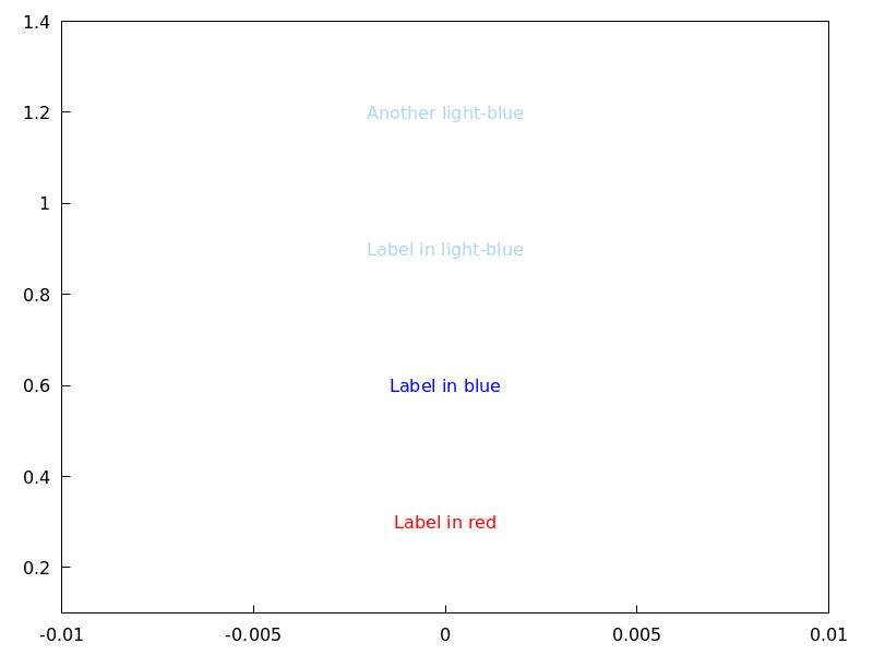
3D
label([string,x,y,z])writes the string at point[x,y,z].Example:
(%i1) draw3d(explicit(exp(sin(x)+cos(x^2)),x,-3,3,y,-3,3), color = red, label(["UP 1",-2,0,3], ["UP 2",1.5,0,4]), color = blue, label(["DOWN 1",2,0,-3]) )$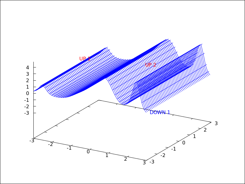 Categories: Package draw ·
- Graphic object: mesh (row_1,row_2,...) 
Draws a quadrangular mesh in 3D.
3D
Argument row_i is a list of n 3D points of the form
[[x_i1,y_i1,z_i1], ...,[x_in,y_in,z_in]], and all rows are of equal length. All these points define an arbitrary surface in 3D and in some sense it’s a generalization of theelevation_gridobject.This object is affected by the following graphic options:
line_type,line_width,color,key,wired_surface,enhanced3dandtransform.Examples:
A simple example.
(%i1) draw3d( mesh([[1,1,3], [7,3,1],[12,-2,4],[15,0,5]], [[2,7,8], [4,3,1],[10,5,8], [12,7,1]], [[-2,11,10],[6,9,5],[6,15,1], [20,15,2]])) $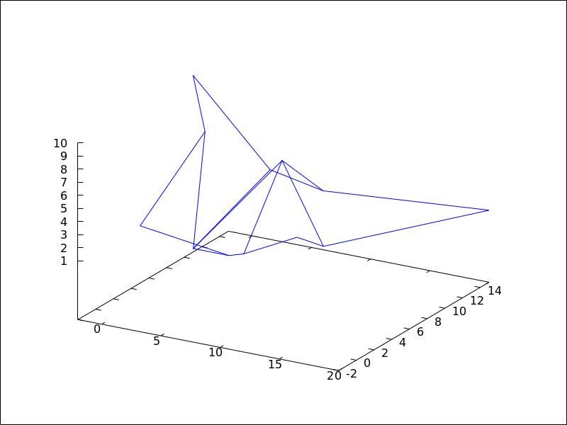
Plotting a triangle in 3D.
(%i1) draw3d( line_width = 2, mesh([[1,0,0],[0,1,0]], [[0,0,1],[0,0,1]])) $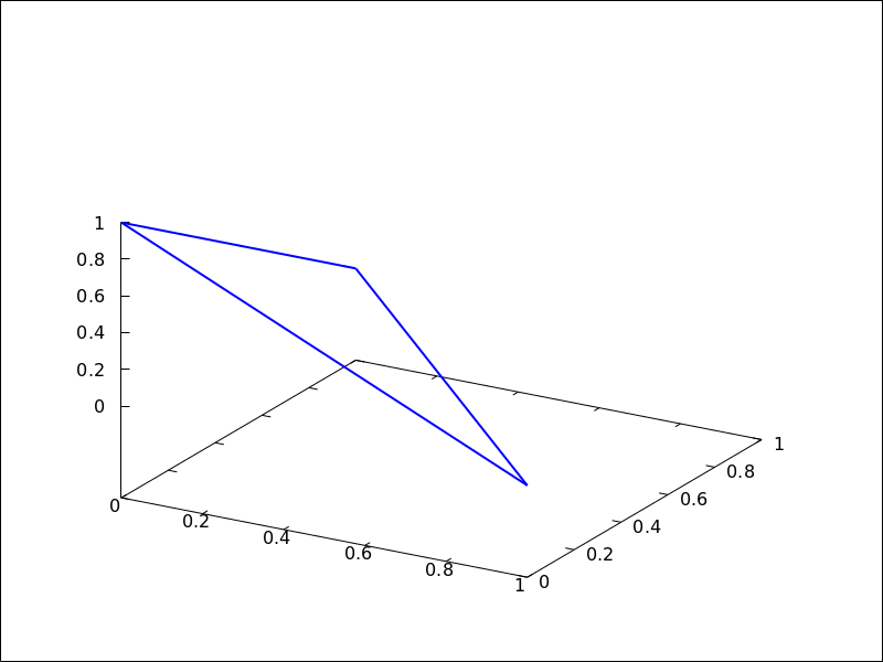
Two quadrilaterals.
(%i1) draw3d( surface_hide = true, line_width = 3, color = red, mesh([[0,0,0], [0,1,0]], [[2,0,2], [2,2,2]]), color = blue, mesh([[0,0,2], [0,1,2]], [[2,0,4], [2,2,4]])) $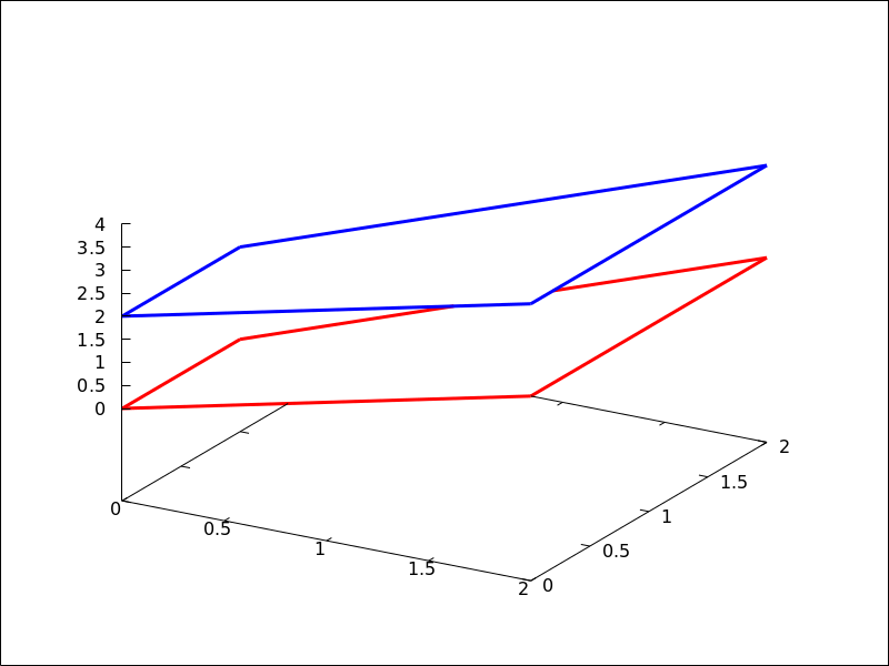 Categories: Package draw ·
- Graphic object: parametric
parametric (xfun,yfun,par,parmin,parmax)
parametric (xfun,yfun,zfun,par,parmin,parmax) ¶ -
Draws parametric functions in 2D and 3D.
This object is affected by the following graphic options:
nticks,line_width,line_type,key,colorandenhanced3d.2D
The command
parametric(xfun, yfun, par, parmin, parmax)plots the parametric function[xfun, yfun], with parameter par taking values from parmin to parmax.Example:
(%i1) draw2d(explicit(exp(x),x,-1,3), color = red, key = "This is the parametric one!!", parametric(2*cos(rrr),rrr^2,rrr,0,2*%pi))$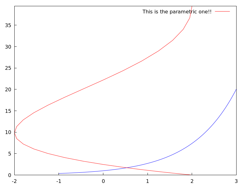
3D
parametric(xfun, yfun, zfun, par, parmin, parmax)plots the parametric curve[xfun, yfun, zfun], with parameter par taking values from parmin to parmax.Example:
(%i1) draw3d(explicit(exp(sin(x)+cos(x^2)),x,-3,3,y,-3,3), color = royalblue, parametric(cos(5*u)^2,sin(7*u),u-2,u,0,2), color = turquoise, line_width = 2, parametric(t^2,sin(t),2+t,t,0,2), surface_hide = true, title = "Surface & curves" )$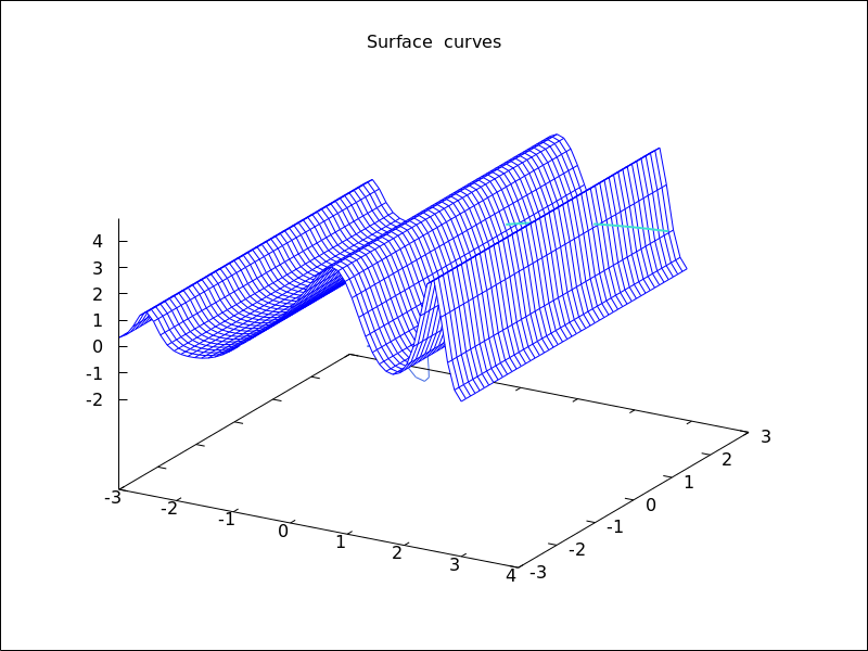 Categories: Package draw ·
- Graphic object: parametric_surface (xfun, yfun, zfun, par1, par1min, par1max, par2, par2min, par2max) 
Draws parametric surfaces in 3D.
3D
The command
parametric_surface(xfun, yfun, zfun, par1, par1min, par1max, par2, par2min, par2max)plots the parametric surface[xfun, yfun, zfun], with parameter par1 taking values from par1min to par1max and parameter par2 taking values from par2min to par2max.This object is affected by the following graphic options:
draw_realpart,xu_grid,yv_grid,line_type,line_width,key,wired_surface,enhanced3dandcolor.Example:
(%i1) draw3d(title = "Sea shell", xu_grid = 100, yv_grid = 25, view = [100,20], surface_hide = true, parametric_surface(0.5*u*cos(u)*(cos(v)+1), 0.5*u*sin(u)*(cos(v)+1), u*sin(v) - ((u+3)/8*%pi)^2 - 20, u, 0, 13*%pi, v, -%pi, %pi) )$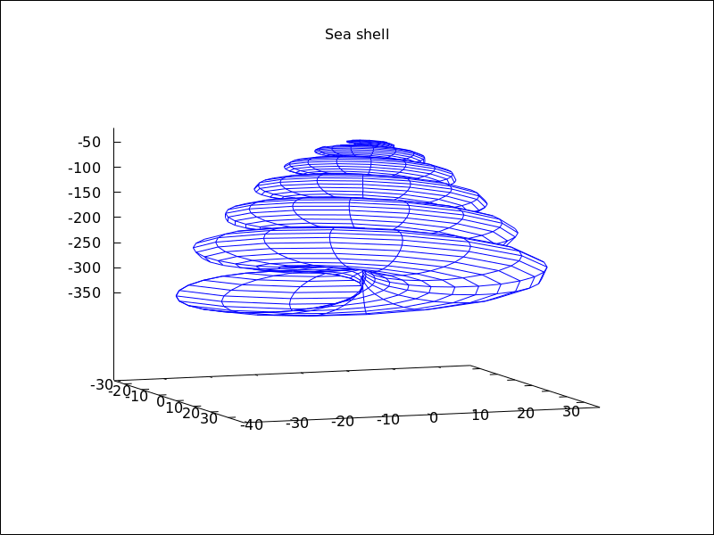 Categories: Package draw ·
- Graphic object: points
points ([[x1,y1], [x2,y2],...])
points ([x1,x2,...], [y1,y2,...])
points ([y1,y2,...])
points ([[x1,y1,z1], [x2,y2,z2],...])
points ([x1,x2,...], [y1,y2,...], [z1,z2,...])
points (matrix)
points (1d_y_array)
points (1d_x_array, 1d_y_array)
points (1d_x_array, 1d_y_array, 1d_z_array)
points (2d_xy_array)
points (2d_xyz_array) ¶ -
Draws points in 2D and 3D.
This object is affected by the following graphic options:
point_size,point_type,points_joined,line_width,key,line_typeandcolor. In 3D mode, it is also affected byenhanced3d2D
points ([[x1,y1], [x2,y2],...])orpoints ([x1,x2,...], [y1,y2,...])plots points[x1,y1],[x2,y2], etc. If abscissas are not given, they are set to consecutive positive integers, so thatpoints ([y1,y2,...])draws points[1,y1],[2,y2], etc. If matrix is a two-column or two-row matrix,points (matrix)draws the associated points. If matrix is an one-column or one-row matrix, abscissas are assigned automatically.If 1d_y_array is a 1D lisp array of numbers,
points (1d_y_array)plots them setting abscissas to consecutive positive integers.points (1d_x_array, 1d_y_array)plots points with their coordinates taken from the two arrays passed as arguments. If 2d_xy_array is a 2D array with two columns, or with two rows,points (2d_xy_array)plots the corresponding points on the plane.Examples:
Two types of arguments for
points, a list of pairs and two lists of separate coordinates.(%i1) draw2d( key = "Small points", points(makelist([random(20),random(50)],k,1,10)), point_type = circle, point_size = 3, points_joined = true, key = "Great points", points(makelist(k,k,1,20),makelist(random(30),k,1,20)), point_type = filled_down_triangle, key = "Automatic abscissas", color = red, points([2,12,8]))$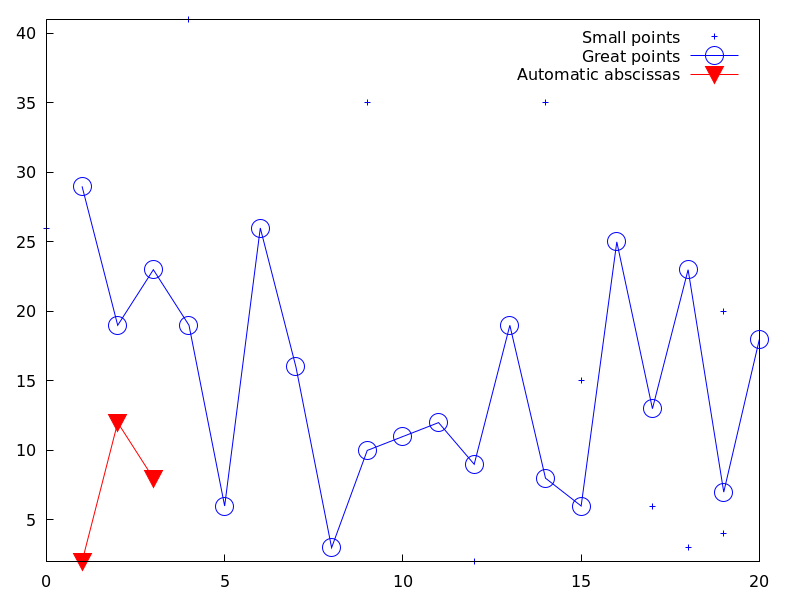
Drawing impulses.
(%i1) draw2d( points_joined = impulses, line_width = 2, color = red, points(makelist([random(20),random(50)],k,1,10)))$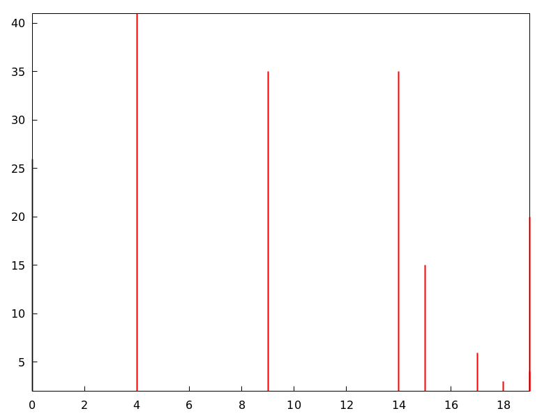
Array with ordinates.
(%i1) a: make_array (flonum, 100) $ (%i2) for i:0 thru 99 do a[i]: random(1.0) $ (%i3) draw2d(points(a)) $
Two arrays with separate coordinates.
(%i1) x: make_array (flonum, 100) $ (%i2) y: make_array (fixnum, 100) $ (%i3) for i:0 thru 99 do ( x[i]: float(i/100), y[i]: random(10) ) $ (%i4) draw2d(points(x, y)) $
A two-column 2D array.
(%i1) xy: make_array(flonum, 100, 2) $ (%i2) for i:0 thru 99 do ( xy[i, 0]: float(i/100), xy[i, 1]: random(10) ) $ (%i3) draw2d(points(xy)) $
Drawing an array filled with function
read_array.(%i1) a: make_array(flonum,100) $ (%i2) read_array (file_search ("pidigits.data"), a) $ (%i3) draw2d(points(a)) $3D
points([[x1, y1, z1], [x2, y2, z2], ...])orpoints([x1, x2, ...], [y1, y2, ...], [z1, z2,...])plots points[x1, y1, z1],[x2, y2, z2], etc. If matrix is a three-column or three-row matrix,points (matrix)draws the associated points.When arguments are lisp arrays,
points (1d_x_array, 1d_y_array, 1d_z_array)takes coordinates from the three 1D arrays. If 2d_xyz_array is a 2D array with three columns, or with three rows,points (2d_xyz_array)plots the corresponding points.Examples:
One tridimensional sample,
(%i1) load ("numericalio")$ (%i2) s2 : read_matrix (file_search ("wind.data"))$ (%i3) draw3d(title = "Daily average wind speeds", point_size = 2, points(args(submatrix (s2, 4, 5))) )$Two tridimensional samples,
(%i1) load ("numericalio")$ (%i2) s2 : read_matrix (file_search ("wind.data"))$ (%i3) draw3d( title = "Daily average wind speeds. Two data sets", point_size = 2, key = "Sample from stations 1, 2 and 3", points(args(submatrix (s2, 4, 5))), point_type = 4, key = "Sample from stations 1, 4 and 5", points(args(submatrix (s2, 2, 3))) )$Unidimensional arrays,
(%i1) x: make_array (fixnum, 10) $ (%i2) y: make_array (fixnum, 10) $ (%i3) z: make_array (fixnum, 10) $ (%i4) for i:0 thru 9 do ( x[i]: random(10), y[i]: random(10), z[i]: random(10) ) $ (%i5) draw3d(points(x,y,z)) $
Bidimensional colored array,
(%i1) xyz: make_array(fixnum, 10, 3) $ (%i2) for i:0 thru 9 do ( xyz[i, 0]: random(10), xyz[i, 1]: random(10), xyz[i, 2]: random(10) ) $ (%i3) draw3d( enhanced3d = true, points_joined = true, points(xyz)) $
Color numbers explicitly specified by the user.
(%i1) pts: makelist([t,t^2,cos(t)], t, 0, 15)$ (%i2) col_num: makelist(k, k, 1, length(pts))$ (%i3) draw3d( enhanced3d = ['part(col_num,k),k], point_size = 3, point_type = filled_circle, points(pts))$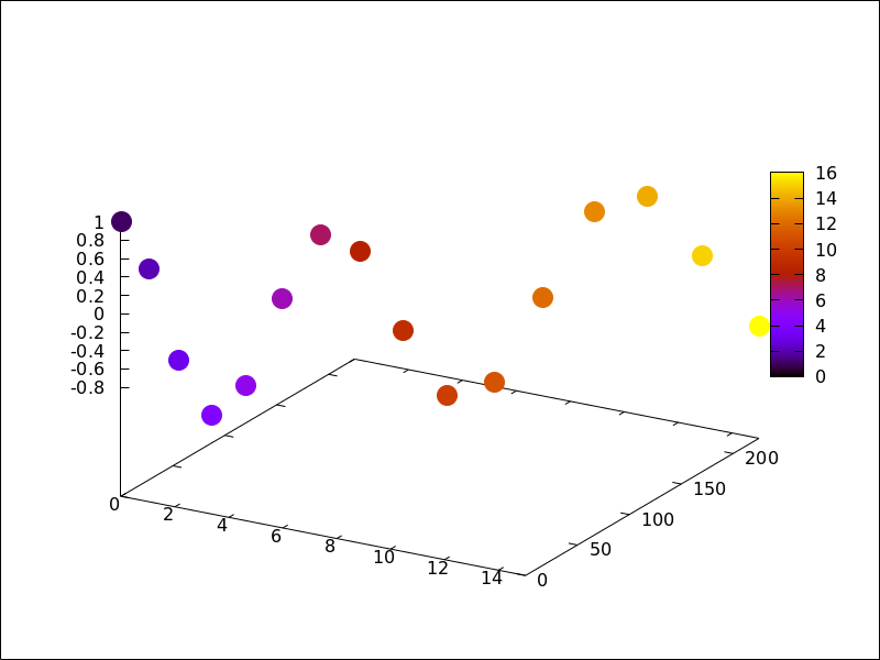 Categories: Package draw ·
- Graphic object: polar (radius,ang,minang,maxang) 
Draws 2D functions defined in polar coordinates.
2D
polar (radius,ang,minang,maxang)plots functionradius(ang)defined in polar coordinates, with variable ang taking values from minang to maxang.This object is affected by the following graphic options:
nticks,line_width,line_type,keyandcolor.Example:
(%i1) draw2d(user_preamble = "set grid polar", nticks = 200, xrange = [-5,5], yrange = [-5,5], color = blue, line_width = 3, title = "Hyperbolic Spiral", polar(10/theta,theta,1,10*%pi) )$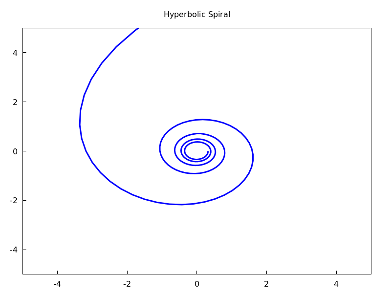 Categories: Package draw ·
- Graphic object: polygon
polygon ([[x1, y1], [x2, y2], …])
polygon ([x1, x2, …], [y1, y2, …]) ¶ -
Draws polygons in 2D.
2D
The commands
polygon([[x1, y1], [x2, y2], ...])orpolygon([x1, x2, ...], [y1, y2, ...])plot on the plane a polygon with vertices[x1, y1],[x2, y2], etc.This object is affected by the following graphic options:
transparent,fill_color,fill_density,border,line_width,key,line_typeandcolor.Example:
(%i1) draw2d(color = "#e245f0", line_width = 8, polygon([[3,2],[7,2],[5,5]]), border = false, fill_color = yellow, polygon([[5,2],[9,2],[7,5]]) )$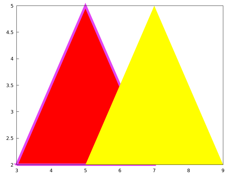 Categories: Package draw ·
- Graphic object: quadrilateral (point_1, point_2, point_3, point_4) 
Draws a quadrilateral.
2D
quadrilateral([x1, y1], [x2, y2], [x3, y3], [x4, y4])draws a quadrilateral with vertices[x1, y1],[x2, y2],[x3, y3], and[x4, y4].This object is affected by the following graphic options:
transparent,fill_color,border,line_width,key,xaxis_secondary,yaxis_secondary,line_type,transformandcolor.Example:
(%i1) draw2d( quadrilateral([1,1],[2,2],[3,-1],[2,-2]))$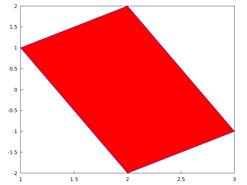
3D
quadrilateral([x1, y1, z1], [x2, y2, z2], [x3, y3, z3], [x4, y4, z4])draws a quadrilateral with vertices[x1, y1, z1],[x2, y2, z2],[x3, y3, z3], and[x4, y4, z4].This object is affected by the following graphic options:
line_type,line_width,color,key,enhanced3dandtransform.Categories: Package draw ·
- Graphic object: rectangle ([x1,y1], [x2,y2]) 
Draws rectangles in 2D.
2D
rectangle ([x1,y1], [x2,y2])draws a rectangle with opposite vertices[x1,y1]and[x2,y2].This object is affected by the following graphic options:
transparent,fill_color,border,line_width,key,line_typeandcolor.Example:
(%i1) draw2d(fill_color = red, line_width = 6, line_type = dots, transparent = false, fill_color = blue, rectangle([-2,-2],[8,-1]), /* opposite vertices */ transparent = true, line_type = solid, line_width = 1, rectangle([9,4],[2,-1.5]), xrange = [-3,10], yrange = [-3,4.5] )$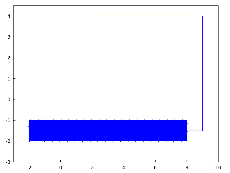 Categories: Package draw ·
- Graphic object: region (expr,var1,minval1,maxval1,var2,minval2,maxval2) 
Plots a region on the plane defined by inequalities.
2D expr is an expression formed by inequalities and boolean operators
and,or, andnot. The region is bounded by the rectangle defined by [minval1, maxval1] and [minval2, maxval2].This object is affected by the following graphic options:
fill_color,fill_density,key,x_voxelandy_voxel.Example:
(%i1) draw2d( x_voxel = 30, y_voxel = 30, region(x^2+y^2<1 and x^2+y^2 > 1/2, x, -1.5, 1.5, y, -1.5, 1.5));
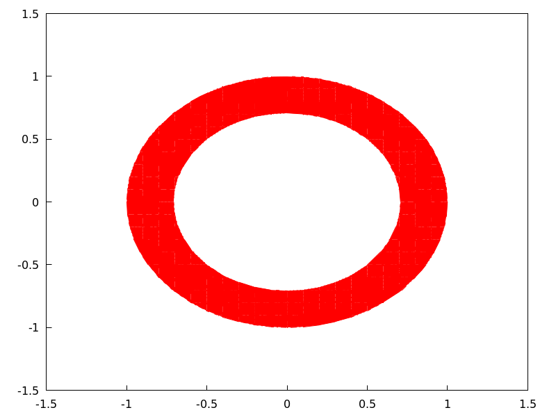
- Graphic object: spherical (radius, azi, minazi, maxazi, zen, minzen, maxzen) 
Draws 3D functions defined in spherical coordinates.
3D
spherical(radius, azi, minazi, maxazi, zen, minzen, maxzen)plots the functionradius(azi, zen)defined in spherical coordinates, with azimuth azi taking values from minazi to maxazi and zenith zen taking values from minzen to maxzen.This object is affected by the following graphic options:
xu_grid,yv_grid,line_type,key,wired_surface,enhanced3dandcolor.Example:
(%i1) draw3d(spherical(1,a,0,2*%pi,z,0,%pi))$
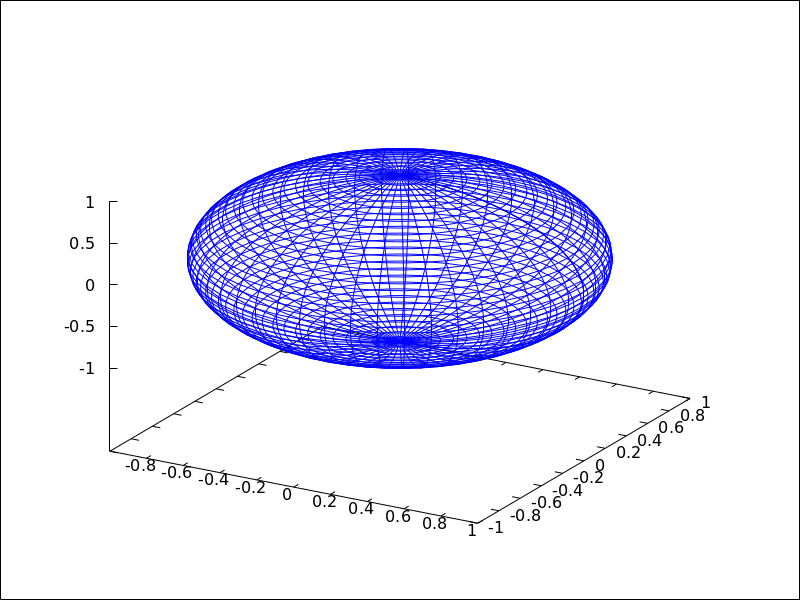 Categories: Package draw ·
- Graphic object: triangle (point_1, point_2, point_3) 
Draws a triangle.
2D
triangle ([x1,y1], [x2,y2], [x3,y3])draws a triangle with vertices[x1,y1],[x2,y2], and[x3,y3].This object is affected by the following graphic options:
transparent,fill_color,border,line_width,key,xaxis_secondary,yaxis_secondary,line_type,transformandcolor.Example:
(%i1) draw2d( triangle([1,1],[2,2],[3,-1]))$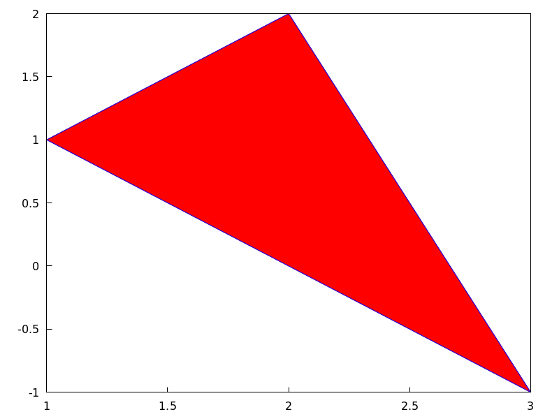
3D
triangle ([x1,y1,z1], [x2,y2,z2], [x3,y3,z3])draws a triangle with vertices[x1,y1,z1],[x2,y2,z2], and[x3,y3,z3].This object is affected by the following graphic options:
line_type,line_width,color,key,enhanced3dandtransform.Categories: Package draw ·
- Graphic object: tube (xfun,yfun,zfun,rfun,p,pmin,pmax) 
Draws a tube in 3D with varying diameter.
3D
[xfun,yfun,zfun]is the parametric curve with parameter p taking values from pmin to pmax. Circles of radius rfun are placed with their centers on the parametric curve and perpendicular to it.This object is affected by the following graphic options:
xu_grid,yv_grid,line_type,line_width,key,wired_surface,enhanced3d,colorandcapping.Example:
(%i1) draw3d( enhanced3d = true, xu_grid = 50, tube(cos(a), a, 0, cos(a/10)^2, a, 0, 4*%pi) )$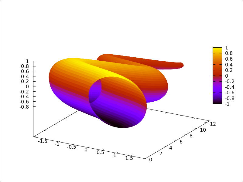 Categories: Package draw ·
- Graphic object: vector
vector ([x,y], [dx,dy])
vector ([x,y,z], [dx,dy,dz]) ¶ -
Draws vectors in 2D and 3D.
This object is affected by the following graphic options:
head_both,head_length,head_angle,head_type,line_width,line_type,keyandcolor.2D
vector([x,y], [dx,dy])plots vector[dx,dy]with origin in[x,y].Example:
(%i1) draw2d(xrange = [0,12], yrange = [0,10], head_length = 1, vector([0,1],[5,5]), /* default type */ head_type = 'empty, vector([3,1],[5,5]), head_both = true, head_type = 'nofilled, line_type = dots, vector([6,1],[5,5]))$
3D
vector([x,y,z], [dx,dy,dz])plots vector[dx,dy,dz]with origin in[x,y,z].Example:
(%i1) draw3d(color = cyan, vector([0,0,0],[1,1,1]/sqrt(3)), vector([0,0,0],[1,-1,0]/sqrt(2)), vector([0,0,0],[1,1,-2]/sqrt(6)) )$ Categories: Package draw ·
- Variable: draw_renderer 
Default value:
gnuplot_pipesThe only permitted values are
gnuplot_pipes,gnuplot,vtk,vtk6orvtk7. Whendraw_rendereris set tovtk, the VTK interface is used for draw.Categories: Package draw ·
Next: Functions and Variables for worldmap, Previous: Functions and Variables for draw, Up: Package draw [Contents][Index]
55.3 Functions and Variables for pictures
- Function: get_pixel (pic,x,y) 
Returns pixel from picture. Coordinates x and y range from 0 to
width-1andheight-1, respectively.Categories: Package draw ·
- Function: make_level_picture
make_level_picture (data)
make_level_picture (data,width,height) ¶ -
Returns a levels picture object.
make_level_picture (data)builds the picture object from matrix data.make_level_picture (data,width,height)builds the object from a list of numbers; in this case, both the width and the height must be given.The returned picture object contains the following four parts:
- symbol
level - image width
- image height
- an integer array with pixel data ranging from 0 to 255. Argument data must contain only numbers ranged from 0 to 255; negative numbers are substituted by 0, and those which are greater than 255 are set to 255.
Example:
Level picture from matrix.
(%i1) make_level_picture(matrix([3,2,5],[7,-9,3000])); (%o1) picture(level, 3, 2, {Array: #(3 2 5 7 0 255)})Level picture from numeric list.
(%i1) make_level_picture([-2,0,54,%pi],2,2); (%o1) picture(level, 2, 2, {Array: #(0 0 54 3)})Categories: Package draw · - symbol
- Function: make_rgb_picture (redlevel,greenlevel,bluelevel) 
Returns an rgb-coloured picture object. All three arguments must be levels picture; with red, green and blue levels.
The returned picture object contains the following four parts:
- symbol
rgb - image width
- image height
- an integer array of length 3*width*height with pixel data ranging from 0 to 255. Each pixel is represented by three consecutive numbers (red, green, blue).
Example:
(%i1) red: make_level_picture(matrix([3,2],[7,260])); (%o1) picture(level, 2, 2, {Array: #(3 2 7 255)}) (%i2) green: make_level_picture(matrix([54,23],[73,-9])); (%o2) picture(level, 2, 2, {Array: #(54 23 73 0)}) (%i3) blue: make_level_picture(matrix([123,82],[45,32.5698])); (%o3) picture(level, 2, 2, {Array: #(123 82 45 33)}) (%i4) make_rgb_picture(red,green,blue); (%o4) picture(rgb, 2, 2, {Array: #(3 54 123 2 23 82 7 73 45 255 0 33)})Categories: Package draw ·- symbol
- Function: negative_picture (pic) 
Returns the negative of a (level or rgb) picture.
Categories: Package draw ·
- Function: picture_equalp (x,y) 
Returns
truein case of equal pictures, andfalseotherwise.Categories: Package draw · Predicate functions ·
- Function: picturep (x) 
Returns
trueif the argument is a well formed image, andfalseotherwise.Categories: Package draw · Predicate functions ·
- Function: read_xpm (xpm_file) 
Reads a file in xpm and returns a picture object.
Categories: Package draw ·
- Function: rgb2level (pic) 
Transforms an rgb picture into a level one by averaging the red, green and blue channels.
Categories: Package draw ·
- Function: take_channel (im,color) 
If argument color is
red,greenorblue, functiontake_channelreturns the corresponding color channel of picture im. Example:(%i1) red: make_level_picture(matrix([3,2],[7,260])); (%o1) picture(level, 2, 2, {Array: #(3 2 7 255)}) (%i2) green: make_level_picture(matrix([54,23],[73,-9])); (%o2) picture(level, 2, 2, {Array: #(54 23 73 0)}) (%i3) blue: make_level_picture(matrix([123,82],[45,32.5698])); (%o3) picture(level, 2, 2, {Array: #(123 82 45 33)}) (%i4) make_rgb_picture(red,green,blue); (%o4) picture(rgb, 2, 2, {Array: #(3 54 123 2 23 82 7 73 45 255 0 33)}) (%i5) take_channel(%,'green); /* simple quote!!! */ (%o5) picture(level, 2, 2, {Array: #(54 23 73 0)})Categories: Package draw ·
Previous: Functions and Variables for pictures, Up: Package draw [Contents][Index]
55.4 Functions and Variables for worldmap
55.4.1 Variables and Functions
- Global variable: boundaries_array 
Default value:
falseboundaries_arrayis where the graphic objectgeomaplooks for boundaries coordinates.Each component of
boundaries_arrayis an array of floating point quantities, the coordinates of a polygonal segment or map boundary.See also
geomap.Categories: Package draw ·
- Function: numbered_boundaries (nlist) 
Draws a list of polygonal segments (boundaries), labeled by its numbers (
boundaries_arraycoordinates). This is of great help when building new geographical entities.Example:
Map of Europe labeling borders with their component number in
boundaries_array.(%i1) load("worldmap")$ (%i2) european_borders: region_boundaries(-31.81,74.92,49.84,32.06)$ (%i3) numbered_boundaries(european_borders)$Categories: Package draw ·
- Function: make_poly_continent
make_poly_continent (continent_name)
make_poly_continent (country_list) ¶ -
Makes the necessary polygons to draw a colored continent or a list of countries.
Example:
(%i1) load("worldmap")$ (%i2) /* A continent */ make_poly_continent(Africa)$ (%i3) apply(draw2d, %)$
(%i4) /* A list of countries */ make_poly_continent([Germany,Denmark,Poland])$ (%i5) apply(draw2d, %)$ Categories: Package draw ·
- Function: make_poly_country (country_name) 
Makes the necessary polygons to draw a colored country. If islands exist, one country can be defined with more than just one polygon.
Example:
(%i1) load("worldmap")$ (%i2) make_poly_country(India)$ (%i3) apply(draw2d, %)$ Categories: Package draw ·
- Function: make_polygon (nlist) 
Returns a
polygonobject from boundary indices. Argument nlist is a list of components ofboundaries_array.Example:
Bhutan is defined by boundary numbers 171, 173 and 1143, so that
make_polygon([171,173,1143])appends arrays of coordinatesboundaries_array[171],boundaries_array[173]andboundaries_array[1143]and returns apolygonobject suited to be plotted bydraw. To avoid an error message, arrays must be compatible in the sense that any two consecutive arrays have two coordinates in the extremes in common. In this example, the two first components ofboundaries_array[171]are equal to the last two coordinates ofboundaries_array[173], and the two first ofboundaries_array[173]are equal to the two first ofboundaries_array[1143]; in conclusion, boundary numbers 171, 173 and 1143 (in this order) are compatible and the colored polygon can be drawn.(%i1) load("worldmap")$ (%i2) Bhutan; (%o2) [[171, 173, 1143]] (%i3) boundaries_array[171]; (%o3) {Array: #(88.750549 27.14727 88.806351 27.25305 88.901367 27.282221 88.917877 27.321039)} (%i4) boundaries_array[173]; (%o4) {Array: #(91.659554 27.76511 91.6008 27.66666 91.598022 27.62499 91.631348 27.536381 91.765533 27.45694 91.775253 27.4161 92.007751 27.471939 92.11441 27.28583 92.015259 27.168051 92.015533 27.08083 92.083313 27.02277 92.112183 26.920271 92.069977 26.86194 91.997192 26.85194 91.915253 26.893881 91.916924 26.85416 91.8358 26.863331 91.712479 26.799999 91.542191 26.80444 91.492188 26.87472 91.418854 26.873329 91.371353 26.800831 91.307457 26.778049 90.682457 26.77417 90.392197 26.903601 90.344131 26.894159 90.143044 26.75333 89.98996 26.73583 89.841919 26.70138 89.618301 26.72694 89.636093 26.771111 89.360786 26.859989 89.22081 26.81472 89.110237 26.829161 88.921631 26.98777 88.873016 26.95499 88.867737 27.080549 88.843307 27.108601 88.750549 27.14727)} (%i5) boundaries_array[1143]; (%o5) {Array: #(91.659554 27.76511 91.666924 27.88888 91.65831 27.94805 91.338028 28.05249 91.314972 28.096661 91.108856 27.971109 91.015808 27.97777 90.896927 28.05055 90.382462 28.07972 90.396088 28.23555 90.366074 28.257771 89.996353 28.32333 89.83165 28.24888 89.58609 28.139999 89.35997 27.87166 89.225517 27.795 89.125793 27.56749 88.971077 27.47361 88.917877 27.321039)} (%i6) Bhutan_polygon: make_polygon([171,173,1143])$ (%i7) draw2d(Bhutan_polygon)$ Categories: Package draw ·
- Function: region_boundaries (x1,y1,x2,y2) 
Detects polygonal segments of global variable
boundaries_arrayfully contained in the rectangle with vertices (x1,y1) -upper left- and (x2,y2) -bottom right-.Example:
Returns segment numbers for plotting southern Italy.
(%i1) load("worldmap")$ (%i2) region_boundaries(10.4,41.5,20.7,35.4); (%o2) [1846, 1863, 1864, 1881, 1888, 1894] (%i3) draw2d(geomap(%))$ Categories: Package draw ·
- Function: region_boundaries_plus (x1,y1,x2,y2) 
Detects polygonal segments of global variable
boundaries_arraycontaining at least one vertex in the rectangle defined by vertices (x1,y1) -upper left- and (x2,y2) -bottom right-.Example:
(%i1) load("worldmap")$ (%i2) region_boundaries_plus(10.4,41.5,20.7,35.4); (%o2) [1060, 1062, 1076, 1835, 1839, 1844, 1846, 1858, 1861, 1863, 1864, 1871, 1881, 1888, 1894, 1897] (%i3) draw2d(geomap(%))$ Categories: Package draw ·
55.4.2 Graphic objects
- Graphic object: geomap
geomap (numlist)
geomap (numlist,3Dprojection) ¶ -
Draws cartographic maps in 2D and 3D.
2D
This function works together with global variable
boundaries_array.Argument numlist is a list containing numbers or lists of numbers. All these numbers must be integers greater or equal than zero, representing the components of global array
boundaries_array.Each component of
boundaries_arrayis an array of floating point quantities, the coordinates of a polygonal segment or map boundary.geomap (numlist)flattens its arguments and draws the associated boundaries inboundaries_array.This object is affected by the following graphic options:
line_width,line_typeandcolor.Examples:
A simple map defined by hand:
(%i1) load("worldmap")$ (%i2) /* Vertices of boundary #0: {(1,1),(2,5),(4,3)} */ ( bnd0: make_array(flonum,6), bnd0[0]:1.0, bnd0[1]:1.0, bnd0[2]:2.0, bnd0[3]:5.0, bnd0[4]:4.0, bnd0[5]:3.0 )$ (%i3) /* Vertices of boundary #1: {(4,3),(5,4),(6,4),(5,1)} */ ( bnd1: make_array(flonum,8), bnd1[0]:4.0, bnd1[1]:3.0, bnd1[2]:5.0, bnd1[3]:4.0, bnd1[4]:6.0, bnd1[5]:4.0, bnd1[6]:5.0, bnd1[7]:1.0)$ (%i4) /* Vertices of boundary #2: {(5,1), (3,0), (1,1)} */ ( bnd2: make_array(flonum,6), bnd2[0]:5.0, bnd2[1]:1.0, bnd2[2]:3.0, bnd2[3]:0.0, bnd2[4]:1.0, bnd2[5]:1.0 )$ (%i5) /* Vertices of boundary #3: {(1,1), (4,3)} */ ( bnd3: make_array(flonum,4), bnd3[0]:1.0, bnd3[1]:1.0, bnd3[2]:4.0, bnd3[3]:3.0)$ (%i6) /* Vertices of boundary #4: {(4,3), (5,1)} */ ( bnd4: make_array(flonum,4), bnd4[0]:4.0, bnd4[1]:3.0, bnd4[2]:5.0, bnd4[3]:1.0)$ (%i7) /* Pack all together in boundaries_array */ ( boundaries_array: make_array(any,5), boundaries_array[0]: bnd0, boundaries_array[1]: bnd1, boundaries_array[2]: bnd2, boundaries_array[3]: bnd3, boundaries_array[4]: bnd4 )$ (%i8) draw2d(geomap([0,1,2,3,4]))$
The auxiliary package
worldmapsets the global variableboundaries_arrayto real world boundaries in (longitude, latitude) coordinates. These data are in the public domain and come from https://web.archive.org/web/20100310124019/http://www-cger.nies.go.jp/grid-e/gridtxt/grid19.html. Packageworldmapdefines also boundaries for countries, continents and coastlines as lists with the necessary components ofboundaries_array(see fileshare/draw/worldmap.macfor more information). Packageworldmapautomatically loads packageworldmap.(%i1) load("worldmap")$ (%i2) c1: gr2d(geomap([Canada,United_States, Mexico,Cuba]))$ (%i3) c2: gr2d(geomap(Africa))$ (%i4) c3: gr2d(geomap([Oceania,China,Japan]))$ (%i5) c4: gr2d(geomap([France,Portugal,Spain, Morocco,Western_Sahara]))$ (%i6) draw(columns = 2, c1,c2,c3,c4)$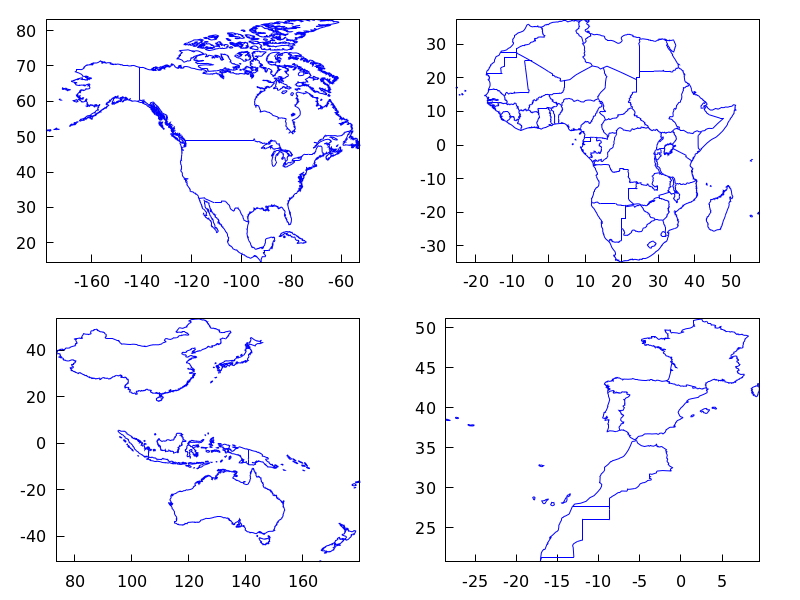
Package
worldmapis also useful for plotting countries as polygons. In this case, graphic objectgeomapis no longer necessary and thepolygonobject is used instead. Since lists are now used and not arrays, maps rendering will be slower. See alsomake_poly_countryandmake_poly_continentto understand the following code.(%i1) load("worldmap")$ (%i2) mymap: append( [color = white], /* borders are white */ [fill_color = red], make_poly_country(Bolivia), [fill_color = cyan], make_poly_country(Paraguay), [fill_color = green], make_poly_country(Colombia), [fill_color = blue], make_poly_country(Chile), [fill_color = "#23ab0f"], make_poly_country(Brazil), [fill_color = goldenrod], make_poly_country(Argentina), [fill_color = "midnight-blue"], make_poly_country(Uruguay))$ (%i3) apply(draw2d, mymap)$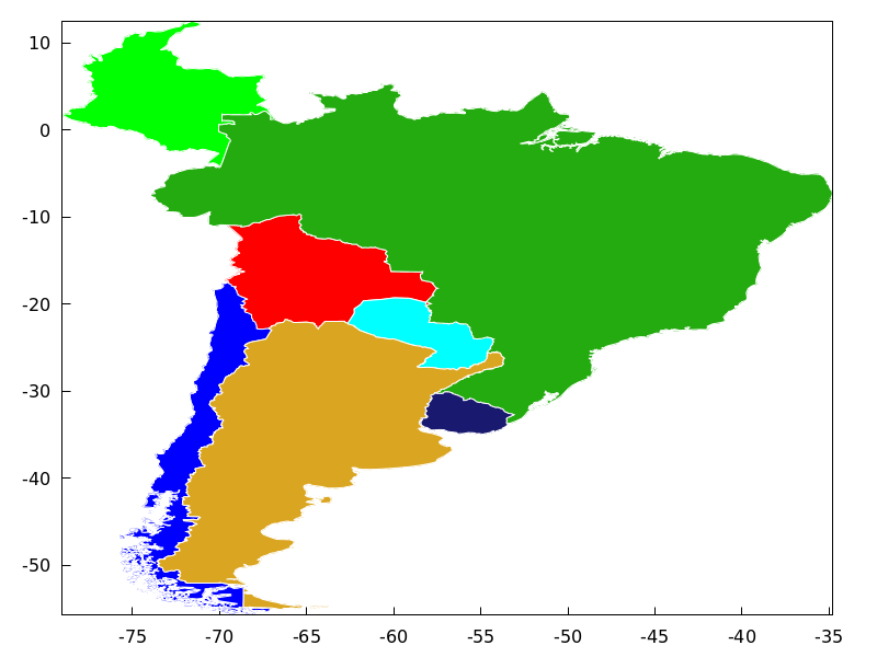
3D
geomap (numlist)projects map boundaries on the sphere of radius 1 centered at (0,0,0). It is possible to change the sphere or the projection type by usinggeomap (numlist,3Dprojection).Available 3D projections:
-
[spherical_projection,x,y,z,r]: projects map boundaries on the sphere of radius r centered at (x,y,z).(%i1) load("worldmap")$ (%i2) draw3d(geomap(Australia), /* default projection */ geomap(Australia, [spherical_projection,2,2,2,3]))$
-
[cylindrical_projection,x,y,z,r,rc]: re-projects spherical map boundaries on the cylinder of radius rc and axis passing through the poles of the globe of radius r centered at (x,y,z).(%i1) load("worldmap")$ (%i2) draw3d(geomap([America_coastlines,Eurasia_coastlines], [cylindrical_projection,2,2,2,3,4]))$
-
[conic_projection,x,y,z,r,alpha]: re-projects spherical map boundaries on the cones of angle alpha, with axis passing through the poles of the globe of radius r centered at (x,y,z). Both the northern and southern cones are tangent to sphere.(%i1) load("worldmap")$ (%i2) draw3d(geomap(World_coastlines, [conic_projection,0,0,0,1,90]))$
See also https://riotorto.users.sourceforge.net/Maxima/gnuplot/geomap/ for more elaborated examples.
Categories: Package draw · -
Next: Package dynamics, Previous: Package draw [Contents][Index]
56 Package drawdf
Next: Functions and Variables for drawdf, Previous: Package drawdf, Up: Package drawdf [Contents][Index]
56.1 Introduction to drawdf
The function drawdf draws the direction field of a first-order
Ordinary Differential Equation (ODE) or a system of two autonomous
first-order ODE’s.
Since this is an additional package, in order to use it you must first
load it with load("drawdf"). Drawdf is built upon the draw
package, which requires Gnuplot 4.2.
To plot the direction field of a single ODE, the ODE must be written in the form:
dy
-- = F(x,y)
dx
and the function F should be given as the argument for
drawdf. If the independent and dependent variables are not x,
and y, as in the equation above, then those two variables should
be named explicitly in a list given as an argument to the drawdf command
(see the examples).
To plot the direction field of a set of two autonomous ODE’s, they must be written in the form
dx dy
-- = G(x,y) -- = F(x,y)
dt dt
and the argument for drawdf should be a list with the two
functions G and F, in that order; namely, the first
expression in the list will be taken to be the time derivative of the
variable represented on the horizontal axis, and the second expression
will be the time derivative of the variable represented on the vertical
axis. Those two variables do not have to be x and y, but if
they are not, then the second argument given to drawdf must be another
list naming the two variables, first the one on the horizontal axis and
then the one on the vertical axis.
If only one ODE is given, drawdf will implicitly admit
x=t, and G(x,y)=1, transforming the non-autonomous
equation into a system of two autonomous equations.
Previous: Introduction to drawdf, Up: Package drawdf [Contents][Index]
56.2 Functions and Variables for drawdf
56.2.1 Functions
- Function: drawdf
drawdf (dydx, ...options and objects...)
drawdf (dvdu, [u,v], ...options and objects...)
drawdf (dvdu, [u,umin,umax], [v,vmin,vmax], ...options and objects...)
drawdf ([dxdt,dydt], ...options and objects...)
drawdf ([dudt,dvdt], [u,v], ...options and objects...)
drawdf ([dudt,dvdt], [u,umin,umax], [v,vmin,vmax], ...options and objects...) ¶ -
Function
drawdfdraws a 2D direction field with optional solution curves and other graphics using thedrawpackage.The first argument specifies the derivative(s), and must be either an expression or a list of two expressions. dydx, dxdt and dydt are expressions that depend on x and y. dvdu, dudt and dvdt are expressions that depend on u and v.
If the independent and dependent variables are not x and y, then their names must be specified immediately following the derivative(s), either as a list of two names
[u,v], or as two lists of the form[u,umin,umax]and[v,vmin,vmax].The remaining arguments are graphic options, graphic objects, or lists containing graphic options and objects, nested to arbitrary depth. The set of graphic options and objects supported by
drawdfis a superset of those supported bydraw2dandgr2dfrom thedrawpackage.The arguments are interpreted sequentially: graphic options affect all following graphic objects. Furthermore, graphic objects are drawn on the canvas in order specified, and may obscure graphics drawn earlier. Some graphic options affect the global appearance of the scene.
The additional graphic objects supported by
drawdfinclude:solns_at,points_at,saddles_at,soln_at,point_at, andsaddle_at.The additional graphic options supported by
drawdfinclude:field_degree,soln_arrows,field_arrows,field_grid,field_color,show_field,tstep,nsteps,duration,direction,field_tstep,field_nsteps, andfield_duration.Commonly used graphic objects inherited from the
drawpackage include:explicit,implicit,parametric,polygon,points,vector,label, and all others supported bydraw2dandgr2d.Commonly used graphic options inherited from the
drawpackage include:
points_joined,color,point_type,point_size,line_width,line_type,key,title,xlabel,ylabel,user_preamble,terminal,dimensions,file_name, and all others supported bydraw2dandgr2d.See also
draw2d,rk,desolveandode2.Users of wxMaxima or Imaxima may optionally use
wxdrawdf, which is identical todrawdfexcept that the graphics are drawn within the notebook usingwxdraw.To make use of this function, write first
load("drawdf").Examples:
(%i1) load("drawdf")$ (%i2) drawdf(exp(-x)+y)$ /* default vars: x,y */ (%i3) drawdf(exp(-t)+y, [t,y])$ /* default range: [-10,10] */ (%i4) drawdf([y,-9*sin(x)-y/5], [x,1,5], [y,-2,2])$For backward compatibility,
drawdfaccepts most of the parameters supported by plotdf.(%i5) drawdf(2*cos(t)-1+y, [t,y], [t,-5,10], [y,-4,9], [trajectory_at,0,0])$soln_atandsolns_atdraw solution curves passing through the specified points, using a slightly enhanced 4th-order Runge Kutta numerical integrator.(%i6) drawdf(2*cos(t)-1+y, [t,-5,10], [y,-4,9], solns_at([0,0.1],[0,-0.1]), color=blue, soln_at(0,0))$field_degree=2causes the field to be composed of quadratic splines, based on the first and second derivatives at each grid point.field_grid=[COLS,ROWS]specifies the number of columns and rows in the grid.(%i7) drawdf(2*cos(t)-1+y, [t,-5,10], [y,-4,9], field_degree=2, field_grid=[20,15], solns_at([0,0.1],[0,-0.1]), color=blue, soln_at(0,0))$soln_arrows=trueadds arrows to the solution curves, and (by default) removes them from the direction field. It also changes the default colors to emphasize the solution curves.(%i8) drawdf(2*cos(t)-1+y, [t,-5,10], [y,-4,9], soln_arrows=true, solns_at([0,0.1],[0,-0.1],[0,0]))$duration=40specifies the time duration of numerical integration (default 10). Integration will also stop automatically if the solution moves too far away from the plotted region, or if the derivative becomes complex or infinite. Here we also specifyfield_degree=2to plot quadratic splines. The equations below model a predator-prey system.(%i9) drawdf([x*(1-x-y), y*(3/4-y-x/2)], [x,0,1.1], [y,0,1], field_degree=2, duration=40, soln_arrows=true, point_at(1/2,1/2), solns_at([0.1,0.2], [0.2,0.1], [1,0.8], [0.8,1], [0.1,0.1], [0.6,0.05], [0.05,0.4], [1,0.01], [0.01,0.75]))$field_degree='solnscauses the field to be composed of many small solution curves computed by 4th-order Runge Kutta, with better results in this case.(%i10) drawdf([x*(1-x-y), y*(3/4-y-x/2)], [x,0,1.1], [y,0,1], field_degree='solns, duration=40, soln_arrows=true, point_at(1/2,1/2), solns_at([0.1,0.2], [0.2,0.1], [1,0.8], [0.8,1], [0.1,0.1], [0.6,0.05], [0.05,0.4], [1,0.01], [0.01,0.75]))$saddles_atattempts to automatically linearize the equation at each saddle, and to plot a numerical solution corresponding to each eigenvector, including the separatrices.tstep=0.05specifies the maximum time step for the numerical integrator (the default is 0.1). Note that smaller time steps will sometimes be used in order to keep the x and y steps small. The equations below model a damped pendulum.(%i11) drawdf([y,-9*sin(x)-y/5], tstep=0.05, soln_arrows=true, point_size=0.5, points_at([0,0], [2*%pi,0], [-2*%pi,0]), field_degree='solns, saddles_at([%pi,0], [-%pi,0]))$show_field=falsesuppresses the field entirely.(%i12) drawdf([y,-9*sin(x)-y/5], tstep=0.05, show_field=false, soln_arrows=true, point_size=0.5, points_at([0,0], [2*%pi,0], [-2*%pi,0]), saddles_at([3*%pi,0], [-3*%pi,0], [%pi,0], [-%pi,0]))$drawdfpasses all unrecognized parameters todraw2dorgr2d, allowing you to combine the full power of thedrawpackage withdrawdf.(%i13) drawdf(x^2+y^2, [x,-2,2], [y,-2,2], field_color=gray, key="soln 1", color=black, soln_at(0,0), key="soln 2", color=red, soln_at(0,1), key="isocline", color=green, line_width=2, nticks=100, parametric(cos(t),sin(t),t,0,2*%pi))$drawdfaccepts nested lists of graphic options and objects, allowing convenient use of makelist and other function calls to generate graphics.(%i14) colors : ['red,'blue,'purple,'orange,'green]$ (%i15) drawdf([x-x*y/2, (x*y - 3*y)/4], [x,2.5,3.5], [y,1.5,2.5], field_color = gray, makelist([ key = concat("soln",k), color = colors[k], soln_at(3, 2 + k/20) ], k,1,5))$Categories: Package drawdf ·
Next: Package engineering-format, Previous: Package drawdf [Contents][Index]
57 Package dynamics
Next: Graphical analysis of discrete dynamical systems, Previous: Package dynamics, Up: Package dynamics [Contents][Index]
57.1 The dynamics package
Package dynamics includes functions for 3D visualization,
animations, graphical analysis of differential and difference equations
and numerical solution of differential equations. The functions for
differential equations are described in the section on Numerical Methods and the functions to plot the Mandelbrot and Julia
sets are described in the section on Plotting.
All the functions in this package will be loaded automatically the first time they are used.
Next: Visualization with VTK, Previous: The dynamics package, Up: Package dynamics [Contents][Index]
57.2 Graphical analysis of discrete dynamical systems
- Function: chaosgame ([[x1, y1]…[xm, ym]], [x0, y0], b, n, options, …); 
-
Implements the so-called chaos game: the initial point (x0, y0) is plotted and then one of the m points [x1, y1]…xm, ym] will be selected at random. The next point plotted will be on the segment from the previous point plotted to the point chosen randomly, at a distance from the random point which will be b times that segment’s length. The procedure is repeated n times. The options are the same as for
plot2d.Example. A plot of Sierpinsky’s triangle:
(%i1) chaosgame([[0, 0], [1, 0], [0.5, sqrt(3)/2]], [0.1, 0.1], 1/2, 30000, [style, dots]);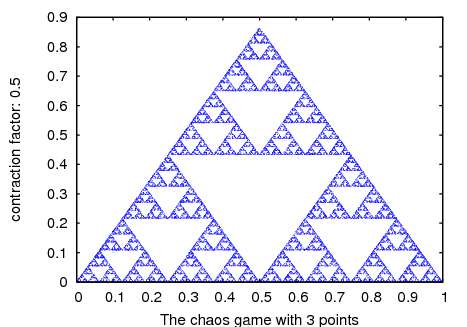 Categories: Package dynamics · Plotting ·
- Function: evolution (F, y0, n, …, options, …); 
-
Draws n+1 points in a two-dimensional graph, where the horizontal coordinates of the points are the integers 0, 1, 2, ..., n, and the vertical coordinates are the corresponding values y(n) of the sequence defined by the recurrence relation
y(n+1) = F(y(n))
With initial value y(0) equal to y0. F must be an expression that depends only on one variable (in the example, it depend on y, but any other variable can be used), y0 must be a real number and n must be a positive integer. This function accepts the same options as
plot2d.Example.
(%i1) evolution(cos(y), 2, 11);
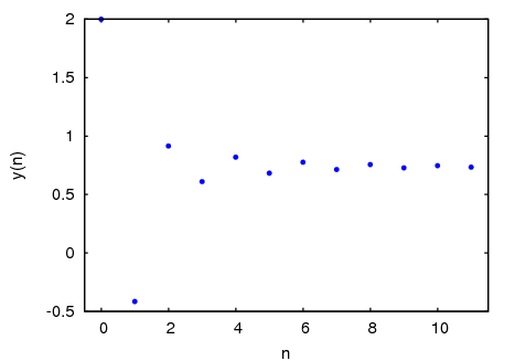 Categories: Package dynamics · Plotting ·
- Function: evolution2d ([F, G], [u, v], [u0, y0], n, options, …); 
-
Shows, in a two-dimensional plot, the first n+1 points in the sequence of points defined by the two-dimensional discrete dynamical system with recurrence relations
u(n+1) = F(u(n), v(n)) v(n+1) = G(u(n), v(n))
With initial values u0 and v0. F and G must be two expressions that depend only on two variables, u and v, which must be named explicitly in a list. The options are the same as for
plot2d.Example. Evolution of a two-dimensional discrete dynamical system:
(%i1) f: 0.6*x*(1+2*x)+0.8*y*(x-1)-y^2-0.9$ (%i2) g: 0.1*x*(1-6*x+4*y)+0.1*y*(1+9*y)-0.4$ (%i3) evolution2d([f,g], [x,y], [-0.5,0], 50000, [style,dots]);
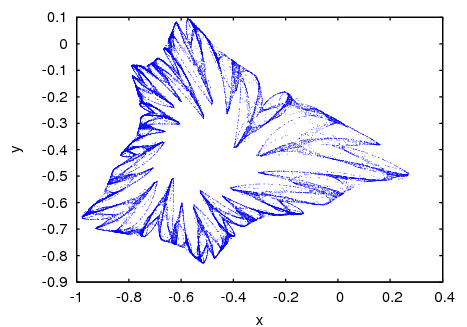
And an enlargement of a small region in that fractal:
(%i9) evolution2d([f,g], [x,y], [-0.5,0], 300000, [x,-0.8,-0.6], [y,-0.4,-0.2], [style, dots]);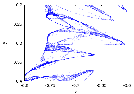 Categories: Package dynamics · Plotting ·
- Function: ifs ([r1, …, rm], [A1,…, Am], [[x1, y1], …, [xm, ym]], [x0, y0], n, options, …); 
-
Implements the Iterated Function System method. This method is similar to the method described in the function
chaosgame. but instead of shrinking the segment from the current point to the randomly chosen point, the 2 components of that segment will be multiplied by the 2 by 2 matrix Ai that corresponds to the point chosen randomly.The random choice of one of the m attractive points can be made with a non-uniform probability distribution defined by the weights r1,...,rm. Those weights are given in cumulative form; for instance if there are 3 points with probabilities 0.2, 0.5 and 0.3, the weights r1, r2 and r3 could be 2, 7 and 10. The options are the same as for
plot2d.Example. Barnsley’s fern, obtained with 4 matrices and 4 points:
(%i1) a1: matrix([0.85,0.04],[-0.04,0.85])$ (%i2) a2: matrix([0.2,-0.26],[0.23,0.22])$ (%i3) a3: matrix([-0.15,0.28],[0.26,0.24])$ (%i4) a4: matrix([0,0],[0,0.16])$ (%i5) p1: [0,1.6]$ (%i6) p2: [0,1.6]$ (%i7) p3: [0,0.44]$ (%i8) p4: [0,0]$ (%i9) w: [85,92,99,100]$ (%i10) ifs(w, [a1,a2,a3,a4], [p1,p2,p3,p4], [5,0], 50000, [style,dots]);
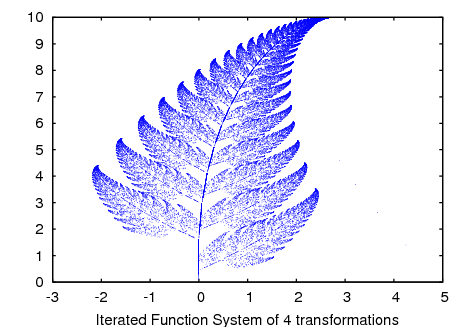 Categories: Package dynamics · Plotting ·
- Function: orbits (F, y0, n1, n2, [x, x0, xf, xstep], options, …); 
-
Draws the orbits diagram for a family of one-dimensional discrete dynamical systems, with one parameter x; that kind of diagram is used to study the bifurcations of an one-dimensional discrete system.
The function F(y) defines a sequence with a starting value of y0, as in the case of the function
evolution, but in this case that function will also depend on a parameter x that will take values in the interval from x0 to xf with increments of xstep. Each value used for the parameter x is shown on the horizontal axis. The vertical axis will show the n2 values of the sequence y(n1+1),..., y(n1+n2+1) obtained after letting the sequence evolve n1 iterations. In addition to the options accepted byplot2d, it accepts an option pixels that sets up the maximum number of different points that will be represented in the vertical direction.Example. Orbits diagram of the quadratic map, with a parameter a:
(%i1) orbits(x^2+a, 0, 50, 200, [a, -2, 0.25], [style, dots]);
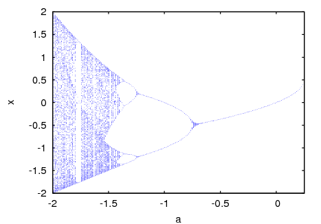
To enlarge the region around the lower bifurcation near x
=-1.25 use:(%i2) orbits(x^2+a, 0, 100, 400, [a,-1,-1.53], [x,-1.6,-0.8], [nticks, 400], [style,dots]);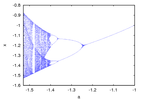 Categories: Package dynamics · Plotting ·
- Function: staircase (F, y0, n,options,…); 
-
Draws a staircase diagram for the sequence defined by the recurrence relation
y(n+1) = F(y(n))
The interpretation and allowed values of the input parameters is the same as for the function
evolution. A staircase diagram consists of a plot of the function F(y), together with the line G(y)=y. A vertical segment is drawn from the point (y0, y0) on that line until the point where it intersects the function F. From that point a horizontal segment is drawn until it reaches the point (y1, y1) on the line, and the procedure is repeated n times until the point (yn, yn) is reached. The options are the same as forplot2d.Example.
(%i1) staircase(cos(y), 1, 11, [y, 0, 1.2]);
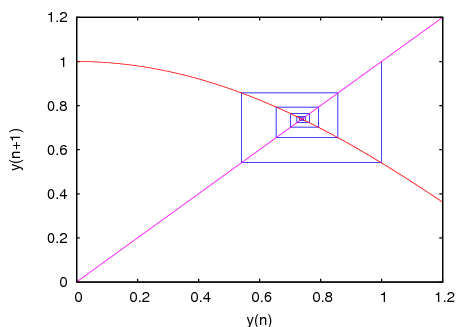 Categories: Package dynamics · Plotting ·
Previous: Graphical analysis of discrete dynamical systems, Up: Package dynamics [Contents][Index]
57.3 Visualization with VTK
Function scene creates 3D images and animations using the Visualization ToolKit (VTK) software. In order to use that function, Xmaxima and VTK should be installed in your system (including the TCL bindings of VTK, which in some system might come in a separate package).
- Function: scene (objects, …, options, …); 
-
Accepts an empty list or a list of several
objectsandoptions. The program launches Xmaxima, which opens an external window representing the given objects in a 3-dimensional space and applying the options given. Each object must belong to one of the following 4 classes: sphere, cube, cylinder or cone (seeScene objects). Objects are identified by giving their name or by a list in which the first element is the class name and the following elements are options for that object.Example. A hexagonal pyramid with a blue background:
(%i1) scene(cone, [background,"#9980e5"])$

By holding down the left button of the mouse while it is moved on the graphics window, the camera can be rotated showing different views of the pyramid. The two plot options
elevationandazimuthcan also be used to change the initial orientation of the viewing camera. The camera can be moved by holding the middle mouse button while moving it and holding the right-side mouse button while moving it up or down will zoom in or out.Each object option should be a list starting with the option name, followed by its value. The list of allowed options can be found in the
Scene object's optionssection.Example. This will show a sphere falling to the ground and bouncing off without losing any energy. To start or pause the animation, press the play/pause button.
(%i1) p: makelist ([0,0,2.1- 9.8*t^2/2], t, 0, 0.64, 0.01)$ (%i2) p: append (p, reverse(p))$ (%i3) ball: [sphere, [radius,0.1], [thetaresolution,20], [phiresolution,20], [position,0,0,2.1], [color,red], [animate,position,p]]$ (%i4) ground: [cube, [xlength,2], [ylength,2], [zlength,0.2], [position,0,0,-0.1],[color,violet]]$ (%i5) scene (ball, ground, restart)$
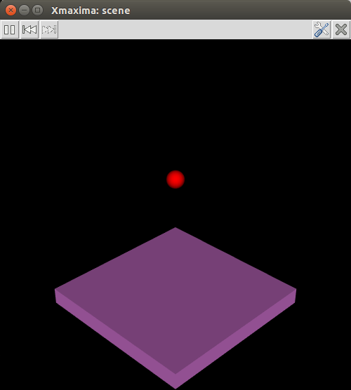
The restart option was used to make the animation restart automatically every time the last point in the position list is reached. The accepted values for the colors are the same as for the
coloroption of plot2d.Categories: Package dynamics · Plotting ·
57.3.1 Scene options
- Scene option: azimuth [azimuth, angle] 
Default value:
135The rotation of the camera on the horizontal (x, y) plane. angle must be a real number; an angle of 0 means that the camera points in the direction of the y axis and the x axis will appear on the right.
Categories: Package dynamics · Plotting ·
- Scene option: background [background, color] 
Default value:
blackThe color of the graphics window’s background. It accepts color names or hexadecimal red-green-blue strings (see the
coloroption of plot2d).Categories: Package dynamics · Plotting ·
- Scene option: elevation [elevation, angle] 
Default value:
30The vertical rotation of the camera. The angle must be a real number; an angle of 0 means that the camera points on the horizontal, and the default angle of 30 means that the camera is pointing 30 degrees down from the horizontal.
Categories: Package dynamics · Plotting ·
- Scene option: height [height, pixels] 
Default value:
500The height, in pixels, of the graphics window. pixels must be a positive integer number.
Categories: Package dynamics · Plotting ·
- Scene option: restart [restart, value] 
Default value:
falseA true value means that animations will restart automatically when the end of the list is reached. Writing just “restart” is equivalent to [restart, true].
Categories: Package dynamics · Plotting ·
- Scene option: tstep [tstep, time] 
Default value:
10The amount of time, in mili-seconds, between iterations among consecutive animation frames. time must be a real number.
Categories: Package dynamics · Plotting ·
- Scene option: width [width, pixels] 
Default value:
500The width, in pixels, of the graphics window. pixels must be a positive integer number.
Categories: Package dynamics · Plotting ·
- Scene option: windowname [windowtitle, name] 
Default value:
.scenename must be a string that can be used as the name of the Tk window created by Xmaxima for the
scenegraphics. The default value.sceneimplies that a new top level window will be created.Categories: Package dynamics · Plotting ·
- Scene option: windowtitle [windowtitle, name] 
Default value:
Xmaxima: scenename must be a string that will be written in the title of the window created by
scene.Categories: Package dynamics · Plotting ·
57.3.2 Scene objects
- Scene object: cone [cone, options] 
-
Creates a regular pyramid with height equal to 1 and a hexagonal base with vertices 0.5 units away from the axis. Options
heightandradiuscan be used to change those defaults and optionresolutioncan be used to change the number of edges of the base; higher values will make it look like a cone. By default, the axis will be along the x axis, the middle point of the axis will be at the origin and the vertex on the positive side of the x axis; use optionsorientationandcenterto change those defaults.Example. This shows a pyramid that starts rotating around the z axis when the play button is pressed.
(%i1) scene([cone, [orientation,0,30,0], [tstep,100], [animate,orientation,makelist([0,30,i],i,5,360,5)]], restart)$
Categories: Package dynamics · Plotting ·
- Scene object: cube [cube, options] 
-
A cube with edges of 1 unit and faces parallel to the xy, xz and yz planes. The lengths of the three edges can be changed with options
xlength,ylengthandzlength, turning it into a rectangular box and the faces can be rotated with optionorientation.Categories: Package dynamics · Plotting ·
- Scene object: cylinder [cylinder, options] 
-
Creates a regular prism with height equal to 1 and a hexagonal base with vertices 0.5 units away from the axis. Options
heightandradiuscan be used to change those defaults and optionresolutioncan be used to change the number of edges of the base; higher values will make it look like a cylinder. The default height can be changed with the optionheight. By default, the axis will be along the x axis and the middle point of the axis will be at the origin; use optionsorientationandcenterto change those defaults.Categories: Package dynamics · Plotting ·
- Scene object: sphere [sphere, options] 
-
A sphere with default radius of 0.5 units and center at the origin.
Categories: Package dynamics · Plotting ·
57.3.3 Scene object’s options
- Object option: animation [animation, property, positions] 
-
property should be one of the following 4 object’s properties:
origin,scale,positionororientationand positions should be a list of points. When the play button is pressed, the object property will be changed sequentially through all the values in the list, at intervals of time given by the optiontstep. The rewind button can be used to point at the start of the sequence making the animation restart after the play button is pressed again.See also
track.Categories: Package dynamics · Plotting ·
- Object option: capping [capping, number] 
Default value:
1In a cone or a cylinder, it defines whether the base (or bases) will be shown. A value of 1 for number makes the base visible and a value of 0 makes it invisible.
Categories: Package dynamics · Plotting ·
- Object option: center [center, point] 
Default value:
[0, 0, 0]The coordinates of the object’s geometric center, with respect to its
position. point can be a list with 3 real numbers, or 3 real numbers separated by commas. In a cylinder, cone or cube it will be at half its height and in a sphere at its center.Categories: Package dynamics · Plotting ·
- Object option: color [color, colorname] 
Default value:
whiteThe color of the object. It accepts color names or hexadecimal red-green-blue strings (see the
coloroption of plot2d).Categories: Package dynamics · Plotting ·
- Object option: endphi [endphi, angle] 
Default value:
180In a sphere phi is the angle on the vertical plane that passes through the z axis, measured from the positive part of the z axis. angle must be a number between 0 and 180 that sets the final value of phi at which the surface will end. A value smaller than 180 will eliminate a part of the sphere’s surface.
See also
startphiandphiresolution.Categories: Package dynamics · Plotting ·
- Object option: endtheta [endtheta, angle] 
Default value:
360In a sphere theta is the angle on the horizontal plane (longitude), measured from the positive part of the x axis. angle must be a number between 0 and 360 that sets the final value of theta at which the surface will end. A value smaller than 360 will eliminate a part of the sphere’s surface.
See also
startthetaandthetaresolution.Categories: Package dynamics · Plotting ·
- Object option: height [height, value] 
Default value:
1value must be a positive number which sets the height of a cone or a cylinder.
Categories: Package dynamics · Plotting ·
- Object option: linewidth [linewidth, value] 
Default value:
1The width of the lines, when option
wireframeis used. value must be a positive number.Categories: Package dynamics · Plotting ·
- Object option: opacity [opacity, value] 
Default value:
1value must be a number between 0 and 1. The lower the number, the more transparent the object will become. The default value of 1 means a completely opaque object.
Categories: Package dynamics · Plotting ·
- Object option: orientation [orientation, angles] 
Default value:
[0, 0, 0]Three angles by which the object will be rotated with respect to the three axis. angles can be a list with 3 real numbers, or 3 real numbers separated by commas. Example:
[0, 0, 90]rotates the x axis of the object to the y axis of the reference frame.Categories: Package dynamics · Plotting ·
- Object option: origin [origin, point] 
Default value:
[0, 0, 0]The coordinates of the object’s origin, with respect to which its other dimensions are defined. point can be a list with 3 real numbers, or 3 real numbers separated by commas.
Categories: Package dynamics · Plotting ·
- Object option: phiresolution [phiresolution, num] 
Default value:
The number of sub-intervals into which the phi angle interval from
startphitoendphiwill be divided. num must be a positive integer.Categories: Package dynamics · Plotting ·
- Object option: points [points] 
-
Only the vertices of the triangulation used to render the surface will be shown. Example:
[sphere, [points]]See also
surfaceandwireframe.Categories: Package dynamics · Plotting ·
- Object option: pointsize [pointsize, value] 
Default value:
1The size of the points, when option
pointsis used. value must be a positive number.Categories: Package dynamics · Plotting ·
- Object option: position [position, point] 
Default value:
[0, 0, 0]The coordinates of the object’s position. point can be a list with 3 real numbers, or 3 real numbers separated by commas.
Categories: Package dynamics · Plotting ·
- Object option: radius [radius, value] 
Default value:
0.5The radius or a sphere or the distance from the axis to the base’s vertices in a cylinder or a cone. value must be a positive number.
Categories: Package dynamics · Plotting ·
- Object option: resolution [resolution, number] 
Default value:
6number must be an integer greater than 2 that sets the number of edges in the base of a cone or a cylinder.
Categories: Package dynamics · Plotting ·
- Object option: scale [scale, factors] 
Default value:
[1, 1, 1]Three numbers by which the object will be scaled with respect to the three axis. factors can be a list with 3 real numbers, or 3 real numbers separated by commas. Example:
[2, 0.5, 1]enlarges the object to twice its size in the x direction, reduces the dimensions in the y direction to half and leaves the z dimensions unchanged.Categories: Package dynamics · Plotting ·
- Object option: startphi [startphi, angle] 
Default value:
0In a sphere phi is the angle on the vertical plane that passes through the z axis, measured from the positive part of the z axis. angle must be a number between 0 and 180 that sets the initial value of phi at which the surface will start. A value bigger than 0 will eliminate a part of the sphere’s surface.
See also
endphiandphiresolution.Categories: Package dynamics · Plotting ·
- Object option: starttheta [starttheta, angle] 
Default value:
0In a sphere theta is the angle on the horizontal plane (longitude), measured from the positive part of the x axis. angle must be a number between 0 and 360 that sets the initial value of theta at which the surface will start. A value bigger than 0 will eliminate a part of the sphere’s surface.
See also
endthetaandthetaresolution.Categories: Package dynamics · Plotting ·
- Object option: surface [surface] 
-
The surfaces of the object will be rendered and the lines and points of the triangulation used to build the surface will not be shown. This is the default behavior, which can be changed using either the option
pointsorwireframe.Categories: Package dynamics · Plotting ·
- Object option: thetaresolution [thetaresolution, num] 
Default value:
The number of sub-intervals into which the theta angle interval from
startthetatoendthetawill be divided. num must be a positive integer.See also
startthetaandendtheta.Categories: Package dynamics · Plotting ·
- Object option: track [track, positions] 
-
positions should be a list of points. When the play button is pressed, the object position will be changed sequentially through all the points in the list, at intervals of time given by the option
tstep, leaving behind a track of the object’s trajectory. The rewind button can be used to point at the start of the sequence making the animation restart after the play button is pressed again.Example. This will show the trajectory of a ball thrown with speed of 5 m/s, at an angle of 45 degrees, when the air resistance can be neglected:
(%i1) p: makelist ([0,4*t,4*t- 9.8*t^2/2], t, 0, 0.82, 0.01)$ (%i2) ball: [sphere, [radius,0.1], [color,red], [track,p]]$ (%i3) ground: [cube, [xlength,2], [ylength,4], [zlength,0.2], [position,0,1.5,-0.2],[color,green]]$ (%i4) scene (ball, ground)$See also
animation.Categories: Package dynamics · Plotting ·
- Object option: xlength [xlength, length] 
Default value:
1The height of a cube in the x direction. length must be a positive number. See also
ylengthandzlength.Categories: Package dynamics · Plotting ·
- Object option: ylength [ylength, length] 
Default value:
1The height of a cube in the y direction. length must be a positive number. See also
xlengthandzlength.Categories: Package dynamics · Plotting ·
- Object option: zlength [zlength, length] 
Default value:
1The height of a cube in z the direction. length must be a positive number. See also
xlengthandylength.Categories: Package dynamics · Plotting ·
- Object option: wireframe [wireframe] 
-
Only the edges of the triangulation used to render the surface will be shown. Example:
[cube, [wireframe]]Categories: Package dynamics · Plotting ·
Next: Package ezunits, Previous: Package dynamics [Contents][Index]
58 Package engineering-format
Engineering-format changes the way maxima outputs floating-point numbers
to the notation engineers are used to: a*10^b with b dividable by
three.
Previous: Package engineering-format, Up: Package engineering-format [Contents][Index]
58.1 Functions and Variables for engineering-format
- Option variable: engineering_format_floats 
Default value:
trueThis variable allows to temporarily switch off engineering-format.
(%i1) load("engineering-format"); (%o1) /home/gunter/src/maxima-code/share/contrib/engineering-for\ mat.lisp(%i2) float(sin(10)/10000); (%o2) - 54.40211108893698e-6
(%i3) engineering_format_floats:false$
(%i4) float(sin(10)/10000); (%o4) - 5.440211108893698e-5
See also
fpprintprecandfloat.
- Option variable: engineering_format_min 
Default value:
0.0The minimum absolute value that isn’t automatically converted to the engineering format. See also
engineering_format_maxandengineering_format_floats.(%i1) lst: float([.05,.5,5,500,5000,500000]); (%o1) [0.05, 0.5, 5.0, 500.0, 5000.0, 500000.0]
(%i2) load("engineering-format"); (%o2) /home/gunter/src/maxima-code/share/contrib/engineering-for\ mat.lisp(%i3) lst; (%o3) [50.0e-3, 500.0e-3, 5.0e+0, 500.0e+0, 5.0e+3, 500.0e+3]
(%i4) engineering_format_min:.1$ (%i5) engineering_format_max:1000$
(%i6) lst; (%o6) [50.0e-3, 0.5, 5.0, 500.0, 5.0e+3, 500.0e+3]
- Option variable: engineering_format_max 
Default value:
0.0The maximum absolute value that isn’t automatically converted to the engineering format. See also
engineering_format_minandengineering_format_floats.
Next: Package f90, Previous: Package engineering-format [Contents][Index]
59 Package ezunits
Next: Introduction to physical_constants, Previous: Package ezunits, Up: Package ezunits [Contents][Index]
59.1 Introduction to ezunits
ezunits is a package for working with dimensional quantities,
including some functions for dimensional analysis.
ezunits can carry out arithmetic operations on dimensional quantities and unit conversions.
The built-in units include Systeme Internationale (SI) and US customary units,
and other units can be declared.
See also physical_constants, a collection of physical constants.
load("ezunits") loads this package.
demo("ezunits") displays several examples.
The convenience function known_units returns a list of
the built-in and user-declared units,
while display_known_unit_conversions displays
the set of known conversions in an easy-to-read format.
An expression a ` b represents a dimensional quantity,
with a indicating a nondimensional quantity and b indicating the dimensional units.
A symbol can be used as a unit without declaring it as such;
unit symbols need not have any special properties.
The quantity and unit of an expression a ` b can
be extracted by the qty and units functions, respectively.
A symbol may be declared to be a dimensional quantity, with specified quantity or specified units or both.
An expression a ` b `` c converts from unit b to unit c.
ezunits has built-in conversions for SI base units,
SI derived units, and some non-SI units.
Unit conversions not already known to ezunits can be declared.
The unit conversions known to ezunits are specified by the
global variable known_unit_conversions,
which comprises built-in and user-defined conversions.
Conversions for products, quotients, and powers of units are
derived from the set of known unit conversions.
As Maxima generally prefers exact numbers (integers or rationals)
to inexact (float or bigfloat),
so ezunits preserves exact numbers when they appear
in dimensional quantities.
All built-in unit conversions are expressed in terms of exact numbers;
inexact numbers in declared conversions are coerced to exact.
There is no preferred system for display of units;
input units are not converted to other units
unless conversion is explicitly indicated.
ezunits recognizes the prefixes m-, k-, M, and G-
(for milli-, kilo-, mega-, and giga-)
as applied to SI base units and SI derived units,
but such prefixes are applied only when indicated by an explicit conversion.
Arithmetic operations on dimensional quantities are carried out by conventional rules for such operations.
- (x ` a) * (y ` b) is equal to (x * y) ` (a * b).
- (x ` a) + (y ` a) is equal to (x + y) ` a.
- (x ` a)^y is equal to x^y ` a^y when
yis nondimensional.
ezunits does not require that units in a sum have the same dimensions;
such terms are not added together, and no error is reported.
ezunits includes functions for elementary dimensional analysis,
namely the fundamental dimensions and fundamental units
of a dimensional quantity,
and computation of dimensionless quantities and natural units.
The functions for dimensional analysis were adapted from similar
functions in another package, written by Barton Willis.
For the purpose of dimensional analysis, a list of fundamental dimensions and an associated list of fundamental units are maintained; by default the fundamental dimensions are length, mass, time, charge, temperature, and quantity, and the fundamental units are the associated SI units, but other fundamental dimensions and units can be declared.
Next: Functions and Variables for ezunits, Previous: Introduction to ezunits, Up: Package ezunits [Contents][Index]
59.2 Introduction to physical_constants
physical_constants is a collection of physical constants,
copied from CODATA 2006 recommended values
(https://physics.nist.gov/cuu/Constants/).
load ("physical_constants") loads this package,
and loads ezunits also, if it is not already loaded.
A physical constant is represented as a symbol which has a property
which is the constant value.
The constant value is a dimensional quantity, as represented by ezunits.
The function constvalue fetches the constant value;
the constant value is not the ordinary value of the symbol,
so symbols of physical constants persist in evaluated expressions until their
values are fetched by constvalue.
physical_constants includes some auxiliary information,
namely, a description string for each constant,
an estimate of the error of its numerical value,
and a property for TeX display.
To identify physical constants, each symbol has the
physical_constant property;
propvars(physical_constant) therefore shows the list
of all such symbols.
physical_constants comprises the following constants.
%cspeed of light in vacuum
%mu_0magnetic constant
%e_0electric constant
%Z_0characteristic impedance of vacuum
%GNewtonian constant of gravitation
%hPlanck constant
%h_barPlanck constant
%m_PPlanck mass
%T_PPlanck temperature
%l_PPlanck length
%t_PPlanck time
%%eelementary charge
%Phi_0magnetic flux quantum
%G_0conductance quantum
%K_JJosephson constant
%R_Kvon Klitzing constant
%mu_BBohr magneton
%mu_Nnuclear magneton
%alphafine-structure constant
%R_infRydberg constant
%a_0Bohr radius
%E_hHartree energy
%ratio_h_mequantum of circulation
%m_eelectron mass
%N_AAvogadro constant
%m_uatomic mass constant
%FFaraday constant
%Rmolar gas constant
%%kBoltzmann constant
%V_mmolar volume of ideal gas
%n_0Loschmidt constant
%ratio_S0_RSackur-Tetrode constant (absolute entropy constant)
%sigmaStefan-Boltzmann constant
%c_1first radiation constant
%c_1Lfirst radiation constant for spectral radiance
%c_2second radiation constant
%bWien displacement law constant
%b_primeWien displacement law constant
Reference: https://physics.nist.gov/cuu/Constants/
Examples:
The list of all symbols which have the physical_constant property.
(%i1) load ("physical_constants")$
(%i2) propvars (physical_constant);
(%o2) [%c, %mu_0, %e_0, %Z_0, %G, %h, %h_bar, %m_P, %T_P, %l_P,
%t_P, %%e, %Phi_0, %G_0, %K_J, %R_K, %mu_B, %mu_N, %alpha,
%R_inf, %a_0, %E_h, %ratio_h_me, %m_e, %N_A, %m_u, %F, %R, %%k,
%V_m, %n_0, %ratio_S0_R, %sigma, %c_1, %c_1L, %c_2, %b, %b_prime]
Properties of the physical constant %c.
(%i1) load ("physical_constants")$
(%i2) constantp (%c);
(%o2) true
(%i3) get (%c, description);
(%o3) speed of light in vacuum
(%i4) constvalue (%c);
m
(%o4) 299792458 ` -
s
(%i5) get (%c, RSU);
(%o5) 0
(%i6) tex (%c);
$$c$$
(%o6) false
The energy equivalent of 1 pound-mass.
The symbol %c persists until its value is fetched by constvalue.
(%i1) load ("physical_constants")$
(%i2) m * %c^2;
2
(%o2) %c m
(%i3) %, m = 1 ` lbm;
2
(%o3) %c ` lbm
(%i4) constvalue (%);
2
lbm m
(%o4) 89875517873681764 ` ------
2
s
(%i5) E : % `` J;
Computing conversions to base units; may take a moment.
366838848464007200
(%o5) ------------------ ` J
9
(%i6) E `` GJ;
458548560580009
(%o6) --------------- ` GJ
11250000
(%i7) float (%);
(%o7) 4.0759872051556356e+7 ` GJ
Previous: Introduction to physical_constants, Up: Package ezunits [Contents][Index]
59.3 Functions and Variables for ezunits
- Operator: ` 
-
The dimensional quantity operator. An expression a ` b represents a dimensional quantity, with
aindicating a nondimensional quantity andbindicating the dimensional units. A symbol can be used as a unit without declaring it as such; unit symbols need not have any special properties. The quantity and unit of an expression a ` b can be extracted by theqtyandunitsfunctions, respectively.Arithmetic operations on dimensional quantities are carried out by conventional rules for such operations.
- (x ` a) * (y ` b) is equal to (x * y) ` (a * b).
- (x ` a) + (y ` a) is equal to (x + y) ` a.
- (x ` a)^y is equal to x^y ` a^y when
yis nondimensional.
ezunitsdoes not require that units in a sum have the same dimensions; such terms are not added together, and no error is reported.load ("ezunits")enables this operator.Examples:
SI (Systeme Internationale) units.
(%i1) load ("ezunits")$ (%i2) foo : 10 ` m; (%o2) 10 ` m (%i3) qty (foo); (%o3) 10 (%i4) units (foo); (%o4) m (%i5) dimensions (foo); (%o5) length"Customary" units.
(%i1) load ("ezunits")$ (%i2) bar : x ` acre; (%o2) x ` acre (%i3) dimensions (bar); 2 (%o3) length (%i4) fundamental_units (bar); 2 (%o4) mUnits ad hoc.
(%i1) load ("ezunits")$ (%i2) baz : 3 ` sheep + 8 ` goat + 1 ` horse; (%o2) 8 ` goat + 3 ` sheep + 1 ` horse (%i3) subst ([sheep = 3*goat, horse = 10*goat], baz); (%o3) 27 ` goat (%i4) baz2 : 1000`gallon/fortnight; gallon (%o4) 1000 ` --------- fortnight (%i5) subst (fortnight = 14*day, baz2); 500 gallon (%o5) --- ` ------ 7 dayArithmetic operations on dimensional quantities.
(%i1) load ("ezunits")$ (%i2) 100 ` kg + 200 ` kg; (%o2) 300 ` kg (%i3) 100 ` m^3 - 100 ` m^3; 3 (%o3) 0 ` m (%i4) (10 ` kg) * (17 ` m/s^2); kg m (%o4) 170 ` ---- 2 s (%i5) (x ` m) / (y ` s); x m (%o5) - ` - y s (%i6) (a ` m)^2; 2 2 (%o6) a ` mCategories: Package ezunits ·
- Operator: `` 
-
The unit conversion operator. An expression a ` b `` c converts from unit
bto unitc.ezunitshas built-in conversions for SI base units, SI derived units, and some non-SI units. Unit conversions not already known toezunitscan be declared. The unit conversions known toezunitsare specified by the global variableknown_unit_conversions, which comprises built-in and user-defined conversions. Conversions for products, quotients, and powers of units are derived from the set of known unit conversions.There is no preferred system for display of units; input units are not converted to other units unless conversion is explicitly indicated.
ezunitsdoes not attempt to simplify units by prefixes (milli-, centi-, deci-, etc) unless such conversion is explicitly indicated.load ("ezunits")enables this operator.Examples:
The set of known unit conversions.
(%i1) load ("ezunits")$ (%i2) display2d : false$ (%i3) known_unit_conversions; (%o3) {acre = 4840*yard^2,Btu = 1055*J,cfm = feet^3/minute, cm = m/100,day = 86400*s,feet = 381*m/1250,ft = feet, g = kg/1000,gallon = 757*l/200,GHz = 1000000000*Hz, GOhm = 1000000000*Ohm,GPa = 1000000000*Pa, GWb = 1000000000*Wb,Gg = 1000000*kg,Gm = 1000000000*m, Gmol = 1000000*mol,Gs = 1000000000*s,ha = hectare, hectare = 100*m^2,hour = 3600*s,Hz = 1/s,inch = feet/12, km = 1000*m,kmol = 1000*mol,ks = 1000*s,l = liter, lbf = pound_force,lbm = pound_mass,liter = m^3/1000, metric_ton = Mg,mg = kg/1000000,MHz = 1000000*Hz, microgram = kg/1000000000,micrometer = m/1000000, micron = micrometer,microsecond = s/1000000, mile = 5280*feet,minute = 60*s,mm = m/1000, mmol = mol/1000,month = 2629800*s,MOhm = 1000000*Ohm, MPa = 1000000*Pa,ms = s/1000,MWb = 1000000*Wb, Mg = 1000*kg,Mm = 1000000*m,Mmol = 1000000000*mol, Ms = 1000000*s,ns = s/1000000000,ounce = pound_mass/16, oz = ounce,Ohm = s*J/C^2, pound_force = 32*ft*pound_mass/s^2, pound_mass = 200*kg/441,psi = pound_force/inch^2, Pa = N/m^2,week = 604800*s,Wb = J/A,yard = 3*feet, year = 31557600*s,C = s*A,F = C^2/J,GA = 1000000000*A, GC = 1000000000*C,GF = 1000000000*F,GH = 1000000000*H, GJ = 1000000000*J,GK = 1000000000*K,GN = 1000000000*N, GS = 1000000000*S,GT = 1000000000*T,GV = 1000000000*V, GW = 1000000000*W,H = J/A^2,J = m*N,kA = 1000*A, kC = 1000*C,kF = 1000*F,kH = 1000*H,kHz = 1000*Hz, kJ = 1000*J,kK = 1000*K,kN = 1000*N,kOhm = 1000*Ohm, kPa = 1000*Pa,kS = 1000*S,kT = 1000*T,kV = 1000*V, kW = 1000*W,kWb = 1000*Wb,mA = A/1000,mC = C/1000, mF = F/1000,mH = H/1000,mHz = Hz/1000,mJ = J/1000, mK = K/1000,mN = N/1000,mOhm = Ohm/1000,mPa = Pa/1000, mS = S/1000,mT = T/1000,mV = V/1000,mW = W/1000, mWb = Wb/1000,MA = 1000000*A,MC = 1000000*C, MF = 1000000*F,MH = 1000000*H,MJ = 1000000*J, MK = 1000000*K,MN = 1000000*N,MS = 1000000*S, MT = 1000000*T,MV = 1000000*V,MW = 1000000*W, N = kg*m/s^2,R = 5*K/9,S = 1/Ohm,T = J/(m^2*A),V = J/C, W = J/s}Elementary unit conversions.
(%i1) load ("ezunits")$ (%i2) 1 ` ft `` m; Computing conversions to base units; may take a moment. 381 (%o2) ---- ` m 1250 (%i3) %, numer; (%o3) 0.3048 ` m (%i4) 1 ` kg `` lbm; 441 (%o4) --- ` lbm 200 (%i5) %, numer; (%o5) 2.205 ` lbm (%i6) 1 ` W `` Btu/hour; 720 Btu (%o6) --- ` ---- 211 hour (%i7) %, numer; Btu (%o7) 3.412322274881517 ` ---- hour (%i8) 100 ` degC `` degF; (%o8) 212 ` degF (%i9) -40 ` degF `` degC; (%o9) (- 40) ` degC (%i10) 1 ` acre*ft `` m^3; 60228605349 3 (%o10) ----------- ` m 48828125 (%i11) %, numer; 3 (%o11) 1233.48183754752 ` mCoercing quantities in feet and meters to one or the other.
(%i1) load ("ezunits")$ (%i2) 100 ` m + 100 ` ft; (%o2) 100 ` m + 100 ` ft (%i3) (100 ` m + 100 ` ft) `` ft; Computing conversions to base units; may take a moment. 163100 (%o3) ------ ` ft 381 (%i4) %, numer; (%o4) 428.0839895013123 ` ft (%i5) (100 ` m + 100 ` ft) `` m; 3262 (%o5) ---- ` m 25 (%i6) %, numer; (%o6) 130.48 ` mDimensional analysis to find fundamental dimensions and fundamental units.
(%i1) load ("ezunits")$ (%i2) foo : 1 ` acre * ft; (%o2) 1 ` acre ft (%i3) dimensions (foo); 3 (%o3) length (%i4) fundamental_units (foo); 3 (%o4) m (%i5) foo `` m^3; Computing conversions to base units; may take a moment. 60228605349 3 (%o5) ----------- ` m 48828125 (%i6) %, numer; 3 (%o6) 1233.48183754752 ` mDeclared unit conversions.
(%i1) load ("ezunits")$ (%i2) declare_unit_conversion (MMBtu = 10^6*Btu, kW = 1000*W); (%o2) done (%i3) declare_unit_conversion (kWh = kW*hour, MWh = 1000*kWh, bell = 1800*s); (%o3) done (%i4) 1 ` kW*s `` MWh; Computing conversions to base units; may take a moment. 1 (%o4) ------- ` MWh 3600000 (%i5) 1 ` kW/m^2 `` MMBtu/bell/ft^2; 1306449 MMBtu (%o5) ---------- ` -------- 8242187500 2 bell ftCategories: Package ezunits ·
- Function: constvalue (x) 
-
Shows the value and the units of one of the constants declared by package
physical_constants, which includes a list of physical constants, or of a new constant declared in packageezunits(seedeclare_constvalue).Note that constant values as recognized by
constvalueare separate from values declared bynumervaland recognized byconstantp.Example:
(%i1) load ("physical_constants")$ (%i2) constvalue (%G); 3 m (%o2) 6.67428 ` ----- 2 kg s (%i3) get ('%G, 'description); (%o3) Newtonian constant of gravitationCategories: Package ezunits ·
- Function: declare_constvalue (a, x) 
-
Declares the value of a constant to be used in package
ezunits. This function should be loaded withload ("ezunits").Example:
(%i1) load ("ezunits")$ (%i2) declare_constvalue (FOO, 100 ` lbm / acre); lbm (%o2) 100 ` ---- acre (%i3) FOO * (50 ` acre); (%o3) 50 FOO ` acre (%i4) constvalue (%); (%o4) 5000 ` lbmCategories: Package ezunits ·
- Function: remove_constvalue (a) 
-
Reverts the effect of
declare_constvalue. This function should be loaded withload ("ezunits").Categories: Package ezunits ·
- Function: units (x) 
-
Returns the units of a dimensional quantity x, or returns 1 if x is nondimensional.
x may be a literal dimensional expression a ` b, a symbol with declared units via
declare_units, or an expression containing either or both of those.This function should be loaded with
load ("ezunits").Example:
(%i1) load ("ezunits")$ (%i2) foo : 100 ` kg; (%o2) 100 ` kg (%i3) bar : x ` m/s; m (%o3) x ` - s (%i4) units (foo); (%o4) kg (%i5) units (bar); m (%o5) - s (%i6) units (foo * bar); kg m (%o6) ---- s (%i7) units (foo / bar); kg s (%o7) ---- m (%i8) units (foo^2); 2 (%o8) kgCategories: Package ezunits ·
- Function: declare_units (a, u) 
-
Declares that
unitsshould return units u for a, where u is an expression. This function should be loaded withload ("ezunits").Example:
(%i1) load ("ezunits")$ (%i2) units (aa); (%o2) 1 (%i3) declare_units (aa, J); (%o3) J (%i4) units (aa); (%o4) J (%i5) units (aa^2); 2 (%o5) J (%i6) foo : 100 ` kg; (%o6) 100 ` kg (%i7) units (aa * foo); (%o7) kg JCategories: Package ezunits ·
- Function: qty (x) 
-
Returns the nondimensional part of a dimensional quantity x, or returns x if x is nondimensional. x may be a literal dimensional expression a ` b, a symbol with declared quantity, or an expression containing either or both of those.
This function should be loaded with
load ("ezunits").Example:
(%i1) load ("ezunits")$ (%i2) foo : 100 ` kg; (%o2) 100 ` kg (%i3) qty (foo); (%o3) 100 (%i4) bar : v ` m/s; m (%o4) v ` - s (%i5) foo * bar; kg m (%o5) 100 v ` ---- s (%i6) qty (foo * bar); (%o6) 100 vCategories: Package ezunits ·
- Function: declare_qty (a, x) 
-
Declares that
qtyshould return x for symbol a, where x is a nondimensional quantity. This function should be loaded withload ("ezunits").Example:
(%i1) load ("ezunits")$ (%i2) declare_qty (aa, xx); (%o2) xx (%i3) qty (aa); (%o3) xx (%i4) qty (aa^2); 2 (%o4) xx (%i5) foo : 100 ` kg; (%o5) 100 ` kg (%i6) qty (aa * foo); (%o6) 100 xxCategories: Package ezunits ·
- Function: unitp (x) 
-
Returns
trueif x is a literal dimensional expression, a symbol declared dimensional, or an expression in which the main operator is declared dimensional.unitpreturnsfalseotherwise.load ("ezunits")loads this function.Examples:
unitpapplied to a literal dimensional expression.(%i1) load ("ezunits")$ (%i2) unitp (100 ` kg); (%o2) trueunitpapplied to a symbol declared dimensional.(%i1) load ("ezunits")$ (%i2) unitp (foo); (%o2) false (%i3) declare (foo, dimensional); (%o3) done (%i4) unitp (foo); (%o4) trueunitpapplied to an expression in which the main operator is declared dimensional.(%i1) load ("ezunits")$ (%i2) unitp (bar (x, y, z)); (%o2) false (%i3) declare (bar, dimensional); (%o3) done (%i4) unitp (bar (x, y, z)); (%o4) trueCategories: Package ezunits ·
- Function: declare_unit_conversion (u = v, ...) 
-
Appends equations u = v, ... to the list of unit conversions known to the unit conversion operator ``. u and v are both multiplicative terms, in which any variables are units, or both literal dimensional expressions.
At present, it is necessary to express conversions such that the left-hand side of each equation is a simple unit (not a multiplicative expression) or a literal dimensional expression with the quantity equal to 1 and the unit being a simple unit. This limitation might be relaxed in future versions.
known_unit_conversionsis the list of known unit conversions.This function should be loaded with
load ("ezunits").Examples:
Unit conversions expressed by equations of multiplicative terms.
(%i1) load ("ezunits")$ (%i2) declare_unit_conversion (nautical_mile = 1852 * m, fortnight = 14 * day); (%o2) done (%i3) 100 ` nautical_mile / fortnight `` m/s; Computing conversions to base units; may take a moment. 463 m (%o3) ---- ` - 3024 sUnit conversions expressed by equations of literal dimensional expressions.
(%i1) load ("ezunits")$ (%i2) declare_unit_conversion (1 ` fluid_ounce = 2 ` tablespoon); (%o2) done (%i3) declare_unit_conversion (1 ` tablespoon = 3 ` teaspoon); (%o3) done (%i4) 15 ` fluid_ounce `` teaspoon; Computing conversions to base units; may take a moment. (%o4) 90 ` teaspoonCategories: Package ezunits ·
- Function: declare_dimensions (a_1, d_1, ..., a_n, d_n) 
-
Declares a_1, ..., a_n to have dimensions d_1, ..., d_n, respectively.
Each a_k is a symbol or a list of symbols. If it is a list, then every symbol in a_k is declared to have dimension d_k.
load ("ezunits")loads these functions.Examples:
(%i1) load ("ezunits") $ (%i2) declare_dimensions ([x, y, z], length, [t, u], time); (%o2) done (%i3) dimensions (y^2/u); 2 length (%o3) ------- time (%i4) fundamental_units (y^2/u); 0 errors, 0 warnings 2 m (%o4) -- sCategories: Package ezunits ·
- Function: remove_dimensions (a_1, ..., a_n) 
-
Reverts the effect of
declare_dimensions. This function should be loaded withload ("ezunits").Categories: Package ezunits ·
- Function: declare_fundamental_dimensions (d_1, d_2, d_3, ...) 
- Function: remove_fundamental_dimensions (d_1, d_2, d_3, ...) 
- Global variable: fundamental_dimensions 
-
declare_fundamental_dimensionsdeclares fundamental dimensions. Symbols d_1, d_2, d_3, ... are appended to the list of fundamental dimensions, if they are not already on the list.remove_fundamental_dimensionsreverts the effect ofdeclare_fundamental_dimensions.fundamental_dimensionsis the list of fundamental dimensions. By default, the list comprises several physical dimensions.load ("ezunits")loads these functions.Examples:
(%i1) load ("ezunits") $ (%i2) fundamental_dimensions; (%o2) [length, mass, time, current, temperature, quantity] (%i3) declare_fundamental_dimensions (money, cattle, happiness); (%o3) done (%i4) fundamental_dimensions; (%o4) [length, mass, time, current, temperature, quantity, money, cattle, happiness] (%i5) remove_fundamental_dimensions (cattle, happiness); (%o5) done (%i6) fundamental_dimensions; (%o6) [length, mass, time, current, temperature, quantity, money]Categories: Package ezunits ·
- Function: declare_fundamental_units (u_1, d_1, ..., u_n, d_n) 
- Function: remove_fundamental_units (u_1, ..., u_n) 
-
declare_fundamental_unitsdeclares u_1, ..., u_n to have dimensions d_1, ..., d_n, respectively. All arguments must be symbols.After calling
declare_fundamental_units,dimensions(u_k)returns d_k for each argument u_1, ..., u_n, andfundamental_units(d_k)returns u_k for each argument d_1, ..., d_n.remove_fundamental_unitsreverts the effect ofdeclare_fundamental_units.load ("ezunits")loads these functions.Examples:
(%i1) load ("ezunits") $ (%i2) declare_fundamental_dimensions (money, cattle, happiness); (%o2) done (%i3) declare_fundamental_units (dollar, money, goat, cattle, smile, happiness); (%o3) [dollar, goat, smile] (%i4) dimensions (100 ` dollar/goat/km^2); money (%o4) -------------- 2 cattle length (%i5) dimensions (x ` smile/kg); happiness (%o5) --------- mass (%i6) fundamental_units (money*cattle/happiness); 0 errors, 0 warnings dollar goat (%o6) ----------- smileCategories: Package ezunits ·
- Function: dimensions (x) 
- Function: dimensions_as_list (x) 
-
dimensionsreturns the dimensions of the dimensional quantity x as an expression comprising products and powers of base dimensions.dimensions_as_listreturns the dimensions of the dimensional quantity x as a list, in which each element is an integer which indicates the power of the corresponding base dimension in the dimensions of x.load ("ezunits")loads these functions.Examples:
(%i1) load ("ezunits")$ (%i2) dimensions (1000 ` kg*m^2/s^3); 2 length mass (%o2) ------------ 3 time (%i3) declare_units (foo, acre*ft/hour); acre ft (%o3) ------- hour (%i4) dimensions (foo); 3 length (%o4) ------- time(%i1) load ("ezunits")$ (%i2) fundamental_dimensions; (%o2) [length, mass, time, charge, temperature, quantity] (%i3) dimensions_as_list (1000 ` kg*m^2/s^3); (%o3) [2, 1, - 3, 0, 0, 0] (%i4) declare_units (foo, acre*ft/hour); acre ft (%o4) ------- hour (%i5) dimensions_as_list (foo); (%o5) [3, 0, - 1, 0, 0, 0]Categories: Package ezunits ·
- Function: fundamental_units
fundamental_units (x)
fundamental_units () ¶ -
fundamental_units(x)returns the units associated with the fundamental dimensions of x. as determined bydimensions(x).x may be a literal dimensional expression a ` b, a symbol with declared units via
declare_units, or an expression containing either or both of those.fundamental_units()returns the list of all known fundamental units, as declared bydeclare_fundamental_units.load ("ezunits")loads this function.Examples:
(%i1) load ("ezunits")$ (%i2) fundamental_units (); (%o2) [m, kg, s, A, K, mol] (%i3) fundamental_units (100 ` mile/hour); m (%o3) - s (%i4) declare_units (aa, g/foot^2); g (%o4) ----- 2 foot (%i5) fundamental_units (aa); kg (%o5) -- 2 mCategories: Package ezunits ·
- Function: dimensionless (L) 
-
Returns a basis for the dimensionless quantities which can be formed from a list L of dimensional quantities.
load ("ezunits")loads this function.Examples:
(%i1) load ("ezunits") $ (%i2) dimensionless ([x ` m, y ` m/s, z ` s]); 0 errors, 0 warnings 0 errors, 0 warnings y z (%o2) [---] xDimensionless quantities derived from fundamental physical quantities. Note that the first element on the list is proportional to the fine-structure constant.
(%i1) load ("ezunits") $ (%i2) load ("physical_constants") $ (%i3) dimensionless([%h_bar, %m_e, %m_P, %%e, %c, %e_0]); 0 errors, 0 warnings 0 errors, 0 warnings 2 %%e %m_e (%o3) [--------------, ----] %c %e_0 %h_bar %m_PCategories: Package ezunits ·
- Function: natural_unit (expr, [v_1, ..., v_n]) 
-
Finds exponents e_1, ..., e_n such that
dimension(expr) = dimension(v_1^e_1 ... v_n^e_n).load ("ezunits")loads this function.Examples:
Categories: Package ezunits ·
Next: Package finance, Previous: Package ezunits [Contents][Index]
60 Package f90
Previous: Package f90, Up: Package f90 [Contents][Index]
60.1 Package f90
- Option variable: f90_output_line_length_max 
Default value: 65
f90_output_line_length_maxis the maximum number of characters of Fortran code which are output byf90per line. Longer lines of code are divided, and printed with an ampersand&at the end of an output line and an ampersand at the beginning of the following line.f90_output_line_length_maxmust be a positive integer.Example:
(%i1) load ("f90")$ (%i2) foo : expand ((xxx + yyy + 7)^4); 4 3 3 2 2 2 (%o2) yyy + 4 xxx yyy + 28 yyy + 6 xxx yyy + 84 xxx yyy 2 3 2 + 294 yyy + 4 xxx yyy + 84 xxx yyy + 588 xxx yyy + 1372 yyy 4 3 2 + xxx + 28 xxx + 294 xxx + 1372 xxx + 2401 (%i3) f90_output_line_length_max; (%o3) 65 (%i4) f90 ('foo = foo); foo = yyy**4+4*xxx*yyy**3+28*yyy**3+6*xxx**2*yyy**2+84*xxx*yyy**2& &+294*yyy**2+4*xxx**3*yyy+84*xxx**2*yyy+588*xxx*yyy+1372*yyy+xxx**& &4+28*xxx**3+294*xxx**2+1372*xxx+2401 (%o4) false (%i5) f90_output_line_length_max : 40 $ (%i6) f90 ('foo = foo); foo = yyy**4+4*xxx*yyy**3+28*yyy**3+6*xx& &x**2*yyy**2+84*xxx*yyy**2+294*yyy**2+4*x& &xx**3*yyy+84*xxx**2*yyy+588*xxx*yyy+1372& &*yyy+xxx**4+28*xxx**3+294*xxx**2+1372*xx& &x+2401 (%o6) false
- Function: f90 (expr_1, …, expr_n) 
-
Prints one or more expressions expr_1, …, expr_n as a Fortran 90 program. Output is printed to the standard output.
f90prints output in the so-called "free form" input format for Fortran 90: there is no special attention to column positions. Long lines are split at a fixed width with the ampersand&continuation character; the number of output characters per line, not including ampersands, is specified byf90_output_line_length_max.f90outputs an ampersand at the end of a split line and another at the beginning of the next line.load("f90")loads this function. See also the functionfortran.Examples:
(%i1) load ("f90")$ (%i2) foo : expand ((xxx + yyy + 7)^4); 4 3 3 2 2 2 (%o2) yyy + 4 xxx yyy + 28 yyy + 6 xxx yyy + 84 xxx yyy 2 3 2 + 294 yyy + 4 xxx yyy + 84 xxx yyy + 588 xxx yyy + 1372 yyy 4 3 2 + xxx + 28 xxx + 294 xxx + 1372 xxx + 2401 (%i3) f90 ('foo = foo); foo = yyy**4+4*xxx*yyy**3+28*yyy**3+6*xxx**2*yyy**2+84*xxx*yyy**2& &+294*yyy**2+4*xxx**3*yyy+84*xxx**2*yyy+588*xxx*yyy+1372*yyy+xxx**& &4+28*xxx**3+294*xxx**2+1372*xxx+2401 (%o3) falseMultiple expressions. Capture standard output into a file via the
with_stdoutfunction.(%i1) load ("f90")$ (%i2) foo : sin (3*x + 1) - cos (7*x - 2); (%o2) sin(3 x + 1) - cos(7 x - 2) (%i3) with_stdout ("foo.f90", f90 (x=0.25, y=0.625, 'foo=foo, 'stop, 'end)); (%o3) false (%i4) printfile ("foo.f90"); x = 0.25 y = 0.625 foo = sin(3*x+1)-cos(7*x-2) stop end (%o4) foo.f90Categories: Translation and compilation · Package f90 ·
Next: Package format, Previous: Package f90 [Contents][Index]
61 Package finance
Next: Functions and Variables for finance, Previous: Package finance, Up: Package finance [Contents][Index]
61.1 Introduction to finance
This is the Finance Package (Ver 0.1).
In all the functions, rate is the compound interest rate, num is the number of periods and must be positive and flow refers to cash flow so if you have an Output the flow is negative and positive for Inputs.
Note that before using the functions defined in this
package, you have to load it writing load("finance")$.
Author: Nicolas Guarin Zapata.
Previous: Introduction to finance, Up: Package finance [Contents][Index]
61.2 Functions and Variables for finance
- Function: days360 (year1,month1,day1,year2,month2,day2) 
-
Calculates the distance between 2 dates, assuming 360 days years, 30 days months.
Example:
(%i1) load("finance")$ (%i2) days360(2008,12,16,2007,3,25); (%o2) - 621Categories: Package finance ·
- Function: fv (rate,PV,num) 
-
We can calculate the future value of a Present one given a certain interest rate. rate is the interest rate, PV is the present value and num is the number of periods.
Example:
(%i1) load("finance")$ (%i2) fv(0.12,1000,3); (%o2) 1404.928Categories: Package finance ·
- Function: pv (rate,FV,num) 
-
We can calculate the present value of a Future one given a certain interest rate. rate is the interest rate, FV is the future value and num is the number of periods.
Example:
(%i1) load("finance")$ (%i2) pv(0.12,1000,3); (%o2) 711.7802478134108Categories: Package finance ·
- Function: graph_flow (val) 
-
Plots the money flow in a time line, the positive values are in blue and upside; the negative ones are in red and downside. The direction of the flow is given by the sign of the value. val is a list of flow values.
Example:
(%i1) load("finance")$ (%i2) graph_flow([-5000,-3000,800,1300,1500,2000])$Categories: Package finance ·
- Function: annuity_pv (rate,PV,num) 
-
We can calculate the annuity knowing the present value (like an amount), it is a constant and periodic payment. rate is the interest rate, PV is the present value and num is the number of periods.
Example:
(%i1) load("finance")$ (%i2) annuity_pv(0.12,5000,10); (%o2) 884.9208207992202Categories: Package finance ·
- Function: annuity_fv (rate,FV,num) 
-
We can calculate the annuity knowing the desired value (future value), it is a constant and periodic payment. rate is the interest rate, FV is the future value and num is the number of periods.
Example:
(%i1) load("finance")$ (%i2) annuity_fv(0.12,65000,10); (%o2) 3703.970670389863Categories: Package finance ·
- Function: geo_annuity_pv (rate,growing_rate,PV,num) 
-
We can calculate the annuity knowing the present value (like an amount), in a growing periodic payment. rate is the interest rate, growing_rate is the growing rate, PV is the present value and num is the number of periods.
Example:
(%i1) load("finance")$ (%i2) geo_annuity_pv(0.14,0.05,5000,10); (%o2) 802.6888176505123Categories: Package finance ·
- Function: geo_annuity_fv (rate,growing_rate,FV,num) 
-
We can calculate the annuity knowing the desired value (future value), in a growing periodic payment. rate is the interest rate, growing_rate is the growing rate, FV is the future value and num is the number of periods.
Example:
(%i1) load("finance")$ (%i2) geo_annuity_fv(0.14,0.05,5000,10); (%o2) 216.5203395312695Categories: Package finance ·
- Function: amortization (rate,amount,num) 
-
Amortization table determined by a specific rate. rate is the interest rate, amount is the amount value, and num is the number of periods.
Example:
(%i1) load("finance")$ (%i2) amortization(0.05,56000,12)$ "n" "Balance" "Interest" "Amortization" "Payment" 0.000 56000.000 0.000 0.000 0.000 1.000 52481.777 2800.000 3518.223 6318.223 2.000 48787.643 2624.089 3694.134 6318.223 3.000 44908.802 2439.382 3878.841 6318.223 4.000 40836.019 2245.440 4072.783 6318.223 5.000 36559.597 2041.801 4276.422 6318.223 6.000 32069.354 1827.980 4490.243 6318.223 7.000 27354.599 1603.468 4714.755 6318.223 8.000 22404.106 1367.730 4950.493 6318.223 9.000 17206.088 1120.205 5198.018 6318.223 10.000 11748.170 860.304 5457.919 6318.223 11.000 6017.355 587.408 5730.814 6318.223 12.000 0.000 300.868 6017.355 6318.223Categories: Package finance ·
- Function: arit_amortization (rate,increment,amount,num) 
-
The amortization table determined by a specific rate and with growing payment can be calculated by
arit_amortization. Notice that the payment is not constant, it presents an arithmetic growing, increment is then the difference between two consecutive rows in the "Payment" column. rate is the interest rate, increment is the increment, amount is the amount value, and num is the number of periods.Example:
(%i1) load("finance")$ (%i2) arit_amortization(0.05,1000,56000,12)$ "n" "Balance" "Interest" "Amortization" "Payment" 0.000 56000.000 0.000 0.000 0.000 1.000 57403.679 2800.000 -1403.679 1396.321 2.000 57877.541 2870.184 -473.863 2396.321 3.000 57375.097 2893.877 502.444 3396.321 4.000 55847.530 2868.755 1527.567 4396.321 5.000 53243.586 2792.377 2603.945 5396.321 6.000 49509.443 2662.179 3734.142 6396.321 7.000 44588.594 2475.472 4920.849 7396.321 8.000 38421.703 2229.430 6166.892 8396.321 9.000 30946.466 1921.085 7475.236 9396.321 10.000 22097.468 1547.323 8848.998 10396.321 11.000 11806.020 1104.873 10291.448 11396.321 12.000 -0.000 590.301 11806.020 12396.321Categories: Package finance ·
- Function: geo_amortization (rate,growing_rate,amount,num) 
-
The amortization table determined by rate, amount, and number of periods can be found by
geo_amortization. Notice that the payment is not constant, it presents a geometric growing, growing_rate is then the quotient between two consecutive rows in the "Payment" column. rate is the interest rate, amount is the amount value, and num is the number of periods.Example:
(%i1) load("finance")$ (%i2) geo_amortization(0.05,0.03,56000,12)$ "n" "Balance" "Interest" "Amortization" "Payment" 0.000 56000.000 0.000 0.000 0.000 1.000 53365.296 2800.000 2634.704 5434.704 2.000 50435.816 2668.265 2929.480 5597.745 3.000 47191.930 2521.791 3243.886 5765.677 4.000 43612.879 2359.596 3579.051 5938.648 5.000 39676.716 2180.644 3936.163 6116.807 6.000 35360.240 1983.836 4316.475 6300.311 7.000 30638.932 1768.012 4721.309 6489.321 8.000 25486.878 1531.947 5152.054 6684.000 9.000 19876.702 1274.344 5610.176 6884.520 10.000 13779.481 993.835 6097.221 7091.056 11.000 7164.668 688.974 6614.813 7303.787 12.000 0.000 358.233 7164.668 7522.901Categories: Package finance ·
- Function: saving (rate,amount,num) 
-
The table that represents the values in a constant and periodic saving can be found by
saving. amount represents the desired quantity and num the number of periods to save.Example:
(%i1) load("finance")$ (%i2) saving(0.15,12000,15)$ "n" "Balance" "Interest" "Payment" 0.000 0.000 0.000 0.000 1.000 252.205 0.000 252.205 2.000 542.240 37.831 252.205 3.000 875.781 81.336 252.205 4.000 1259.352 131.367 252.205 5.000 1700.460 188.903 252.205 6.000 2207.733 255.069 252.205 7.000 2791.098 331.160 252.205 8.000 3461.967 418.665 252.205 9.000 4233.467 519.295 252.205 10.000 5120.692 635.020 252.205 11.000 6141.000 768.104 252.205 12.000 7314.355 921.150 252.205 13.000 8663.713 1097.153 252.205 14.000 10215.474 1299.557 252.205 15.000 12000.000 1532.321 252.205Categories: Package finance ·
- Function: npv (rate,val) 
-
Calculates the present value of a value series to evaluate the viability in a project. val is a list of varying cash flows.
Example:
(%i1) load("finance")$ (%i2) npv(0.25,[100,500,323,124,300]); (%o2) 714.4703999999999Categories: Package finance ·
- Function: irr (val,IO) 
-
IRR (Internal Rate of Return) is the value of rate which makes Net Present Value zero. flowValues is a list of varying cash flows, I0 is the initial investment.
Example:
(%i1) load("finance")$ (%i2) res:irr([-5000,0,800,1300,1500,2000],0)$ (%i3) rhs(res[1][1]); (%o3) .03009250374237132Categories: Package finance ·
- Function: benefit_cost (rate,input,output) 
-
Calculates the ratio Benefit/Cost. Benefit is the Net Present Value (NPV) of the inputs, and Cost is the Net Present Value (NPV) of the outputs. Notice that if there is not an input or output value in a specific period, the input/output would be a zero for that period. rate is the interest rate, input is a list of input values, and output is a list of output values.
Example:
(%i1) load("finance")$ (%i2) benefit_cost(0.24,[0,300,500,150],[100,320,0,180]); (%o2) 1.427249324905784Categories: Package finance ·
Next: Package fractals, Previous: Package finance [Contents][Index]
62 Package format
62.1 Introduction to format
The format package was written by Bruce R. Miller, NIST (miller-at-cam.nist.gov).
format is a package for formatting algebraic expressions in
Maxima. It provides facilities for user-directed hierarchical
structuring of expressions, as well as for directing simplifications to
selected subexpressions. It emphasizes a semantic rather than
syntactic description of the desired form. The package also provides
utilities for obtaining efficiently the coefficients of polynomials,
trigonometric sums and power series.
In a general purpose Computer Algebra System (CAS), any particular
mathematical expression can take on a variety of forms: expanded form,
factored form or anything in between. Each form may have advantages; a
given form may be more compact than another, or allow clear expression
of certain algorithms. Or it may simply be more informative,
particularly if it has physical significance. A CAS contains many tools
for transforming expressions. However, most are like Maxima’s
factor and expand, operating only on the entire expression
or its top level. At the other extreme are operations like
substpart which extract a specific part of an expression, then
transform and replace it. Unfortunately, the means of specifying the
piece of interest is purely syntactic, requiring the user to keep close
watch on the form of the arguments to avoid error.
The package described here gives users of Maxima more control over the
structure of expressions, and it does so using a more semantic, almost
algebraic, language describing the desired structure. It also provides a
semantic means of addressing parts of an expression for particular
simplifications. For example, to rearrange an expression into a series
in eps through order 5, whose terms will be polynomials in
x and y, whose coefficients, in turn, will be
trigonometric sums in l and g with factored coefficients
one uses the command:
format(foo; %series(eps; 5); %poly(x; y);%trig(l; g); %factor);
The principal tool, format, is described in section
Functions and Variables for format. It uses procedures in
coeflist which obtain coefficients of polynomials, trigonometric
sums and power series.
Previous: Introduction to format [Contents][Index]
62.2 Functions and Variables for format
- Function: format (expr, template1, ...) 
Each
templateindicates the desired form for an expression; either the expected form or that into which it will be transformed. At the same time, the indicated form implies a set of pieces; the next template in the chain applies to those pieces. For example,%poly(x)specifies the transformation into a polynomial inx, with the pieces being the coefficients. The passive%fractreats the expression as a fraction; the pieces are the numerator and denominator. Whereas the next template formats all pieces of the previous layer, positional subtemplates may be used to specify formats for each piece individually. This is most useful when the pieces have unique roles and need to be treated differently, such as a fraction’s numerator and denominator.
The full syntax of a template is
keyword (parameter ; ...)[subtemplate ; ...]
The recognized keywords are described below under Template keywords. The parameters (if not needed) and subtemplates (along with parentheses and brackets) are optional.
In addition to the keyword templates, arithmetic patterns are
recognized. This is an expression involving addition, multiplication
and exponentiation containing a single instance of a keyword
template. In effect, the system ‘solves’ the expression to be formatted
for the corresponding part, formats it accordingly and reinserts it. For
example, format(X,a+%factor) is equivalent to
a+factor(X-a). Any other template is assumed to be a function to
be applied to the expression; the result is then formatted according to
the rest of the template chain.
Examples for general restructuring:
(%i1) load("format")$
(%i2) format((a+b*x)*(c-x)^2,%poly(x),factor);
3 2 2
(%o2) b x - (2 b c - a) x + c (b c - 2 a) x + a c
(%i3) format((1+2*eps*(q+r*cos(g))^2)^4,%series(eps,2),%trig(g),factor);
2 2 2
(%o3) 1 + eps (4 (r + 2 q ) + 4 cos(2 g) r + 16 cos(g) q r)
2 4 2 2 4 4
+ eps (3 (3 r + 24 q r + 8 q ) + 3 cos(4 g) r
3 2 2
+ 24 cos(3 g) q r + 24 cos(g) q r (3 r + 4 q )
2 2 2
+ 12 cos(2 g) r (r + 6 q )) + . . .
(%i4) format((1+2*a+a^2)*b + a*(1+2*b+b^2),%sum,%product,%factor);
2 2
(%o4) a (b + 1) + (a + 1) b
(%i5) format(expand((a+x)^3-a^3),%f-a^3);
3 3
(%o5) (x + a) - a
62.2.1 Template keywords
Keywords come in several classes: Algebraic, Sums, Products, Fractions, Complex, Bags, General, Targeting, Control, Subtemplate Aids, and Convenience.
A few remarks about keywords: A passive keyword does not transform the
expression but treats it as a sum, fraction or whatever. The order of
the pieces corresponds to the internal ordering; subtemplate usage may
be awkward. See the documentation of coerce_bag for a description
of the coercions used. Targeting templates are basically shorthand
equivalents of structuring templates using subtemplates.
| Template(w/abbrev.) | Coersion to | Pieces and Ordering |
|---|---|---|
| Class: Algebraic | ||
%poly(x1,...), %p | polynomial in xi | coefficients (ascending exps.) |
%series(eps,n), %s | series in eps through order n | coefficients (ascending exps.) |
%Taylor(eps,n) | Taylor in eps through order n | coefficients (ascending exps.) |
%monicpoly(x1,...),%mp | monic polynomial in xi | leading coef then coefs |
%trig(x1,...), %t | trigonometric sum in xi | sin coefs (ascending), then cos |
%coeff(v,n) | polynomial in v | coefficient of vn and remainder |
| Template(w/abbrev.) | Coersion to | Pieces and Ordering |
|---|---|---|
| Class: Sums | ||
%sum | passive | terms (inpart order) |
%partfrac(x), %pf | partial fraction decomp in x | terms (inpart order) |
| Template(w/abbrev.) | Coersion to | Pieces and Ordering |
|---|---|---|
| Class: Products | ||
%product, %prod | passive | factors (inpart order) |
%factor, %f | factored form | factors (inpart order) |
%factor(minpoly), %f | factored with element adjoined | factors (inpart order) |
%sqfr, %sf | square-free factored form | factors (inpart order) |
| Template(w/abbrev.) | Coersion to | Pieces and Ordering |
|---|---|---|
| Class: Fractions | ||
%frac | passive | numerator and denominator |
%ratsimp, %r | rationally simplified | numerator and denominator |
| Template(w/abbrev.) | Coersion to | Pieces and Ordering |
|---|---|---|
| Class: Complex | ||
%rectform, %g | gaussian form | real and imaginary parts |
%polarform | polar form | magnitude and phase |
| Template(w/abbrev.) | Coersion to | Pieces and Ordering |
|---|---|---|
| Class: Bags | ||
%equation, %eq | equation | l.h.s. and r.h.s. |
%relation(r), %rel | relation; r in (=,>,>=,<,<=,!=) | l.h.s. and r.h.s. |
%list | list | elements |
%matrix | matrix | rows (use %list for elements) |
| Template(w/abbrev.) | Coersion to | Pieces and Ordering |
|---|---|---|
| Class: General | ||
%expression, %expr | passive | the operands (inpart order) |
%preformat(T1,...) | format accord. to chain Ti | the result, not the parts |
| Template(w/abbrev.) | Function |
|---|---|
| Class: Targeting | |
%arg(n) | formats the n-th argument |
%lhs(r) | formats the l.h.s. of an eqn. or relation (default ’=’) |
%rhs(r) | formats the l.h.s. of an eqn. |
%element(i,...), %el | formats an element of a matrix |
%num, %denom | formats the numerator or denominator of a fraction |
%match(P) | formats all subexpressions for which P(expr) returns true |
| Template(w/abbrev.) | Function |
|---|---|
| Class: Control | |
%if(P1,...)[T1,...,Tn+1] | Find first Pi(expr) → true, then format expr using Ti, else Tn+1 |
| Template(w/abbrev.) | Function |
|---|---|
| Class: Subtemplate Aids | |
%noop | does nothing; used to fill a subtemplate slot |
[T1,T2,...] | creates a template chain where an individual template was expected |
%ditto(T) | repeats the template so that it applies to following pices |
| Template(w/abbrev.) | Function |
|---|---|
| Class: Convenience | |
%subst(eqns,...) | substitutes eqns into expression; result is formatted at next layer |
%ratsubst(eqns,...) | lratsubst’s eqns into expression; result is formatted at next layer |
Example with simplification on subexpression:
(%i1) load("format")$
(%i2) foo:x^2*sin(y)^4-2*x^2*sin(y)^2+x^4*cos(y)^4-2*x^4*cos(y)^2+x^4+x^2+1$
(%i3) trigsimp(foo);
4 2 4 4 2 4
(%o3) (x + x ) cos (y) - 2 x cos (y) + x + 1
(%i4) format(foo,%p(x),trigsimp);
4 4 2 4
(%o4) x sin (y) + x cos (y) + 1
(%i5) format([a=b,c=d,e=f],%equation); (%o5) [a, c, e] = [b, d, f]
(%i6) format(%,%list); (%o6) [a = b, c = d, e = f]
(%i7) m1:matrix([a^2+2*a+1=q,b^2+2*b+1=r], [c^2+2*c+1=s,d^2+2*d+1=t])$
(%i8) format(m1,%equation,%matrix[%noop,%list[%noop,%factor]]);
[ 2 2 ]
[ a + 2 a + 1 b + 2 b + 1 ] [ q r ]
(%o8) [ ] = [ ]
[ 2 2 ] [ s t ]
[ c + 2 c + 1 (d + 1) ]
The following examples illustrate the usage with ‘bags.’
(%i1) format([a=b,c=d,e=f],%equation);
(%o1) [a, c, e] = [b, d, f]
(%i2) format(%,%list);
(%o2) [a = b, c = d, e = f]
(%i3) m1:matrix([a^2+2*a+1=q,b^2+2*b+1=r], [c^2+2*c+1=s,d^2+2*d+1=t])$
(%i4) format(m1,%equation,%matrix[%noop,%list[%noop,%factor]]);
[ 2 2 ]
[ a + 2 a + 1 b + 2 b + 1 ] [ q r ]
(%o4) [ ] = [ ]
[ 2 2 ] [ s t ]
[ c + 2 c + 1 (d + 1) ]
62.2.2 User defined templates
New templates can be defined by giving the template keyword the property
formatter; the value should be a function (or lambda expression)
of the expression to be formatted and any parameters for the template.
For example, %rectform and %if could be defined as
put(%rectform,lambda([c],block([r:rectformlist(c)],
format-piece(r[1]) +%I* format-piece(r[2]))),formatter)
put(%if, lambda([x,test],
if test(x) then format-piece(x,1)
else
format-piece(x,2)),formatter)
Functions used for defining templates are the following.
- function: %format_piece (piece,nth) 
lratsubst’seqnsinto expression and the result is formatted at the next layer. Format a given piece of an expression, automatically accounting for subtemplates and the remaining template chain. A specific subtemplate, rather than the next one, can be selected by specifying nth.
- function: %coerce_bag (op,expr) 
Attempts to coerce expr into an expression with op (one of
=, #, <, <=, >, >=, [or matrix) as the top-level operator. It coerces the expression by swapping operands between layers but only if adjacent layers are also lists, matrices or relations. This model assumes that a list of equations, for example, can be viewed as an equation whose sides are lists. Certain combinations, particularly those involving inequalities may not be meaningful, however, so some caution is advised.
62.2.3 Determining coefficients
We define the ‘algebras’ of polynomials, trigonometric sums and power series to be those expressions that can be cast into the following forms.
$$ \eqalign{ {\bf P}(v_1,\cdots) &= \{P\,|\, P=\sum_i c_i v^{p_{1,i}}_1 v^{p_{2,i}}_2 \cdots\} \cr {\bf T}(v_1,\cdots) &= \{T\,|\, T=\sum_i [ c_i \cos(m_{1,i} v_1+\cdots)+s_i \sin(m'_{1,i} v_1 +\cdots)] \} \cr {\bf S}(v,O) &= \{S\,|\, S=\sum_i c_i v^{p_i};\,p_n \le O \} } $$The variables vi may be any atomic expression in the sense
of ratvars. The shorthands operator(op) and
match(predicate) may be used to specify all subexpressions having
op as an operator, or that pass the predicate, respectively.
The coefficients ci and si are general Maxima
expressions. In principle they would be independent of the variables
vi, but in practice they may contain non-polynomial
dependence (or non-trigonometric, in the trigonometric case). These
non-polynomial cases would include expressions like (1 +
x)n, where n is symbolic. Likewise,
(xa)b is, in general, multivalued; unless a =
1 or b is a member of Z, or radexpand=all, it will
not be interpreted as xab is a member of
P. Furthermore, we extend the algebras to include lists,
vectors, matrices and equations, by interpreting a list of polynomials,
say, as a polynomial with lists as coefficients.
The exponents pi in series are restricted to numbers, but the exponents cj,i and multiples mj,i for polynomials and trigonometric sums may be general expressions (excluding bags).
The following functions construct a list of the coefficients and ‘keys’,
that is, the exponents or multiples. Note that these are sparse
representations; no coefficients are zero.
coeffs(P,v1,...) → [[%poly,v1,...],[c1,p1,1,...],...]
trig_coeffs(T,v1,...) →
[[%trig,v1,...],[[c1,m1,1,...],...],[[s1,m'1,1,...],...]]
series_coeffs(S,v,O) → [[%series,v,O],[c1,p1],...,[cn,pn]
Taylor_coeffs(S,v,O) → [[%Taylor,v,O],[c1,p1],...,[cn,pn]
The latter two functions both expand an expression through order
O, but the series version only carries expands arithmetic
operations and is often considerably faster than Taylor_coeffs.
Examples:
(%i1) load("format")$
(%i2) cl1:coeffs((a+b*x)*(c-x)^2,x);
2 2
(%o2) [[%poly, x], [a c , 0], [b c - 2 a c, 1], [a - 2 b c, 2],
[b, 3]]
(%i3) map('first,rest(coeffs((a+b*x)*(c-x)^2=q0+q1*x+q2*x^2+q3*x^3,x)));
2 2
(%o3) [a c = q0, b c - 2 a c = q1, a - 2 b c = q2, b = q3]
(%i4) trig_coeffs(2*(a+cos(x))*cos(x+3*y),x,y); (%o4) [[%trig, x, y], [], [[1, 0, 3], [2 a, 1, 3], [1, 2, 3]]]
(%i5) series_coeffs((a+b*x)*(c-x)^2,x,2);
2 2
(%o5) [[%series, x, 2], [a c , 0], [b c - 2 a c, 1],
[a - 2 b c, 2]]
(%i6) coeffs((a+b*x)*sin(x),x); (%o6) [[%poly, x], [a sin(x), 0], [b sin(x), 1]]
(%i7) coeffs((a+log(b)*x)*(c-log(x))^2,operator(log));
2 2
(%o7) [[%poly, log(x), log(b)], [a c , 0, 0], [c x, 0, 1],
[- 2 a c, 1, 0], [- 2 c x, 1, 1], [a, 2, 0], [x, 2, 1]]
62.2.4 Related functions
- function: get_coef (clist,k1,...) 
Gets the coefficient from the coefficient list clist corresponding to the keys ki. The keys are matched to variable powers when clist is a
%poly,%seriesor%Taylorform. If clist is a%trigthen k1 should besinorcosand the remaining keys are matched to multipliers.
- function: uncoef (clist) 
Reconstructs the expression from a coefficient list clist. The coefficient list can be any of the coefficient list forms.
- function: partition_poly (expr,test,v1,...) 
Partitions expr into two polynomials; the first is made of those monomials for which the function test returns true and the second is the remainder. The test function is called on the powers of the vi.
- function: partition_trig (expr,sintest,costest,v1,...) 
Trigonometric analog to partition poly; The functions sintest and costest select sine and cosine terms, respectively; each are called on the multipliers of the vi.
- function: partition_series (expr,test,v,O) 
- function: partition_Taylor (expr,test,v,O) 
Analog to
partition_polyfor series.
Example:
(%i1) load("format")$
(%i2) partition_poly((a+b*x)*(c-x)^2,'evenp,x);
2 2 3 2
(%o2) [(a - 2 b c) x + a c , b x + (b c - 2 a c) x]
Support functions
- function: matching_parts (expr,predicate,args...) 
Returns a list of all subexpressions of expr for which the application
predicate(piece,args ... )returnstrue.
- function: function_calls (expr,functions...) 
Returns a list of all calls in expr involving any of functions.
- function: function_arguments (expr,functions...) 
Returns a list of all argument lists for calls to functions in expr.
Examples:
(%i1) load("format")$
(%i2) t2:(a+log(b)*x)*(c-log(x))^2$
(%i3) matching_parts(t2,constantp); (%o3) [2, - 1]
(%i4) function_calls(t2,log); (%o4) [log(x), log(b)]
62.2.5 Implementation
Original documentation is located in the share/contrib/format directory and contains an appendix describing the implementation algorithm in more detail.
Next: Package gentran, Previous: Package format [Contents][Index]
63 Package fractals
- Introduction to fractals
- Definitions for IFS fractals
- Definitions for complex fractals
- Definitions for Koch snowflakes
- Definitions for Peano maps
Next: Definitions for IFS fractals, Previous: Package fractals, Up: Package fractals [Contents][Index]
63.1 Introduction to fractals
This package defines some well known fractals:
- with random IFS (Iterated Function System): the Sierpinsky triangle, a Tree and a Fern
- Complex Fractals: the Mandelbrot and Julia Sets
- the Koch snowflake sets
- Peano maps: the Sierpinski and Hilbert maps
Author: José Ramírez Labrador.
For questions, suggestions and bugs, please feel free to contact me at
pepe DOT ramirez AAATTT uca DOT es
Next: Definitions for complex fractals, Previous: Introduction to fractals, Up: Package fractals [Contents][Index]
63.2 Definitions for IFS fractals
Some fractals can be generated by iterative applications of contractive affine transformations in a random way; see
Hoggar S. G., "Mathematics for computer graphics", Cambridge University Press 1994.
We define a list with several contractive affine transformations, and we randomly select the transformation in a recursive way. The probability of the choice of a transformation must be related with the contraction ratio.
You can change the transformations and find another fractal
- Function: sierpinskiale (n) 
-
Sierpinski Triangle: 3 contractive maps; .5 contraction constant and translations; all maps have the same contraction ratio. Argument n must be great enough, 10000 or greater.
Example:
(%i1) load("fractals")$ (%i2) n: 10000$ (%i3) plot2d([discrete,sierpinskiale(n)], [style,dots])$Categories: Package fractals ·
- Function: treefale (n) 
-
3 contractive maps all with the same contraction ratio. Argument n must be great enough, 10000 or greater.
Example:
(%i1) load("fractals")$ (%i2) n: 10000$ (%i3) plot2d([discrete,treefale(n)], [style,dots])$Categories: Package fractals ·
- Function: fernfale (n) 
-
4 contractive maps, the probability to choice a transformation must be related with the contraction ratio. Argument n must be great enough, 10000 or greater.
Example:
(%i1) load("fractals")$ (%i2) n: 10000$ (%i3) plot2d([discrete,fernfale(n)], [style,dots])$Categories: Package fractals ·
Next: Definitions for Koch snowflakes, Previous: Definitions for IFS fractals [Contents][Index]
63.3 Definitions for complex fractals
- Function: mandelbrot_set (x, y) 
-
Mandelbrot set.
Example:
This program is time consuming because it must make a lot of operations; the computing time is also related with the number of grid points.
(%i1) load("fractals")$ (%i2) plot3d (mandelbrot_set, [x, -2.5, 1], [y, -1.5, 1.5], [gnuplot_preamble, "set view map"], [gnuplot_pm3d, true], [grid, 150, 150])$Categories: Package fractals ·
- Function: julia_set (x, y) 
-
Julia sets.
This program is time consuming because it must make a lot of operations; the computing time is also related with the number of grid points.
Example:
(%i1) load("fractals")$ (%i2) plot3d (julia_set, [x, -2, 1], [y, -1.5, 1.5], [gnuplot_preamble, "set view map"], [gnuplot_pm3d, true], [grid, 150, 150])$See also
julia_parameter.Categories: Package fractals ·
- Optional variable: julia_parameter 
Default value:
%iComplex parameter for Julia fractals. Its default value is
%i; we suggest the values-.745+%i*.113002,-.39054-%i*.58679,-.15652+%i*1.03225,-.194+%i*.6557and.011031-%i*.67037.Categories: Package fractals ·
- Function: julia_sin (x, y) 
-
While function
julia_setimplements the transformationjulia_parameter+z^2, functionjulia_sinimplementsjulia_parameter*sin(z). See source code for more details.This program runs slowly because it calculates a lot of sines.
Example:
This program is time consuming because it must make a lot of operations; the computing time is also related with the number of grid points.
(%i1) load("fractals")$ (%i2) julia_parameter:1+.1*%i$ (%i3) plot3d (julia_sin, [x, -2, 2], [y, -3, 3], [gnuplot_preamble, "set view map"], [gnuplot_pm3d, true], [grid, 150, 150])$See also
julia_parameter.Categories: Package fractals ·
Next: Definitions for Peano maps, Previous: Definitions for complex fractals [Contents][Index]
63.4 Definitions for Koch snowflakes
- Function: snowmap (ent, nn) 
-
Koch snowflake sets. Function
snowmapplots the snow Koch map over the vertex of an initial closed polygonal, in the complex plane. Here the orientation of the polygon is important. Argument nn is the number of recursive applications of Koch transformation; nn must be small (5 or 6).Examples:
(%i1) load("fractals")$ (%i2) plot2d([discrete, snowmap([1,exp(%i*%pi*2/3),exp(-%i*%pi*2/3),1],4)])$ (%i3) plot2d([discrete, snowmap([1,exp(-%i*%pi*2/3),exp(%i*%pi*2/3),1],4)])$ (%i4) plot2d([discrete, snowmap([0,1,1+%i,%i,0],4)])$ (%i5) plot2d([discrete, snowmap([0,%i,1+%i,1,0],4)])$Categories: Package fractals ·
Previous: Definitions for Koch snowflakes, Up: Package fractals [Contents][Index]
63.5 Definitions for Peano maps
Continuous curves that cover an area. Warning: the number of points exponentially grows with n.
- Function: hilbertmap (nn) 
-
Hilbert map. Argument nn must be small (5, for example). Maxima can crash if nn is 7 or greater.
Example:
(%i1) load("fractals")$ (%i2) plot2d([discrete,hilbertmap(6)])$Categories: Package fractals ·
- Function: sierpinskimap (nn) 
-
Sierpinski map. Argument nn must be small (5, for example). Maxima can crash if nn is 7 or greater.
Example:
(%i1) load("fractals")$ (%i2) plot2d([discrete,sierpinskimap(6)])$Categories: Package fractals ·
Next: Package ggf, Previous: Package fractals [Contents][Index]
64 Package gentran
- Introduction to Gentran
- Functions for Gentran
- Gentran Mode Switches
- Gentran Option Variables
- Gentran Evaluation Forms
Next: Functions for Gentran, Previous: Package gentran, Up: Package gentran [Contents][Index]
64.1 Introduction to Gentran
Original Authors Barbara Gates and Paul Wang
Gentran is a powerful generator of foreign language code. Currently it can generate FORTRAN, ’C’, and RATFOR code from Maxima language code. Gentran can translate mathematical expressions, iteration loops, conditional branching statements, data type information, function definitions, matrtices and arrays, and more.
Next: Gentran Mode Switches, Previous: Introduction to Gentran, Up: Package gentran [Contents][Index]
64.2 Functions for Gentran
- Function: gentran (stmt1, stmt2, ... , stmtn , [f1, f2, ... , fm]) 
Translates each stmt into formatted code in the target language. A substantial subset of expressions and statements in the Maxima programming language can be translated directly into numerical code. The gentran command translates Maxima statements or procedure definitions into code in the target language (gentranlang: fortran, c, or ratfor). Expressions may optionally be given to Maxima for evaluation prior to translation.
stmt1, stmt2, ... , stmtn is a sequence of one or more statements, each of which is any Maxima user level expression, (simple, group, or block) statement, or procedure definition that can be translated into the target language.
[f1, f2, ... , fm] is an optional list of output files to which translated output will be written. They can be any of the following:
string = the name of an output file in quotes
true (no quotes) = the terminal
false = the current output file(s)
all = all files currently open for output by gentran
If the files are not open they will be opened; if they are open, output will be appended to them. Filenames are given as quoted strings. If the optional variable genoutpath (string, including the final /) default false is set, it will be prepended to the output file names. If the output file list is omitted, output will be written to the current output, generally the terminal. gentran returns (a list of) the name(s) of file(s) to which code was written.
- Function: gentranout (f1, f2, ... , fn) 
-
Gentran maintains a list of files currently open for output by gentran commands only. gentranout inserts each file name represented by f1, f2,... , fn into that list and opens each one for output. It also resets the current output file(s) to include all files in f1, f2, ... , fn. gentranout returns the list of files represented by f1, f2, ... , fn; i.e., the current output file(s) after the command has been executed.
- Function: gentranshut (f1, f2, ... , fn) 
-
gentranshut creates a list of file names from f1, f2, ... , fn, deletes each from the output file list, and closes the corresponding files. If (all of) the current output file(s) are closed, then the current output file is reset to the terminal. gentranshut returns (a list of) the current output file(s) after the command has been executed. gentranshut(all) will close all gentran output files.
- Function: gentranpush (f1, f2, ... , fn) 
-
gentranpush pushes the file list onto the output stack. Each file in the list that is not already open for output is opened at this time. The current output file is reset to this new element on the top of the stack.
- Function: gentranpop (f1, f2, ... , fn) 
-
gentranpop deletes the top-most occurrence of the single element containing the file name(s) represented by f1, f2, ... , fn from the output stack. Files whose names have been completely removed from the output stack are closed. The current output file is reset to the (new) element on the top of the output stack. gentranpop returns the current output file(s) after this command has been executed.
- Function: gentranin (f1, f2, ... , fn, [f1,f2, ... , fm]) 
-
gentranin processes mixed-language template files consisting of active parts (delimited by <<…>>) containing Maxima statements, including calls to gentran, and passive parts, assumed to contain statements in the target language (including comments), which are transcribed verbatim. Input files are processed sequentially and the results appended to the output. The presence of >> in passive parts of the file (except for in comments) is interpreted as an end-of-file and terminates processing of that file. The optional list of output files [f1,f2, ... , fm] each receive a copy of the entire output. All filespecs are quoted strings. Input files may be given as (quoted string) filenames, which will be located by Maxima file_search. The optional variable geninpath (default false ) must be a list of quoted strings describing the paths to be searched for the input files. If it is set, that list replaces the standard Maxima search paths.
Active parts may contain any number of Maxima expressions and statements. They are not copied directly to the output. Instead, they are given to Maxima for evaluation. All output generated by each evaluation is sent to the output file(s). Returned values are only printed on the terminal. Active parts will most likely contain calls to gentran to generate code. This means that the result of processing a template file will be the original template file with all active parts replaced by generated code. If [f1, f2, ... , fm] is not supplied, then generated code is simply written to the current output file(s). However, if it is given, then the current output file is temporarily overridden. Generated code is written to each file represented by f1, f2, ... , fn for this command only. Files which were open prior to the call to gentranin will remain open after the call, and files which did not exist prior to the call will be created, opened, written to, and closed. The output file stack will be exactly the same both before and after the call. gentranin returns (to the terminal) the name(s) of (all) file(s) written to by this command.
- Function: gentraninshut () 
-
A cleanup function to close input files in case where gentranin hung due to error in template.
- Function: tempvar (type) 
-
Generates temporary variable names by concatenating tempvarname (default ’t) with sequence numbers. If type is non-false, e.g. "real*8" the corresponding type is assigned to the variable in the gentran symbol table, which may be used to generate declarations depending on the setting of the gendecs flag. It is the users responsibility to make sure temporary variable names do not conflict with the main program.
- Function: markvar (vname) 
-
markvar "marks" variable name vname to indicate that it currently holds a significant value.
- Function: unmarkvar (vname) 
-
unmarkvar "unmarks" variable name vname to indicate that it no longer holds a significant value.
- Function: markedvarp (vname) 
-
markedvarp tests whether the variable name vname is currently marked.
- Function: gendecs (name) 
-
The gendecs command can be called any time the gendecs flag is switched off to retrieve all type declarations from Gentran’s symbol table for the given subprogram name (or the "current" subprogram if false is given as its argument).
- Function: gentran_on (sw) 
-
Turns on the mode switch sw.
- Function: gentran_off (sw) 
-
Turns the given switch, sw, off.
Next: Gentran Option Variables, Previous: Functions for Gentran, Up: Package gentran [Contents][Index]
64.3 Gentran Mode Switches
- Option variable: fortran 
- Option variable: ratfor 
- Option variable: c 
Default: off
These mode switches change the default mode of Maxima from evaluation to translation. They can be turned on and off with the gentran commands gentran_on and gentran_off. Each time a new Maxima session is started up, the system is in evaluation mode. It prints a prompt on the user’s terminal screen and waits for an expression or statement to be entered. It then proceeds to evaluate the expression, prints a new prompt, and waits for the user to enter another expression or statement. This mode can be changed to translation mode by turning on either the fortran, ratfor or c switches. After one of these switches is turned on and until it is turned off, every expression or statement entered by the user is translated into the corresponding language just as if it had been given as an argument to the gentran command. Each of the special functions that can be used from within a call to gentran can be used at the top level until the switch is turned off.
- Option variable: gendecs 
Default: on
When the gendecs switch is turned on, gentran generates type declarations whenever possible. When gendecs is switched off, type declarations are not generated. Instead, type information is stored in gentran’s symbol table but is not retrieved in the form of declarations unless and until either the gendecs command is called or the gendecs flag is switched back. Note: Generated declarations may often be placed in an inappropriate place (e.g. in the middle of executable fortran code). Therefore the gendecs flag is turned off during processing of templates by gentranin.
Next: Gentran Evaluation Forms, Previous: Gentran Mode Switches, Up: Package gentran [Contents][Index]
64.4 Gentran Option Variables
- Option variable: gentranlang 
Default: fortran
Selects the target numerical language. Currently, gentranlang must be fortran, ratfor, or c. Note that symbols entered in Maxima are case-sensitive. gentranlang should not be set to FORTRAN, RATFOR or C.
- Option variable: fortlinelen 
default: 72
Maximum number of characters printed on each line of generated FORTRAN code.
- Option variable: minfortlinelen 
Default: 40
Minimum number of characters printed on each line of generated FORTRAN code.
- Option variable: fortcurrind 
Default: 0
Number of blank spaces printed at the beginning of each line of generated FORTRAN code (after column 6).
- Option variable: ratlinelen 
Default: 80
Maximum number of characters printed on each line of generated Ratfor code.
- Option variable: clinelen 
Default: 80
Maximum number of characters printed on each line of generated ’C’ code.
- Option variable: minclinelen 
Default: 40
Minimum number of characters printed on each line of generated ’C’ code.
- Option variable: ccurind 
Default: 0
Number of blank spaces printed at the beginning of each line of generated’C’ code.
- Option variable: tablen 
Default: 4
Number of blank spaces printed for each new level of indentation. (Automatic indentation can be turned off by setting this variable to 0.)
- Option variable: genfloat 
Default: false
When set to true (or any non-false value), causes integers in generated numerical code to be converted to floating point numbers, except in the following places: array subscripts, exponents, and initial, final, and step values in do-loops. An exception (for compatibility with Macsyma 2.4) is that numbers in exponentials (with base %e only) are double-floated even when genfloat is false.
- Option variable: dblfloat 
Default: false If dblfloat is set to true, floating point numbers in gentran output in implementations (such as Windows Maxima under CLISP) in which float and double-float are the same will be printed as *.d0. In implementations in which float and double-float are different, floats will be coerced to double-float before being printed.
- Option variable: gentranseg 
Default: true
- Option variable: maxexpprintlen 
Default: 800
When gentranseg is true (or any non-false value), causes Gentran to "segment" large expressions into subexpressions of manageable size. The segmentation facility generates a sequence of assignment statements, each of which assigns a subexpression to an automatically generated temporary variable name. This sequence is generated in such a way that temporary variables are re-used as soon as possible, thereby keeping the number of automatically generated variables to a minimum. The maximum allowable expression size can be controlled by setting the maxexpprintlen variable to the maximum number of characters allowed in an expression printed in the target numerical language (excluding spaces and other whitespace characters automatically printed by the formatter). When the segmentation routine generates temporary variables, it places type declarations in the symbol table for those variables if possible. It uses the following rules to determine their type:
1. If the type of the variable to which the large expression is being assigned is already known (i.e., has been declared by the user via a TYPE form), then the temporary variables will be declared to be of that same type. 2. If the global variable tempvartype has a non-false value, then the temporary variables are declared to be of that type. 3. Otherwise, the variables are not declared unless implicit has been set to true.
- Option variable: gentranopt 
Default: false
When set to true (or any non-false value), causes Gentran to replace each block of straightline code by an optimized sequence of assignments obtained from the Maxima optimize command. (The optimize command takes an expression and replaces common subexpressions by temporary variable names. It returns the resulting assignment statement, preceded by common-subexpression-to-temporary-variable assignments.
- Option variable: tempvarname 
Default: ’t
Name used as the prefix when generating temporary variable names.
- Option variable: optimvarname 
default: ’u
is the preface used to generate temporary file names produced by the optimizer when gentranopt is true. When both gentranseg and gentranopt are true, the optimizer generates temporary file names using optimvarname while the segmentation routine uses tempvarname preventing conflict.
- Option variable: tempvarnum 
Default: 0
Number appended onto tempvarname to create a temporary variable name. If the temporary variable name resulting from appending tempvarnum onto the end of tempvarname has already been generated and still holds a useful value or has a different type than requested, then the number is incremented until one is found that was not previously generated or does not still hold a significant value or a different type.
- Option variable: tempvartype 
Default: false
Target language variable type (e.g., INTEGER, REAL*8, FLOAT, etc.) used as a default for automatically generated variables whose type cannot be determined otherwise. If tempvartype is false, then generated temporary variables whose type cannot be determined are not automatically declared.
- Option variable: implicit 
Default: false
If implicit is set to true temporary variables are assigned their implicit type according to Fortran rules based on the initial letter of the name. If gendecs is on, this results in printed type declarations.
- Option variable: gentranparser 
Default: false
If gentranparser is set to true Maxima forms input to gentran will be parsed and an error will be produced if an expression cannot be translated. Otherwise, untranslatable expressions may generate anomalous output, sometimes containing explicit calls to Maxima functions.
- Option variable: genstmtno 
Default: 25000
Number used when a statement number must be generated. Note: it is the user’s responsibility to make sure this number will not clash with statement numbers in template files.
- Option variable: genstmtincr 
Default: 1
number by which genstmtno is incremented each time a new statement number is generated.
- Option variable: usefortcomplex 
Default: false
If usefortcomplex is true, real numbers in expressions declared to be complex by type(complex,…) will be printed in Fortran complex number format (realpart,0.0). This is a purely syntactic device and does not carry out any complex calculations.
Previous: Gentran Option Variables, Up: Package gentran [Contents][Index]
64.5 Gentran Evaluation Forms
The following special functions can be included in Maxima statements which are to be translated by the gentran command to indicate that they are to be partially or fully evaluated by Maxima before being translated into numerical code. Note that these functions have the described effect only when supplied in arguments to the gentran command.
- Function: eval (exp) 
-
Where exp is any Maxima expression or statement which, after evaluation by Maxima, results in an expression that can be translated by gentran into the target language. When eval is called from an argument that is to be translated, it tells gentran to give the expression to Maxima for evaluation first, and then to translate the result of that evaluation.
- Function: rsetq (var, exp) 
-
Where var is any Maxima variable, matrix or array element, and exp is any Maxima expression which, after evaluation by Maxima results in an expression that can be translated by Gentran into the target language. This is equivalent to VAR : EVAL(EXP) ;
- Function: lsetq (var, exp) 
-
Where var is any Maxima user level matrix or array element with indices which, after evaluation by Maxima, will result in expressions that can be translated by Gentran, and exp is any Maxima user level expression that can be translated into the target language. This is equivalent to
var[eval(s1), eval(s2), ...]: expwhere s1, s2, ... are indices.
- Function: lrsetq (var, exp) 
-
Where var is any Maxima matrix or array element with indices which, after evaluation by Maxima, will result in expressions that can be translated by Gentran; and exp is any user level expression which, after evaluation, will result in an expression that can be translated by Gentran into the target language. This is equivalent to
var[eval(s1), eval(s2), ...]: eval(exp);.
- Function: type (type,v1…vn) 
-
Places information in the gentran symbol table to assign type to variables v1…vn. This may result in type declarations printed by gentran depending on the setting of gendecs. type must be called from within gentran and does not evaluate its arguments unless eval() is used.
- Function: literal (arg1, arg2, ... , argn) 
-
where arg1, arg2, ... , argn is an argument list containing one or more arg’s, each of which either is, or evaluates to, an atom. The atoms tab and cr have special meanings. arg’s are not evaluated unless given as arguments to eval. This function call is replaced by the character sequence resulting from concatenation of the given atoms. Double quotes are stripped from all string type arg’s, and each occurrence of the reserved atom tab or cr is replaced by a tab to the current level of indentation, or an end-of-line character.
Next: Package graphs, Previous: Package gentran [Contents][Index]
65 Package ggf
Previous: Package ggf, Up: Package ggf [Contents][Index]
65.1 Functions and Variables for ggf
- Option variable: GGFINFINITY 
Default value: 3
This is an option variable for function
ggf.When computing the continued fraction of the generating function, a partial quotient having a degree (strictly) greater than GGFINFINITY will be discarded and the current convergent will be considered as the exact value of the generating function; most often the degree of all partial quotients will be 0 or 1; if you use a greater value, then you should give enough terms in order to make the computation accurate enough.
See also
ggf.Categories: Package ggf ·
- Option variable: GGFCFMAX 
Default value: 3
This is an option variable for function
ggf.When computing the continued fraction of the generating function, if no good result has been found (see the GGFINFINITY flag) after having computed GGFCFMAX partial quotients, the generating function will be considered as not being a fraction of two polynomials and the function will exit. Put freely a greater value for more complicated generating functions.
See also
ggf.Categories: Package ggf ·
- Function: ggf (l) 
Compute the generating function (if it is a fraction of two polynomials) of a sequence, its first terms being given. l is a list of numbers.
The solution is returned as a fraction of two polynomials. If no solution has been found, it returns with
done.This function is controlled by global variables GGFINFINITY and GGFCFMAX. See also GGFINFINITY and GGFCFMAX.
To use this function write first
load("ggf").(%i1) load("ggf")$ (%i2) makelist(fib(n),n,0,10); (%o2) [0, 1, 1, 2, 3, 5, 8, 13, 21, 34, 55] (%i3) ggf(%); x (%o3) - ---------- 2 x + x - 1 (%i4) taylor(%,x,0,10); 2 3 4 5 6 7 8 9 10 (%o4)/T/ x + x + 2 x + 3 x + 5 x + 8 x + 13 x + 21 x + 34 x + 55 x + . . . (%i5) makelist(2*fib(n+1)-fib(n),n,0,10); (%o5) [2, 1, 3, 4, 7, 11, 18, 29, 47, 76, 123] (%i6) ggf(%); x - 2 (%o6) ---------- 2 x + x - 1 (%i7) taylor(%,x,0,10); 2 3 4 5 6 7 8 9 (%o7)/T/ 2 + x + 3 x + 4 x + 7 x + 11 x + 18 x + 29 x + 47 x + 76 x 10 + 123 x + . . .As these examples show, the generating function does create a function whose Taylor series has coefficients that are the elements of the original list.
Next: Package grobner, Previous: Package ggf [Contents][Index]
66 Package graphs
Next: Functions and Variables for graphs, Previous: Package graphs, Up: Package graphs [Contents][Index]
66.1 Introduction to graphs
The graphs package provides graph and digraph data structure for
Maxima. Graphs and digraphs are simple (have no multiple edges nor
loops), although digraphs can have a directed edge from u to
v and a directed edge from v to u.
Internally graphs are represented by adjacency lists and implemented as a lisp structures. Vertices are identified by their ids (an id is an integer). Edges/arcs are represented by lists of length 2. Labels can be assigned to vertices of graphs/digraphs and weights can be assigned to edges/arcs of graphs/digraphs.
There is a draw_graph function for drawing graphs. Graphs are
drawn using a force based vertex positioning
algorithm. draw_graph can also use graphviz programs available
from https://www.graphviz.org. draw_graph is based on the maxima
draw package.
To use the graphs package, first load it with load("graphs").
Previous: Introduction to graphs, Up: Package graphs [Contents][Index]
66.2 Functions and Variables for graphs
66.2.1 Building graphs
- Function: create_graph
create_graph (v_list, e_list)
create_graph (n, e_list)
create_graph (v_list, e_list, directed) ¶ -
Creates a new graph on the set of vertices v_list and with edges e_list.
v_list is a list of vertices
[v1, v2, ..., vn]or a list of vertices together with vertex labels[[v1, l1], [v2 ,l2], ..., [vn, ln]]. A vertex may be any integer, and v_list may contain vertices in any order. A label may be any Maxima expression, and two or more vertices may have the same label.n is the number of vertices. Vertices will be identified by integers from 0 to n-1.
e_list is a list of edges
[e1, e2,..., em]or a list of edges together with edge-weights[[e1, w1], ..., [em, wm]].If directed is not
false, a directed graph will be returned.Example 1: create a cycle on 3 vertices:
(%i1) load ("graphs")$ (%i2) g : create_graph([1,2,3], [[1,2], [2,3], [1,3]])$ (%i3) print_graph(g)$ Graph on 3 vertices with 3 edges. Adjacencies: 3 : 1 2 2 : 3 1 1 : 3 2Example 2: create a cycle on 3 vertices with edge weights:
(%i1) load ("graphs")$ (%i2) g : create_graph([1,2,3], [[[1,2], 1.0], [[2,3], 2.0], [[1,3], 3.0]])$ (%i3) print_graph(g)$ Graph on 3 vertices with 3 edges. Adjacencies: 3 : 1 2 2 : 3 1 1 : 3 2Example 3: create a directed graph:
(%i1) load ("graphs")$ (%i2) d : create_graph( [1,2,3,4], [ [1,3], [1,4], [2,3], [2,4] ], 'directed = true)$ (%i3) print_graph(d)$ Digraph on 4 vertices with 4 arcs. Adjacencies: 4 : 3 : 2 : 4 3 1 : 4 3Categories: Package graphs ·
- Function: copy_graph (g) 
Returns a copy of the graph g.
Categories: Package graphs · Package graphs - constructions ·
- Function: circulant_graph (n, d) 
Returns the circulant graph with parameters n and d.
Example:
(%i1) load ("graphs")$ (%i2) g : circulant_graph(10, [1,3])$ (%i3) print_graph(g)$ Graph on 10 vertices with 20 edges. Adjacencies: 9 : 2 6 0 8 8 : 1 5 9 7 7 : 0 4 8 6 6 : 9 3 7 5 5 : 8 2 6 4 4 : 7 1 5 3 3 : 6 0 4 2 2 : 9 5 3 1 1 : 8 4 2 0 0 : 7 3 9 1Categories: Package graphs · Package graphs - constructions ·
- Function: clebsch_graph () 
Returns the Clebsch graph.
Categories: Package graphs · Package graphs - constructions ·
- Function: complement_graph (g) 
Returns the complement of the graph g.
Categories: Package graphs · Package graphs - constructions ·
- Function: complete_bipartite_graph (n, m) 
Returns the complete bipartite graph on n+m vertices.
Categories: Package graphs · Package graphs - constructions ·
- Function: complete_graph (n) 
Returns the complete graph on n vertices.
Categories: Package graphs · Package graphs - constructions ·
- Function: cycle_digraph (n) 
Returns the directed cycle on n vertices.
Categories: Package graphs · Package graphs - constructions ·
- Function: cycle_graph (n) 
Returns the cycle on n vertices.
Categories: Package graphs · Package graphs - constructions ·
- Function: cuboctahedron_graph (n) 
Returns the cuboctahedron graph.
Categories: Package graphs · Package graphs - constructions ·
- Function: cube_graph (n) 
Returns the n-dimensional cube.
Categories: Package graphs · Package graphs - constructions ·
- Function: dodecahedron_graph () 
Returns the dodecahedron graph.
Categories: Package graphs · Package graphs - constructions ·
- Function: empty_graph (n) 
Returns the empty graph on n vertices.
Categories: Package graphs · Package graphs - constructions ·
- Function: flower_snark (n) 
Returns the flower graph on 4n vertices.
Example:
(%i1) load ("graphs")$ (%i2) f5 : flower_snark(5)$ (%i3) chromatic_index(f5); (%o3) 4Categories: Package graphs · Package graphs - constructions ·
- Function: from_adjacency_matrix (A) 
Returns the graph represented by its adjacency matrix A.
Categories: Package graphs · Package graphs - constructions ·
- Function: frucht_graph () 
Returns the Frucht graph.
Categories: Package graphs · Package graphs - constructions ·
- Function: graph_product (g1, g1) 
Returns the direct product of graphs g1 and g2.
Example:
(%i1) load ("graphs")$ (%i2) grid : graph_product(path_graph(3), path_graph(4))$ (%i3) draw_graph(grid)$ Categories: Package graphs · Package graphs - constructions ·
- Function: graph_union (g1, g1) 
Returns the union (sum) of graphs g1 and g2.
Categories: Package graphs · Package graphs - constructions ·
- Function: grid_graph (n, m) 
Returns the n x m grid.
Categories: Package graphs · Package graphs - constructions ·
- Function: great_rhombicosidodecahedron_graph () 
Returns the great rhombicosidodecahedron graph.
Categories: Package graphs · Package graphs - constructions ·
- Function: great_rhombicuboctahedron_graph () 
Returns the great rhombicuboctahedron graph.
Categories: Package graphs · Package graphs - constructions ·
- Function: grotzch_graph () 
Returns the Grotzch graph.
Categories: Package graphs · Package graphs - constructions ·
- Function: heawood_graph () 
Returns the Heawood graph.
Categories: Package graphs · Package graphs - constructions ·
- Function: icosahedron_graph () 
Returns the icosahedron graph.
Categories: Package graphs · Package graphs - constructions ·
- Function: icosidodecahedron_graph () 
Returns the icosidodecahedron graph.
Categories: Package graphs · Package graphs - constructions ·
- Function: induced_subgraph (V, g) 
Returns the graph induced on the subset V of vertices of the graph g.
Example:
(%i1) load ("graphs")$ (%i2) p : petersen_graph()$ (%i3) V : [0,1,2,3,4]$ (%i4) g : induced_subgraph(V, p)$ (%i5) print_graph(g)$ Graph on 5 vertices with 5 edges. Adjacencies: 4 : 3 0 3 : 2 4 2 : 1 3 1 : 0 2 0 : 1 4Categories: Package graphs · Package graphs - constructions ·
- Function: line_graph (g) 
Returns the line graph of the graph g.
Categories: Package graphs · Package graphs - constructions ·
- Function: make_graph
make_graph (vrt, f)
make_graph (vrt, f, oriented) ¶ -
Creates a graph using a predicate function f.
vrt is a list or set of vertices, or an integer.
When vrt is a list or set, its elements may be any integers, and, if a list, may be listed in any order.
When vrt is an integer, vertices of the graph will be integers from 1 to vrt.
f is a predicate function. Two vertices a and b will be connected if
f(a,b)=true.If directed is not false, then the graph will be directed.
Example 1:
(%i1) load("graphs")$ (%i2) g : make_graph(powerset({1,2,3,4,5}, 2), disjointp)$ (%i3) is_isomorphic(g, petersen_graph()); (%o3) true (%i4) get_vertex_label(1, g); (%o4) {1, 2}Example 2:
(%i1) load("graphs")$ (%i2) f(i, j) := is (mod(j, i)=0)$ (%i3) g : make_graph(20, f, directed=true)$ (%i4) out_neighbors(4, g); (%o4) [8, 12, 16, 20] (%i5) in_neighbors(18, g); (%o5) [1, 2, 3, 6, 9]Categories: Package graphs · Package graphs - constructions ·
- Function: mycielski_graph (g) 
Returns the mycielskian graph of the graph g.
Categories: Package graphs · Package graphs - constructions ·
- Function: new_graph () 
Returns the graph with no vertices and no edges.
Categories: Package graphs · Package graphs - constructions ·
- Function: path_digraph (n) 
Returns the directed path on n vertices.
Categories: Package graphs · Package graphs - constructions ·
- Function: path_graph (n) 
Returns the path on n vertices.
Categories: Package graphs · Package graphs - constructions ·
- Function: petersen_graph
petersen_graph ()
petersen_graph (n, d) ¶ -
Returns the petersen graph P_{n,d}. The default values for n and d are
n=5andd=2.Categories: Package graphs · Package graphs - constructions ·
- Function: random_bipartite_graph (a, b, p) 
Returns a random bipartite graph on
a+bvertices. Each edge is present with probability p.Categories: Package graphs · Package graphs - constructions ·
- Function: random_digraph (n, p) 
Returns a random directed graph on n vertices. Each arc is present with probability p.
Categories: Package graphs · Package graphs - constructions ·
- Function: random_regular_graph
random_regular_graph (n)
random_regular_graph (n, d) ¶ -
Returns a random d-regular graph on n vertices. The default value for d is
d=3.Categories: Package graphs · Package graphs - constructions ·
- Function: random_graph (n, p) 
Returns a random graph on n vertices. Each edge is present with probability p.
Categories: Package graphs · Package graphs - constructions ·
- Function: random_graph1 (n, m) 
Returns a random graph on n vertices and random m edges.
Categories: Package graphs · Package graphs - constructions ·
- Function: random_network (n, p, w) 
Returns a random network on n vertices. Each arc is present with probability p and has a weight in the range
[0,w]. The function returns a list[network, source, sink].Example:
(%i1) load ("graphs")$ (%i2) [net, s, t] : random_network(50, 0.2, 10.0); (%o2) [DIGRAPH, 50, 51] (%i3) max_flow(net, s, t)$ (%i4) first(%); (%o4) 27.65981397932507Categories: Package graphs · Package graphs - constructions ·
- Function: random_tournament (n) 
Returns a random tournament on n vertices.
Categories: Package graphs · Package graphs - constructions ·
- Function: random_tree (n) 
Returns a random tree on n vertices.
Categories: Package graphs · Package graphs - constructions ·
- Function: small_rhombicosidodecahedron_graph () 
Returns the small rhombicosidodecahedron graph.
Categories: Package graphs · Package graphs - constructions ·
- Function: small_rhombicuboctahedron_graph () 
Returns the small rhombicuboctahedron graph.
Categories: Package graphs · Package graphs - constructions ·
- Function: snub_cube_graph () 
Returns the snub cube graph.
Categories: Package graphs · Package graphs - constructions ·
- Function: snub_dodecahedron_graph () 
Returns the snub dodecahedron graph.
Categories: Package graphs · Package graphs - constructions ·
- Function: truncated_cube_graph () 
Returns the truncated cube graph.
Categories: Package graphs · Package graphs - constructions ·
- Function: truncated_dodecahedron_graph () 
Returns the truncated dodecahedron graph.
Categories: Package graphs · Package graphs - constructions ·
- Function: truncated_icosahedron_graph () 
Returns the truncated icosahedron graph.
Categories: Package graphs · Package graphs - constructions ·
- Function: truncated_tetrahedron_graph () 
Returns the truncated tetrahedron graph.
Categories: Package graphs · Package graphs - constructions ·
- Function: tutte_graph () 
Returns the Tutte graph.
Categories: Package graphs · Package graphs - constructions ·
- Function: underlying_graph (g) 
Returns the underlying graph of the directed graph g.
Categories: Package graphs · Package graphs - constructions ·
- Function: wheel_graph (n) 
Returns the wheel graph on n+1 vertices.
Categories: Package graphs · Package graphs - constructions ·
66.2.2 Graph properties
- Function: adjacency_matrix (gr) 
Returns the adjacency matrix of the graph gr.
Example:
(%i1) load ("graphs")$ (%i2) c5 : cycle_graph(4)$ (%i3) adjacency_matrix(c5); [ 0 1 0 1 ] [ ] [ 1 0 1 0 ] (%o3) [ ] [ 0 1 0 1 ] [ ] [ 1 0 1 0 ]Categories: Package graphs · Package graphs - properties ·
- Function: average_degree (gr) 
Returns the average degree of vertices in the graph gr.
Example:
(%i1) load ("graphs")$ (%i2) average_degree(grotzch_graph()); 40 (%o2) -- 11Categories: Package graphs · Package graphs - properties ·
- Function: biconnected_components (gr) 
Returns the (vertex sets of) 2-connected components of the graph gr.
Example:
(%i1) load ("graphs")$ (%i2) g : create_graph( [1,2,3,4,5,6,7], [ [1,2],[2,3],[2,4],[3,4], [4,5],[5,6],[4,6],[6,7] ])$ (%i3) biconnected_components(g); (%o3) [[6, 7], [4, 5, 6], [1, 2], [2, 3, 4]]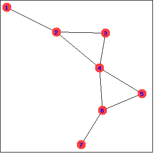 Categories: Package graphs · Package graphs - properties ·
- Function: bipartition (gr) 
Returns a bipartition of the vertices of the graph gr or an empty list if gr is not bipartite.
Example:
(%i1) load ("graphs")$ (%i2) h : heawood_graph()$ (%i3) [A,B]:bipartition(h); (%o3) [[8, 12, 6, 10, 0, 2, 4], [13, 5, 11, 7, 9, 1, 3]] (%i4) draw_graph(h, show_vertices=A, program=circular)$ Categories: Package graphs · Package graphs - properties ·
- Function: chromatic_index (gr) 
Returns the chromatic index of the graph gr.
Example:
(%i1) load ("graphs")$ (%i2) p : petersen_graph()$ (%i3) chromatic_index(p); (%o3) 4Categories: Package graphs · Package graphs - properties ·
- Function: chromatic_number (gr) 
Returns the chromatic number of the graph gr.
Example:
(%i1) load ("graphs")$ (%i2) chromatic_number(cycle_graph(5)); (%o2) 3 (%i3) chromatic_number(cycle_graph(6)); (%o3) 2Categories: Package graphs · Package graphs - properties ·
- Function: clear_edge_weight (e, gr) 
Removes the weight of the edge e in the graph gr.
Example:
(%i1) load ("graphs")$ (%i2) g : create_graph(3, [[[0,1], 1.5], [[1,2], 1.3]])$ (%i3) get_edge_weight([0,1], g); (%o3) 1.5 (%i4) clear_edge_weight([0,1], g)$ (%i5) get_edge_weight([0,1], g); (%o5) 1Categories: Package graphs · Package graphs - properties ·
- Function: clear_vertex_label (v, gr) 
Removes the label of the vertex v in the graph gr.
Example:
(%i1) load ("graphs")$ (%i2) g : create_graph([[0,"Zero"], [1, "One"]], [[0,1]])$ (%i3) get_vertex_label(0, g); (%o3) Zero (%i4) clear_vertex_label(0, g); (%o4) done (%i5) get_vertex_label(0, g); (%o5) falseCategories: Package graphs · Package graphs - properties ·
- Function: connected_components (gr) 
Returns the (vertex sets of) connected components of the graph gr.
Example:
(%i1) load ("graphs")$ (%i2) g: graph_union(cycle_graph(5), path_graph(4))$ (%i3) connected_components(g); (%o3) [[1, 2, 3, 4, 0], [8, 7, 6, 5]]Categories: Package graphs · Package graphs - properties ·
- Function: diameter (gr) 
Returns the diameter of the graph gr.
Example:
(%i1) load ("graphs")$ (%i2) diameter(dodecahedron_graph()); (%o2) 5Categories: Package graphs · Package graphs - properties ·
- Function: edge_coloring (gr) 
Returns an optimal coloring of the edges of the graph gr.
The function returns the chromatic index and a list representing the coloring of the edges of gr.
Example:
(%i1) load ("graphs")$ (%i2) p : petersen_graph()$ (%i3) [ch_index, col] : edge_coloring(p); (%o3) [4, [[[0, 5], 3], [[5, 7], 1], [[0, 1], 1], [[1, 6], 2], [[6, 8], 1], [[1, 2], 3], [[2, 7], 4], [[7, 9], 2], [[2, 3], 2], [[3, 8], 3], [[5, 8], 2], [[3, 4], 1], [[4, 9], 4], [[6, 9], 3], [[0, 4], 2]]] (%i4) assoc([0,1], col); (%o4) 1 (%i5) assoc([0,5], col); (%o5) 3Categories: Package graphs · Package graphs - properties ·
- Function: degree_sequence (gr) 
Returns the list of vertex degrees of the graph gr.
Example:
(%i1) load ("graphs")$ (%i2) degree_sequence(random_graph(10, 0.4)); (%o2) [2, 2, 2, 2, 2, 2, 3, 3, 3, 3]Categories: Package graphs · Package graphs - properties ·
- Function: edge_connectivity (gr) 
Returns the edge-connectivity of the graph gr.
See also
min_edge_cut.Categories: Package graphs · Package graphs - properties ·
- Function: edges (gr) 
Returns the list of edges (arcs) in a (directed) graph gr.
Example:
(%i1) load ("graphs")$ (%i2) edges(complete_graph(4)); (%o2) [[2, 3], [1, 3], [1, 2], [0, 3], [0, 2], [0, 1]]Categories: Package graphs · Package graphs - properties ·
- Function: get_edge_weight
get_edge_weight (e, gr)
get_edge_weight (e, gr, ifnot) ¶ -
Returns the weight of the edge e in the graph gr.
If there is no weight assigned to the edge, the function returns 1. If the edge is not present in the graph, the function signals an error or returns the optional argument ifnot.
Example:
(%i1) load ("graphs")$ (%i2) c5 : cycle_graph(5)$ (%i3) get_edge_weight([1,2], c5); (%o3) 1 (%i4) set_edge_weight([1,2], 2.0, c5); (%o4) done (%i5) get_edge_weight([1,2], c5); (%o5) 2.0Categories: Package graphs · Package graphs - properties ·
- Function: get_vertex_label (v, gr) 
Returns the label of the vertex v in the graph gr.
If no label is assigned to vertex v,
get_vertex_labelreturnsfalse.Example:
(%i1) load("graphs")$ (%i2) g: create_graph([[0, "Zero"], [1, "One"], 2, 3], [])$ (%i3) get_vertex_label(0, g); (%o3) Zero (%i4) get_vertex_label(2, g); (%o4) falseCategories: Package graphs · Package graphs - properties ·
- Function: get_unique_vertex_by_label (l, gr) 
Returns the unique vertex which has the label l in graph gr.
If there is no such vertex,
get_unique_vertex_by_labelreturnsfalse.If there are two or more vertices with label l,
get_unique_vertex_by_labelreports an error.Example:
(%i1) load ("graphs")$ (%i2) g: create_graph ([[0, "Zero"], [1, "One"], [2, "Other"], [3, "Other"]], []) $ (%i3) get_unique_vertex_by_label ("Zero", g); (%o3) 0 (%i4) get_unique_vertex_by_label ("Two", g); (%o4) false (%i5) errcatch (get_unique_vertex_by_label ("Other", g)); get_unique_vertex_by_label: two or more vertices have the same label "Other" (%o5) []Categories: Package graphs · Package graphs - properties ·
- Function: get_all_vertices_by_label (l, gr) 
Returns all vertices, if any, which have the label l in graph gr.
If there are no such vertices,
get_all_vertices_by_labelreturns an empty list[].Example:
(%i1) load ("graphs")$ (%i2) g: create_graph ([[0, "Zero"], [1, "One"], [2, "Other"], [3, "Other"]], []) $ (%i3) get_all_vertices_by_label ("Zero", g); (%o3) [0] (%i4) get_all_vertices_by_label ("Two", g); (%o4) [] (%i5) get_all_vertices_by_label ("Other", g); (%o5) [2, 3]Categories: Package graphs · Package graphs - properties ·
- Function: graph_charpoly (gr, x) 
Returns the characteristic polynomial (in variable x) of the graph gr.
Example:
(%i1) load ("graphs")$ (%i2) p : petersen_graph()$ (%i3) graph_charpoly(p, x), factor; 5 4 (%o3) (x - 3) (x - 1) (x + 2)Categories: Package graphs · Package graphs - properties ·
- Function: graph_center (gr) 
Returns the center of the graph gr.
Example:
(%i1) load ("graphs")$ (%i2) g : grid_graph(5,5)$ (%i3) graph_center(g); (%o3) [12]Categories: Package graphs · Package graphs - properties ·
- Function: graph_eigenvalues (gr) 
Returns the eigenvalues of the graph gr. The function returns eigenvalues in the same format as maxima
eigenvaluesfunction.Example:
(%i1) load ("graphs")$ (%i2) p : petersen_graph()$ (%i3) graph_eigenvalues(p); (%o3) [[3, - 2, 1], [1, 4, 5]]Categories: Package graphs · Package graphs - properties ·
- Function: graph_periphery (gr) 
Returns the periphery of the graph gr.
Example:
(%i1) load ("graphs")$ (%i2) g : grid_graph(5,5)$ (%i3) graph_periphery(g); (%o3) [24, 20, 4, 0]Categories: Package graphs · Package graphs - properties ·
- Function: graph_size (gr) 
Returns the number of edges in the graph gr.
Example:
(%i1) load ("graphs")$ (%i2) p : petersen_graph()$ (%i3) graph_size(p); (%o3) 15Categories: Package graphs · Package graphs - properties ·
- Function: graph_order (gr) 
Returns the number of vertices in the graph gr.
Example:
(%i1) load ("graphs")$ (%i2) p : petersen_graph()$ (%i3) graph_order(p); (%o3) 10Categories: Package graphs · Package graphs - properties ·
- Function: girth (gr) 
Returns the length of the shortest cycle in gr.
Example:
(%i1) load ("graphs")$ (%i2) g : heawood_graph()$ (%i3) girth(g); (%o3) 6Categories: Package graphs · Package graphs - properties ·
- Function: hamilton_cycle (gr) 
Returns the Hamilton cycle of the graph gr or an empty list if gr is not hamiltonian.
Example:
(%i1) load ("graphs")$ (%i2) c : cube_graph(3)$ (%i3) hc : hamilton_cycle(c); (%o3) [7, 3, 2, 6, 4, 0, 1, 5, 7] (%i4) draw_graph(c, show_edges=vertices_to_cycle(hc))$ Categories: Package graphs · Package graphs - properties ·
- Function: hamilton_path (gr) 
Returns the Hamilton path of the graph gr or an empty list if gr does not have a Hamilton path.
Example:
(%i1) load ("graphs")$ (%i2) p : petersen_graph()$ (%i3) hp : hamilton_path(p); (%o3) [0, 5, 7, 2, 1, 6, 8, 3, 4, 9] (%i4) draw_graph(p, show_edges=vertices_to_path(hp))$ Categories: Package graphs · Package graphs - properties ·
- Function: isomorphism (gr1, gr2) 
-
Returns a an isomorphism between graphs/digraphs gr1 and gr2. If gr1 and gr2 are not isomorphic, it returns an empty list.
Example:
(%i1) load ("graphs")$ (%i2) clk5:complement_graph(line_graph(complete_graph(5)))$ (%i3) isomorphism(clk5, petersen_graph()); (%o3) [9 -> 0, 2 -> 1, 6 -> 2, 5 -> 3, 0 -> 4, 1 -> 5, 3 -> 6, 4 -> 7, 7 -> 8, 8 -> 9]Categories: Package graphs · Package graphs - properties ·
- Function: in_neighbors (v, gr) 
Returns the list of in-neighbors of the vertex v in the directed graph gr.
Example:
(%i1) load ("graphs")$ (%i2) p : path_digraph(3)$ (%i3) in_neighbors(2, p); (%o3) [1] (%i4) out_neighbors(2, p); (%o4) []Categories: Package graphs · Package graphs - properties ·
- Function: is_biconnected (gr) 
Returns
trueif gr is 2-connected andfalseotherwise.Example:
(%i1) load ("graphs")$ (%i2) is_biconnected(cycle_graph(5)); (%o2) true (%i3) is_biconnected(path_graph(5)); (%o3) falseCategories: Package graphs · Package graphs - properties ·
- Function: is_bipartite (gr) 
Returns
trueif gr is bipartite (2-colorable) andfalseotherwise.Example:
(%i1) load ("graphs")$ (%i2) is_bipartite(petersen_graph()); (%o2) false (%i3) is_bipartite(heawood_graph()); (%o3) trueCategories: Package graphs · Package graphs - properties ·
- Function: is_connected (gr) 
Returns
trueif the graph gr is connected andfalseotherwise.Example:
(%i1) load ("graphs")$ (%i2) is_connected(graph_union(cycle_graph(4), path_graph(3))); (%o2) falseCategories: Package graphs · Package graphs - properties ·
- Function: is_digraph (gr) 
Returns
trueif gr is a directed graph andfalseotherwise.Example:
(%i1) load ("graphs")$ (%i2) is_digraph(path_graph(5)); (%o2) false (%i3) is_digraph(path_digraph(5)); (%o3) trueCategories: Package graphs · Package graphs - properties ·
- Function: is_edge_in_graph (e, gr) 
Returns
trueif e is an edge (arc) in the (directed) graph g andfalseotherwise.Example:
(%i1) load ("graphs")$ (%i2) c4 : cycle_graph(4)$ (%i3) is_edge_in_graph([2,3], c4); (%o3) true (%i4) is_edge_in_graph([3,2], c4); (%o4) true (%i5) is_edge_in_graph([2,4], c4); (%o5) false (%i6) is_edge_in_graph([3,2], cycle_digraph(4)); (%o6) falseCategories: Package graphs · Package graphs - properties ·
- Function: is_graph (gr) 
Returns
trueif gr is a graph andfalseotherwise.Example:
(%i1) load ("graphs")$ (%i2) is_graph(path_graph(5)); (%o2) true (%i3) is_graph(path_digraph(5)); (%o3) falseCategories: Package graphs · Package graphs - properties ·
- Function: is_graph_or_digraph (gr) 
Returns
trueif gr is a graph or a directed graph andfalseotherwise.Example:
(%i1) load ("graphs")$ (%i2) is_graph_or_digraph(path_graph(5)); (%o2) true (%i3) is_graph_or_digraph(path_digraph(5)); (%o3) trueCategories: Package graphs · Package graphs - properties ·
- Function: is_isomorphic (gr1, gr2) 
-
Returns
trueif graphs/digraphs gr1 and gr2 are isomorphic andfalseotherwise.See also
isomorphism.Example:
(%i1) load ("graphs")$ (%i2) clk5:complement_graph(line_graph(complete_graph(5)))$ (%i3) is_isomorphic(clk5, petersen_graph()); (%o3) trueCategories: Package graphs · Package graphs - properties ·
- Function: is_planar (gr) 
-
Returns
trueif gr is a planar graph andfalseotherwise.The algorithm used is the Demoucron’s algorithm, which is a quadratic time algorithm.
Example:
(%i1) load ("graphs")$ (%i2) is_planar(dodecahedron_graph()); (%o2) true (%i3) is_planar(petersen_graph()); (%o3) false (%i4) is_planar(petersen_graph(10,2)); (%o4) trueCategories: Package graphs · Package graphs - properties ·
- Function: is_sconnected (gr) 
Returns
trueif the directed graph gr is strongly connected andfalseotherwise.Example:
(%i1) load ("graphs")$ (%i2) is_sconnected(cycle_digraph(5)); (%o2) true (%i3) is_sconnected(path_digraph(5)); (%o3) falseCategories: Package graphs · Package graphs - properties ·
- Function: is_vertex_in_graph (v, gr) 
Returns
trueif v is a vertex in the graph g andfalseotherwise.Example:
(%i1) load ("graphs")$ (%i2) c4 : cycle_graph(4)$ (%i3) is_vertex_in_graph(0, c4); (%o3) true (%i4) is_vertex_in_graph(6, c4); (%o4) falseCategories: Package graphs · Package graphs - properties ·
- Function: is_tree (gr) 
Returns
trueif gr is a tree andfalseotherwise.Example:
(%i1) load ("graphs")$ (%i2) is_tree(random_tree(4)); (%o2) true (%i3) is_tree(graph_union(random_tree(4), random_tree(5))); (%o3) falseCategories: Package graphs · Package graphs - properties ·
- Function: laplacian_matrix (gr) 
Returns the laplacian matrix of the graph gr.
Example:
(%i1) load ("graphs")$ (%i2) laplacian_matrix(cycle_graph(5)); [ 2 - 1 0 0 - 1 ] [ ] [ - 1 2 - 1 0 0 ] [ ] (%o2) [ 0 - 1 2 - 1 0 ] [ ] [ 0 0 - 1 2 - 1 ] [ ] [ - 1 0 0 - 1 2 ]Categories: Package graphs · Package graphs - properties ·
- Function: max_clique (gr) 
Returns a maximum clique of the graph gr.
Example:
(%i1) load ("graphs")$ (%i2) g : random_graph(100, 0.5)$ (%i3) max_clique(g); (%o3) [6, 12, 31, 36, 52, 59, 62, 63, 80]Categories: Package graphs · Package graphs - properties ·
- Function: max_degree (gr) 
Returns the maximal degree of vertices of the graph gr and a vertex of maximal degree.
Example:
(%i1) load ("graphs")$ (%i2) g : random_graph(100, 0.02)$ (%i3) max_degree(g); (%o3) [6, 79] (%i4) vertex_degree(95, g); (%o4) 2Categories: Package graphs · Package graphs - properties ·
- Function: max_flow (net, s, t) 
Returns a maximum flow through the network net with the source s and the sink t.
The function returns the value of the maximal flow and a list representing the weights of the arcs in the optimal flow.
Example:
(%i1) load ("graphs")$ (%i2) net : create_graph( [1,2,3,4,5,6], [[[1,2], 1.0], [[1,3], 0.3], [[2,4], 0.2], [[2,5], 0.3], [[3,4], 0.1], [[3,5], 0.1], [[4,6], 1.0], [[5,6], 1.0]], directed=true)$ (%i3) [flow_value, flow] : max_flow(net, 1, 6); (%o3) [0.7, [[[1, 2], 0.5], [[1, 3], 0.2], [[2, 4], 0.2], [[2, 5], 0.3], [[3, 4], 0.1], [[3, 5], 0.1], [[4, 6], 0.3], [[5, 6], 0.4]]] (%i4) fl : 0$ (%i5) for u in out_neighbors(1, net) do fl : fl + assoc([1, u], flow)$ (%i6) fl; (%o6) 0.7Categories: Package graphs · Package graphs - properties ·
- Function: max_independent_set (gr) 
Returns a maximum independent set of the graph gr.
Example:
(%i1) load ("graphs")$ (%i2) d : dodecahedron_graph()$ (%i3) mi : max_independent_set(d); (%o3) [0, 3, 5, 9, 10, 11, 18, 19] (%i4) draw_graph(d, show_vertices=mi)$ Categories: Package graphs · Package graphs - properties ·
- Function: max_matching (gr) 
Returns a maximum matching of the graph gr.
Example:
(%i1) load ("graphs")$ (%i2) d : dodecahedron_graph()$ (%i3) m : max_matching(d); (%o3) [[5, 7], [8, 9], [6, 10], [14, 19], [13, 18], [12, 17], [11, 16], [0, 15], [3, 4], [1, 2]] (%i4) draw_graph(d, show_edges=m)$ Categories: Package graphs · Package graphs - properties ·
- Function: min_degree (gr) 
Returns the minimum degree of vertices of the graph gr and a vertex of minimum degree.
Example:
(%i1) load ("graphs")$ (%i2) g : random_graph(100, 0.1)$ (%i3) min_degree(g); (%o3) [3, 49] (%i4) vertex_degree(21, g); (%o4) 9Categories: Package graphs · Package graphs - properties ·
- Function: min_edge_cut (gr) 
Returns the minimum edge cut in the graph gr.
See also
edge_connectivity.Categories: Package graphs · Package graphs - properties ·
- Function: min_vertex_cover (gr) 
Returns the minimum vertex cover of the graph gr.
Categories: Package graphs · Package graphs - properties ·
- Function: min_vertex_cut (gr) 
Returns the minimum vertex cut in the graph gr.
See also
vertex_connectivity.Categories: Package graphs · Package graphs - properties ·
- Function: minimum_spanning_tree (gr) 
Returns the minimum spanning tree of the graph gr.
Example:
(%i1) load ("graphs")$ (%i2) g : graph_product(path_graph(10), path_graph(10))$ (%i3) t : minimum_spanning_tree(g)$ (%i4) draw_graph(g, show_edges=edges(t))$ Categories: Package graphs · Package graphs - properties ·
- Function: neighbors (v, gr) 
Returns the list of neighbors of the vertex v in the graph gr.
Example:
(%i1) load ("graphs")$ (%i2) p : petersen_graph()$ (%i3) neighbors(3, p); (%o3) [4, 8, 2]Categories: Package graphs · Package graphs - properties ·
- Function: odd_girth (gr) 
Returns the length of the shortest odd cycle in the graph gr.
Example:
(%i1) load ("graphs")$ (%i2) g : graph_product(cycle_graph(4), cycle_graph(7))$ (%i3) girth(g); (%o3) 4 (%i4) odd_girth(g); (%o4) 7Categories: Package graphs · Package graphs - properties ·
- Function: out_neighbors (v, gr) 
Returns the list of out-neighbors of the vertex v in the directed graph gr.
Example:
(%i1) load ("graphs")$ (%i2) p : path_digraph(3)$ (%i3) in_neighbors(2, p); (%o3) [1] (%i4) out_neighbors(2, p); (%o4) []Categories: Package graphs · Package graphs - properties ·
- Function: planar_embedding (gr) 
-
Returns the list of facial walks in a planar embedding of gr and
falseif gr is not a planar graph.The graph gr must be biconnected.
The algorithm used is the Demoucron’s algorithm, which is a quadratic time algorithm.
Example:
(%i1) load ("graphs")$ (%i2) planar_embedding(grid_graph(3,3)); (%o2) [[3, 6, 7, 8, 5, 2, 1, 0], [4, 3, 0, 1], [3, 4, 7, 6], [8, 7, 4, 5], [1, 2, 5, 4]]Categories: Package graphs · Package graphs - properties ·
- Function: print_graph (gr) 
Prints some information about the graph gr.
Example:
(%i1) load ("graphs")$ (%i2) c5 : cycle_graph(5)$ (%i3) print_graph(c5)$ Graph on 5 vertices with 5 edges. Adjacencies: 4 : 0 3 3 : 4 2 2 : 3 1 1 : 2 0 0 : 4 1 (%i4) dc5 : cycle_digraph(5)$ (%i5) print_graph(dc5)$ Digraph on 5 vertices with 5 arcs. Adjacencies: 4 : 0 3 : 4 2 : 3 1 : 2 0 : 1 (%i6) out_neighbors(0, dc5); (%o6) [1]Categories: Package graphs ·
- Function: radius (gr) 
Returns the radius of the graph gr.
Example:
(%i1) load ("graphs")$ (%i2) radius(dodecahedron_graph()); (%o2) 5Categories: Package graphs · Package graphs - properties ·
- Function: set_edge_weight (e, w, gr) 
Assigns the weight w to the edge e in the graph gr.
Example:
(%i1) load ("graphs")$ (%i2) g : create_graph([1, 2], [[[1,2], 1.2]])$ (%i3) get_edge_weight([1,2], g); (%o3) 1.2 (%i4) set_edge_weight([1,2], 2.1, g); (%o4) done (%i5) get_edge_weight([1,2], g); (%o5) 2.1Categories: Package graphs · Package graphs - properties ·
- Function: set_vertex_label (v, l, gr) 
Assigns the label l to the vertex v in the graph gr.
A label may be any Maxima expression, and two or more vertices may have the same label.
Example:
(%i1) load ("graphs")$ (%i2) g : create_graph([[1, "One"], [2, "Two"]], [[1, 2]])$ (%i3) get_vertex_label(1, g); (%o3) One (%i4) set_vertex_label(1, "oNE", g); (%o4) done (%i5) get_vertex_label(1, g); (%o5) oNE (%i6) h : create_graph([[11, x], [22, y], [33, x + y]], [[11, 33], [22, 33]]) $ (%i7) get_vertex_label (33, h); (%o7) y + xCategories: Package graphs · Package graphs - properties ·
- Function: shortest_path (u, v, gr) 
Returns the shortest path from u to v in the graph gr.
Example:
(%i1) load ("graphs")$ (%i2) d : dodecahedron_graph()$ (%i3) path : shortest_path(0, 7, d); (%o3) [0, 1, 19, 13, 7] (%i4) draw_graph(d, show_edges=vertices_to_path(path))$ Categories: Package graphs · Package graphs - properties ·
- Function: shortest_weighted_path (u, v, gr) 
Returns the length of the shortest weighted path and the shortest weighted path from u to v in the graph gr.
The length of a weighted path is the sum of edge weights of edges in the path. If an edge has no weight, then it has a default weight 1.
Example:
(%i1) load ("graphs")$ (%i2) g: petersen_graph(20, 2)$ (%i3) for e in edges(g) do set_edge_weight(e, random(1.0), g)$ (%i4) shortest_weighted_path(0, 10, g); (%o4) [2.575143920268482, [0, 20, 38, 36, 34, 32, 30, 10]]Categories: Package graphs · Package graphs - properties ·
- Function: strong_components (gr) 
Returns the strong components of a directed graph gr.
Example:
(%i1) load ("graphs")$ (%i2) t : random_tournament(4)$ (%i3) strong_components(t); (%o3) [[1], [0], [2], [3]] (%i4) vertex_out_degree(3, t); (%o4) 3Categories: Package graphs · Package graphs - properties ·
- Function: topological_sort (dag) 
-
Returns a topological sorting of the vertices of a directed graph dag or an empty list if dag is not a directed acyclic graph.
Example:
(%i1) load ("graphs")$ (%i2) g:create_graph( [1,2,3,4,5], [ [1,2], [2,5], [5,3], [5,4], [3,4], [1,3] ], directed=true)$ (%i3) topological_sort(g); (%o3) [1, 2, 5, 3, 4]Categories: Package graphs · Package graphs - properties ·
- Function: vertex_connectivity (g) 
Returns the vertex connectivity of the graph g.
See also
min_vertex_cut.Categories: Package graphs · Package graphs - properties ·
- Function: vertex_degree (v, gr) 
Returns the degree of the vertex v in the graph gr.
Categories: Package graphs · Package graphs - properties ·
- Function: vertex_distance (u, v, gr) 
Returns the length of the shortest path between u and v in the (directed) graph gr.
Example:
(%i1) load ("graphs")$ (%i2) d : dodecahedron_graph()$ (%i3) vertex_distance(0, 7, d); (%o3) 4 (%i4) shortest_path(0, 7, d); (%o4) [0, 1, 19, 13, 7]Categories: Package graphs · Package graphs - properties ·
- Function: vertex_eccentricity (v, gr) 
-
Returns the eccentricity of the vertex v in the graph gr.
Example:
(%i1) load ("graphs")$ (%i2) g:cycle_graph(7)$ (%i3) vertex_eccentricity(0, g); (%o3) 3Categories: Package graphs · Package graphs - properties ·
- Function: vertex_in_degree (v, gr) 
Returns the in-degree of the vertex v in the directed graph gr.
Example:
(%i1) load ("graphs")$ (%i2) p5 : path_digraph(5)$ (%i3) print_graph(p5)$ Digraph on 5 vertices with 4 arcs. Adjacencies: 4 : 3 : 4 2 : 3 1 : 2 0 : 1 (%i4) vertex_in_degree(4, p5); (%o4) 1 (%i5) in_neighbors(4, p5); (%o5) [3]Categories: Package graphs · Package graphs - properties ·
- Function: vertex_out_degree (v, gr) 
Returns the out-degree of the vertex v in the directed graph gr.
Example:
(%i1) load ("graphs")$ (%i2) t : random_tournament(10)$ (%i3) vertex_out_degree(0, t); (%o3) 2 (%i4) out_neighbors(0, t); (%o4) [7, 1]Categories: Package graphs · Package graphs - properties ·
- Function: vertices (gr) 
Returns the list of vertices in the graph gr.
Example:
(%i1) load ("graphs")$ (%i2) vertices(complete_graph(4)); (%o2) [3, 2, 1, 0]Categories: Package graphs · Package graphs - properties ·
- Function: vertex_coloring (gr) 
Returns an optimal coloring of the vertices of the graph gr.
The function returns the chromatic number and a list representing the coloring of the vertices of gr.
Example:
(%i1) load ("graphs")$ (%i2) p:petersen_graph()$ (%i3) vertex_coloring(p); (%o3) [3, [[0, 2], [1, 3], [2, 2], [3, 3], [4, 1], [5, 3], [6, 1], [7, 1], [8, 2], [9, 2]]]Categories: Package graphs · Package graphs - properties ·
- Function: wiener_index (gr) 
Returns the Wiener index of the graph gr.
Example:
(%i2) wiener_index(dodecahedron_graph()); (%o2) 500
Categories: Package graphs · Package graphs - properties ·
66.2.3 Modifying graphs
- Function: add_edge (e, gr) 
Adds the edge e to the graph gr.
Example:
(%i1) load ("graphs")$ (%i2) p : path_graph(4)$ (%i3) neighbors(0, p); (%o3) [1] (%i4) add_edge([0,3], p); (%o4) done (%i5) neighbors(0, p); (%o5) [3, 1]Categories: Package graphs · Package graphs - modifications ·
- Function: add_edges (e_list, gr) 
Adds all edges in the list e_list to the graph gr.
Example:
(%i1) load ("graphs")$ (%i2) g : empty_graph(3)$ (%i3) add_edges([[0,1],[1,2]], g)$ (%i4) print_graph(g)$ Graph on 3 vertices with 2 edges. Adjacencies: 2 : 1 1 : 2 0 0 : 1Categories: Package graphs · Package graphs - modifications ·
- Function: add_vertex (v, gr) 
Adds the vertex v to the graph gr.
Example:
(%i1) load ("graphs")$ (%i2) g : path_graph(2)$ (%i3) add_vertex(2, g)$ (%i4) print_graph(g)$ Graph on 3 vertices with 1 edges. Adjacencies: 2 : 1 : 0 0 : 1Categories: Package graphs · Package graphs - modifications ·
- Function: add_vertices (v_list, gr) 
Adds all vertices in the list v_list to the graph gr. A vertex may be any integer, and v_list may contain vertices in any order.
Categories: Package graphs · Package graphs - modifications ·
- Function: connect_vertices (v_list, u_list, gr) 
Connects all vertices from the list v_list with the vertices in the list u_list in the graph gr.
v_list and u_list can be single vertices or lists of vertices.
Example:
(%i1) load ("graphs")$ (%i2) g : empty_graph(4)$ (%i3) connect_vertices(0, [1,2,3], g)$ (%i4) print_graph(g)$ Graph on 4 vertices with 3 edges. Adjacencies: 3 : 0 2 : 0 1 : 0 0 : 3 2 1Categories: Package graphs · Package graphs - modifications ·
- Function: contract_edge (e, gr) 
Contracts the edge e in the graph gr.
Example:
(%i1) load ("graphs")$ (%i2) g: create_graph( 8, [[0,3],[1,3],[2,3],[3,4],[4,5],[4,6],[4,7]])$ (%i3) print_graph(g)$ Graph on 8 vertices with 7 edges. Adjacencies: 7 : 4 6 : 4 5 : 4 4 : 7 6 5 3 3 : 4 2 1 0 2 : 3 1 : 3 0 : 3 (%i4) contract_edge([3,4], g)$ (%i5) print_graph(g)$ Graph on 7 vertices with 6 edges. Adjacencies: 7 : 3 6 : 3 5 : 3 3 : 5 6 7 2 1 0 2 : 3 1 : 3 0 : 3Categories: Package graphs · Package graphs - modifications ·
- Function: remove_edge (e, gr) 
Removes the edge e from the graph gr.
Example:
(%i1) load ("graphs")$ (%i2) c3 : cycle_graph(3)$ (%i3) remove_edge([0,1], c3)$ (%i4) print_graph(c3)$ Graph on 3 vertices with 2 edges. Adjacencies: 2 : 0 1 1 : 2 0 : 2Categories: Package graphs · Package graphs - modifications ·
- Function: remove_vertex (v, gr) 
Removes the vertex v from the graph gr.
Categories: Package graphs ·
66.2.4 Reading and writing to files
- Function: dimacs_export
dimacs_export (gr, fl)
dimacs_export (gr, fl, comment1, ..., commentn) ¶ -
Exports the graph into the file fl in the DIMACS format. Optional comments will be added to the top of the file.
Categories: Package graphs · Package graphs - io ·
- Function: dimacs_import (fl) 
-
Returns the graph from file fl in the DIMACS format.
Categories: Package graphs · Package graphs - io ·
- Function: graph6_decode (str) 
-
Returns the graph encoded in the graph6 format in the string str.
Categories: Package graphs · Package graphs - io ·
- Function: graph6_encode (gr) 
-
Returns a string which encodes the graph gr in the graph6 format.
Categories: Package graphs · Package graphs - io ·
- Function: graph6_export (gr_list, fl) 
-
Exports graphs in the list gr_list to the file fl in the graph6 format.
Categories: Package graphs · Package graphs - io ·
- Function: graph6_import (fl) 
-
Returns a list of graphs from the file fl in the graph6 format.
Categories: Package graphs · Package graphs - io ·
- Function: sparse6_decode (str) 
-
Returns the graph encoded in the sparse6 format in the string str.
Categories: Package graphs · Package graphs - io ·
- Function: sparse6_encode (gr) 
-
Returns a string which encodes the graph gr in the sparse6 format.
Categories: Package graphs · Package graphs - io ·
- Function: sparse6_export (gr_list, fl) 
-
Exports graphs in the list gr_list to the file fl in the sparse6 format.
Categories: Package graphs · Package graphs - io ·
- Function: sparse6_import (fl) 
-
Returns a list of graphs from the file fl in the sparse6 format.
Categories: Package graphs · Package graphs - io ·
66.2.5 Visualization
- Function: draw_graph
draw_graph (graph)
draw_graph (graph, option1, ..., optionk) ¶ -
Draws the graph using the Package draw package.
The algorithm used to position vertices is specified by the optional argument program. The default value is
program=spring_embedding. draw_graph can also use the graphviz programs for positioning vertices, but graphviz must be installed separately.Example 1:
(%i1) load ("graphs")$ (%i2) g:grid_graph(10,10)$ (%i3) m:max_matching(g)$ (%i4) draw_graph(g, spring_embedding_depth=100, show_edges=m, edge_type=dots, vertex_size=0)$
Example 2:
(%i1) load ("graphs")$ (%i2) g:create_graph(16, [ [0,1],[1,3],[2,3],[0,2],[3,4],[2,4], [5,6],[6,4],[4,7],[6,7],[7,8],[7,10],[7,11], [8,10],[11,10],[8,9],[11,12],[9,15],[12,13], [10,14],[15,14],[13,14] ])$ (%i3) t:minimum_spanning_tree(g)$ (%i4) draw_graph( g, show_edges=edges(t), show_edge_width=4, show_edge_color=green, vertex_type=filled_square, vertex_size=2 )$
Example 3:
(%i1) load ("graphs")$ (%i2) g:create_graph(16, [ [0,1],[1,3],[2,3],[0,2],[3,4],[2,4], [5,6],[6,4],[4,7],[6,7],[7,8],[7,10],[7,11], [8,10],[11,10],[8,9],[11,12],[9,15],[12,13], [10,14],[15,14],[13,14] ])$ (%i3) mi : max_independent_set(g)$ (%i4) draw_graph( g, show_vertices=mi, show_vertex_type=filled_up_triangle, show_vertex_size=2, edge_color=cyan, edge_width=3, show_id=true, text_color=brown )$
Example 4:
(%i1) load ("graphs")$ (%i2) net : create_graph( [0,1,2,3,4,5], [ [[0,1], 3], [[0,2], 2], [[1,3], 1], [[1,4], 3], [[2,3], 2], [[2,4], 2], [[4,5], 2], [[3,5], 2] ], directed=true )$ (%i3) draw_graph( net, show_weight=true, vertex_size=0, show_vertices=[0,5], show_vertex_type=filled_square, head_length=0.2, head_angle=10, edge_color="dark-green", text_color=blue )$
Example 5:
(%i1) load("graphs")$ (%i2) g: petersen_graph(20, 2); (%o2) GRAPH (%i3) draw_graph(g, redraw=true, program=planar_embedding); (%o3) done
Example 6:
(%i1) load("graphs")$ (%i2) t: tutte_graph(); (%o2) GRAPH (%i3) draw_graph(t, redraw=true, fixed_vertices=[1,2,3,4,5,6,7,8,9]); (%o3) done Categories: Package graphs ·
- Option variable: draw_graph_program 
Default value: spring_embedding
The default value for the program used to position vertices in
draw_graphprogram.Categories: Package graphs · Package graphs - draw_graphs options ·
- draw_graph option: show_id 
Default value: false
If true then ids of the vertices are displayed.
Categories: Package graphs · Package graphs - draw_graphs options ·
- draw_graph option: show_label 
Default value: false
If true then labels of the vertices are displayed.
Categories: Package graphs · Package graphs - draw_graphs options ·
- draw_graph option: label_alignment 
Default value: center
Determines how to align the labels/ids of the vertices. Can be
left,centerorright.Categories: Package graphs · Package graphs - draw_graphs options ·
- draw_graph option: show_weight 
Default value: false
If true then weights of the edges are displayed.
Categories: Package graphs · Package graphs - draw_graphs options ·
- draw_graph option: vertex_type 
Default value: circle
Defines how vertices are displayed. See the point_type option for the
drawpackage for possible values.Categories: Package graphs · Package graphs - draw_graphs options ·
- draw_graph option: vertex_size 
The size of vertices.
Categories: Package graphs · Package graphs - draw_graphs options ·
- draw_graph option: vertex_color 
The color used for displaying vertices.
Categories: Package graphs · Package graphs - draw_graphs options ·
- draw_graph option: show_vertices 
Default value: []
Display selected vertices in the using a different color.
Categories: Package graphs · Package graphs - draw_graphs options ·
- draw_graph option: show_vertex_type 
Defines how vertices specified in show_vertices are displayed. See the point_type option for the
drawpackage for possible values.Categories: Package graphs · Package graphs - draw_graphs options ·
- draw_graph option: show_vertex_size 
The size of vertices in show_vertices.
Categories: Package graphs · Package graphs - draw_graphs options ·
- draw_graph option: show_vertex_color 
The color used for displaying vertices in the show_vertices list.
Categories: Package graphs · Package graphs - draw_graphs options ·
- draw_graph option: vertex_partition 
Default value: []
A partition
[[v1,v2,...],...,[vk,...,vn]]of the vertices of the graph. The vertices of each list in the partition will be drawn in a different color.Categories: Package graphs · Package graphs - draw_graphs options ·
- draw_graph option: vertex_coloring 
Specifies coloring of the vertices. The coloring col must be specified in the format as returned by vertex_coloring.
Categories: Package graphs · Package graphs - draw_graphs options ·
- draw_graph option: edge_color 
The color used for displaying edges.
Categories: Package graphs · Package graphs - draw_graphs options ·
- draw_graph option: edge_width 
The width of edges.
Categories: Package graphs · Package graphs - draw_graphs options ·
- draw_graph option: edge_type 
Defines how edges are displayed. See the line_type option for the
drawpackage.Categories: Package graphs · Package graphs - draw_graphs options ·
- draw_graph option: show_edges 
Display edges specified in the list e_list using a different color.
Categories: Package graphs · Package graphs - draw_graphs options ·
- draw_graph option: show_edge_color 
The color used for displaying edges in the show_edges list.
Categories: Package graphs · Package graphs - draw_graphs options ·
- draw_graph option: show_edge_width 
The width of edges in show_edges.
Categories: Package graphs · Package graphs - draw_graphs options ·
- draw_graph option: show_edge_type 
Defines how edges in show_edges are displayed. See the line_type option for the
drawpackage.Categories: Package graphs · Package graphs - draw_graphs options ·
- draw_graph option: edge_partition 
A partition
[[e1,e2,...],...,[ek,...,em]]of edges of the graph. The edges of each list in the partition will be drawn using a different color.Categories: Package graphs · Package graphs - draw_graphs options ·
- draw_graph option: edge_coloring 
The coloring of edges. The coloring must be specified in the format as returned by the function edge_coloring.
Categories: Package graphs · Package graphs - draw_graphs options ·
- draw_graph option: redraw 
Default value: false
If
true, vertex positions are recomputed even if the positions have been saved from a previous drawing of the graph.Categories: Package graphs · Package graphs - draw_graphs options ·
- draw_graph option: head_angle 
Default value: 15
The angle for the arrows displayed on arcs (in directed graphs).
Categories: Package graphs · Package graphs - draw_graphs options ·
- draw_graph option: head_length 
Default value: 0.1
The length for the arrows displayed on arcs (in directed graphs).
Categories: Package graphs · Package graphs - draw_graphs options ·
- draw_graph option: spring_embedding_depth 
Default value: 50
The number of iterations in the spring embedding graph drawing algorithm.
Categories: Package graphs · Package graphs - draw_graphs options ·
- draw_graph option: terminal 
The terminal used for drawing (see the terminal option in the
drawpackage).Categories: Package graphs · Package graphs - draw_graphs options ·
- draw_graph option: file_name 
The filename of the drawing if terminal is not screen.
Categories: Package graphs · Package graphs - draw_graphs options ·
- draw_graph option: program 
Defines the program used for positioning vertices of the graph. Can be one of the graphviz programs (dot, neato, twopi, circ, fdp), circular, spring_embedding or planar_embedding. planar_embedding is only available for 2-connected planar graphs. When
program=spring_embedding, a set of vertices with fixed position can be specified with the fixed_vertices option.Categories: Package graphs · Package graphs - draw_graphs options ·
- draw_graph option: fixed_vertices 
Specifies a list of vertices which will have positions fixed along a regular polygon. Can be used when
program=spring_embedding.Categories: Package graphs · Package graphs - draw_graphs options ·
- Function: vertices_to_path (v_list) 
Converts a list v_list of vertices to a list of edges of the path defined by v_list.
Categories: Package graphs ·
- Function: vertices_to_cycle (v_list) 
Converts a list v_list of vertices to a list of edges of the cycle defined by v_list.
Categories: Package graphs ·
Next: Package hompack, Previous: Package graphs [Contents][Index]
67 Package grobner
67.1 Introduction to grobner
grobner is a package for working with Groebner bases in Maxima.
To use the following functions you must load the grobner.lisp package.
load("grobner");
A demo can be started by
demo("grobner.demo");
or
batch("grobner.demo")
Some of the calculation in the demo will take a lot of time therefore the output grobner-demo.output of the demo can be found in the same directory as the demo file.
67.1.1 Notes on the grobner package
The package was written by
Marek Rychlik
http://alamos.math.arizona.edu
and is released 2002-05-24 under the terms of the General Public License(GPL) (see file grobner.lisp). This documentation was extracted from the files
README, grobner.lisp, grobner.demo, grobner-demo.output
by Günter Nowak. Suggestions for improvement of the documentation can be discussed at the maxima-mailing-list maxima@math.utexas.edu. The code is a little bit out of date now. Modern implementation use the fast F4 algorithm described in
A new efficient algorithm for computing Gröbner bases (F4) Jean-Charles Faugère LIP6/CNRS Université Paris VI January 20, 1999
67.1.2 Implementations of admissible monomial orders in grobner
-
lexpure lexicographic, default order for monomial comparisons
-
grlextotal degree order, ties broken by lexicographic
-
grevlextotal degree, ties broken by reverse lexicographic
-
invlexinverse lexicographic order
Previous: Introduction to grobner [Contents][Index]
67.2 Functions and Variables for grobner
- Global switches for grobner
- Simple operators in grobner
- Other functions in grobner
- Standard postprocessing of Groebner Bases
67.2.1 Global switches for grobner
- Option variable: poly_monomial_order 
Default value:
lexThis global switch controls which monomial order is used in polynomial and Groebner Bases calculations. If not set,
lexwill be used.Categories: Package grobner ·
- Option variable: poly_coefficient_ring 
Default value:
expression_ringThis switch indicates the coefficient ring of the polynomials that will be used in grobner calculations. If not set, maxima’s general expression ring will be used. This variable may be set to
ring_of_integersif desired.Categories: Package grobner ·
- Option variable: poly_primary_elimination_order 
Default value:
falseName of the default order for eliminated variables in elimination-based functions. If not set,
lexwill be used.Categories: Package grobner ·
- Option variable: poly_secondary_elimination_order 
Default value:
falseName of the default order for kept variables in elimination-based functions. If not set,
lexwill be used.Categories: Package grobner ·
- Option variable: poly_elimination_order 
Default value:
falseName of the default elimination order used in elimination calculations. If set, it overrides the settings in variables
poly_primary_elimination_orderandpoly_secondary_elimination_order. The user must ensure that this is a true elimination order valid for the number of eliminated variables.Categories: Package grobner ·
- Option variable: poly_return_term_list 
Default value:
falseIf set to
true, all functions in this package will return each polynomial as a list of terms in the current monomial order rather than a maxima general expression.Categories: Package grobner ·
- Option variable: poly_grobner_debug 
Default value:
falseIf set to
true, produce debugging and tracing output.Categories: Package grobner ·
- Option variable: poly_grobner_algorithm 
Default value:
buchbergerPossible values:
-
buchberger -
parallel_buchberger -
gebauer_moeller
The name of the algorithm used to find the Groebner Bases.
Categories: Package grobner ·-
- Option variable: poly_top_reduction_only 
Default value:
falseIf not
false, use top reduction only whenever possible. Top reduction means that division algorithm stops after the first reduction.Categories: Package grobner ·
67.2.2 Simple operators in grobner
poly_add, poly_subtract, poly_multiply and poly_expt
are the arithmetical operations on polynomials.
These are performed using the internal representation, but the results are converted back to the
maxima general form.
- Function: poly_add (poly1, poly2, varlist) 
Adds two polynomials poly1 and poly2.
(%i1) poly_add(z+x^2*y,x-z,[x,y,z]); 2 (%o1) x y + xCategories: Package grobner ·
- Function: poly_subtract (poly1, poly2, varlist) 
Subtracts a polynomial poly2 from poly1.
(%i1) poly_subtract(z+x^2*y,x-z,[x,y,z]); 2 (%o1) 2 z + x y - xCategories: Package grobner ·
- Function: poly_multiply (poly1, poly2, varlist) 
Returns the product of polynomials poly1 and poly2.
(%i2) poly_multiply(z+x^2*y,x-z,[x,y,z])-(z+x^2*y)*(x-z),expand; (%o1) 0
Categories: Package grobner ·
- Function: poly_s_polynomial (poly1, poly2, varlist) 
Returns the syzygy polynomial (S-polynomial) of two polynomials poly1 and poly2.
Categories: Package grobner ·
- Function: poly_primitive_part (poly1, varlist) 
Returns the polynomial poly divided by the GCD of its coefficients.
(%i1) poly_primitive_part(35*y+21*x,[x,y]); (%o1) 5 y + 3 x
Categories: Package grobner ·
- Function: poly_normalize (poly, varlist) 
Returns the polynomial poly divided by the leading coefficient. It assumes that the division is possible, which may not always be the case in rings which are not fields.
Categories: Package grobner ·
67.2.3 Other functions in grobner
- Function: poly_expand (poly, varlist) 
This function parses polynomials to internal form and back. It is equivalent to
expand(poly)if poly parses correctly to a polynomial. If the representation is not compatible with a polynomial in variables varlist, the result is an error. It can be used to test whether an expression correctly parses to the internal representation. The following examples illustrate that indexed and transcendental function variables are allowed.(%i1) poly_expand((x-y)*(y+x),[x,y]); 2 2 (%o1) x - y (%i2) poly_expand((y+x)^2,[x,y]); 2 2 (%o2) y + 2 x y + x (%i3) poly_expand((y+x)^5,[x,y]); 5 4 2 3 3 2 4 5 (%o3) y + 5 x y + 10 x y + 10 x y + 5 x y + x (%i4) poly_expand(-1-x*exp(y)+x^2/sqrt(y),[x]); 2 y x (%o4) - x %e + ------- - 1 sqrt(y) (%i5) poly_expand(-1-sin(x)^2+sin(x),[sin(x)]); 2 (%o5) - sin (x) + sin(x) - 1Categories: Package grobner ·
- Function: poly_expt (poly, number, varlist) 
exponentitates poly by a positive integer number. If number is not a positive integer number an error will be raised.
(%i1) poly_expt(x-y,3,[x,y])-(x-y)^3,expand; (%o1) 0
Categories: Package grobner ·
- Function: poly_content (poly. varlist) 
poly_contentextracts the GCD of its coefficients(%i1) poly_content(35*y+21*x,[x,y]); (%o1) 7
Categories: Package grobner ·
- Function: poly_pseudo_divide (poly, polylist, varlist) 
Pseudo-divide a polynomial poly by the list of n polynomials polylist. Return multiple values. The first value is a list of quotients a. The second value is the remainder r. The third argument is a scalar coefficient c, such that c*poly can be divided by polylist within the ring of coefficients, which is not necessarily a field. Finally, the fourth value is an integer count of the number of reductions performed. The resulting objects satisfy the equation:
c*poly=sum(a[i]*polylist[i],i=1...n)+r.
Categories: Package grobner ·
- Function: poly_exact_divide (poly1, poly2, varlist) 
Divide a polynomial poly1 by another polynomial poly2. Assumes that exact division with no remainder is possible. Returns the quotient.
Categories: Package grobner ·
- Function: poly_normal_form (poly, polylist, varlist) 
poly_normal_formfinds the normal form of a polynomial poly with respect to a set of polynomials polylist.Categories: Package grobner ·
- Function: poly_buchberger_criterion (polylist, varlist) 
Returns
trueif polylist is a Groebner basis with respect to the current term order, by using the Buchberger criterion: for every two polynomials h1 and h2 in polylist the S-polynomial S(h1,h2) reduces to 0 modulo polylist.Categories: Package grobner ·
- Function: poly_buchberger (polylist_fl varlist) 
poly_buchbergerperforms the Buchberger algorithm on a list of polynomials and returns the resulting Groebner basis.Categories: Package grobner ·
67.2.4 Standard postprocessing of Groebner Bases
The k-th elimination Ideal I_k of an Ideal I over K[ x[1],...,x[n] ] is the ideal intersect(I, K[ x[k+1],...,x[n] ]).
The colon ideal I:J is the ideal {h|for all w in J: w*h in I}.
The ideal I:p^inf is the ideal {h| there is a n in N: p^n*h in I}.
The ideal I:J^inf is the ideal {h| there is a n in N and a p in J: p^n*h in I}.
The radical ideal sqrt(I) is the ideal {h| there is a n in N : h^n in I }.
- Function: poly_reduction (polylist, varlist) 
poly_reductionreduces a list of polynomials polylist, so that each polynomial is fully reduced with respect to the other polynomials.Categories: Package grobner ·
- Function: poly_minimization (polylist, varlist) 
Returns a sublist of the polynomial list polylist spanning the same monomial ideal as polylist but minimal, i.e. no leading monomial of a polynomial in the sublist divides the leading monomial of another polynomial.
Categories: Package grobner ·
- Function: poly_normalize_list (polylist, varlist) 
poly_normalize_listappliespoly_normalizeto each polynomial in the list. That means it divides every polynomial in a list polylist by its leading coefficient.Categories: Package grobner ·
- Function: poly_grobner (polylist, varlist) 
Returns a Groebner basis of the ideal span by the polynomials polylist. Affected by the global flags.
Categories: Package grobner ·
- Function: poly_reduced_grobner (polylist, varlist) 
Returns a reduced Groebner basis of the ideal span by the polynomials polylist. Affected by the global flags.
Categories: Package grobner ·
- Function: poly_depends_p (poly, var, varlist) 
poly_dependstests whether a polynomial depends on a variable var.Categories: Package grobner · Predicate functions ·
- Function: poly_elimination_ideal (polylist, number, varlist) 
-
poly_elimination_idealreturns the grobner basis of the number-th elimination ideal of an ideal specified as a list of generating polynomials (not necessarily Groebner basis).Categories: Package grobner ·
- Function: poly_colon_ideal (polylist1, polylist2, varlist) 
-
Returns the reduced Groebner basis of the colon ideal
I(polylist1):I(polylist2)
where polylist1 and polylist2 are two lists of polynomials.
Categories: Package grobner ·
- Function: poly_ideal_intersection (polylist1, polylist2, varlist) 
-
poly_ideal_intersectionreturns the intersection of two ideals.Categories: Package grobner ·
- Function: poly_lcm (poly1, poly2, varlist) 
Returns the lowest common multiple of poly1 and poly2.
Categories: Package grobner ·
- Function: poly_gcd (poly1, poly2, varlist) 
-
Returns the greatest common divisor of poly1 and poly2.
See also
ezgcd,gcd,gcdex, andgcdivide.Example:
(%i1) p1:6*x^3+19*x^2+19*x+6; 3 2 (%o1) 6 x + 19 x + 19 x + 6 (%i2) p2:6*x^5+13*x^4+12*x^3+13*x^2+6*x; 5 4 3 2 (%o2) 6 x + 13 x + 12 x + 13 x + 6 x (%i3) poly_gcd(p1, p2, [x]); 2 (%o3) 6 x + 13 x + 6Categories: Package grobner ·
- Function: poly_grobner_equal (polylist1, polylist2, varlist) 
poly_grobner_equaltests whether two Groebner Bases generate the same ideal. Returnstrueif two lists of polynomials polylist1 and polylist2, assumed to be Groebner Bases, generate the same ideal, andfalseotherwise. This is equivalent to checking that every polynomial of the first basis reduces to 0 modulo the second basis and vice versa. Note that in the example below the first list is not a Groebner basis, and thus the result isfalse.(%i1) poly_grobner_equal([y+x,x-y],[x,y],[x,y]); (%o1) false
Categories: Package grobner ·
- Function: poly_grobner_subsetp (polylist1, polylist2, varlist) 
-
poly_grobner_subsetptests whether an ideal generated by polylist1 is contained in the ideal generated by polylist2. For this test to always succeed, polylist2 must be a Groebner basis.Categories: Package grobner · Predicate functions ·
- Function: poly_grobner_member (poly, polylist, varlist) 
-
Returns
trueif a polynomial poly belongs to the ideal generated by the polynomial list polylist, which is assumed to be a Groebner basis. Returnsfalseotherwise.poly_grobner_membertests whether a polynomial belongs to an ideal generated by a list of polynomials, which is assumed to be a Groebner basis. Equivalent tonormal_formbeing 0.Categories: Package grobner ·
- Function: poly_ideal_saturation1 (polylist, poly, varlist) 
Returns the reduced Groebner basis of the saturation of the ideal
I(polylist):poly^inf
Geometrically, over an algebraically closed field, this is the set of polynomials in the ideal generated by polylist which do not identically vanish on the variety of poly.
Categories: Package grobner ·
- Function: poly_ideal_saturation (polylist1, polylist2, varlist) 
Returns the reduced Groebner basis of the saturation of the ideal
I(polylist1):I(polylist2)^inf
Geometrically, over an algebraically closed field, this is the set of polynomials in the ideal generated by polylist1 which do not identically vanish on the variety of polylist2.
Categories: Package grobner ·
- Function: poly_ideal_polysaturation1 (polylist1, polylist2, varlist) 
polylist2 is a list of n polynomials
[poly1,...,polyn]. Returns the reduced Groebner basis of the idealI(polylist):poly1^inf:...:polyn^inf
obtained by a sequence of successive saturations in the polynomials of the polynomial list polylist2 of the ideal generated by the polynomial list polylist1.
Categories: Package grobner ·
- Function: poly_ideal_polysaturation (polylist, polylistlist, varlist) 
polylistlist is a list of n list of polynomials
[polylist1,...,polylistn]. Returns the reduced Groebner basis of the saturation of the idealI(polylist):I(polylist_1)^inf:...:I(polylist_n)^inf
Categories: Package grobner ·
- Function: poly_saturation_extension (poly, polylist, varlist1, varlist2) 
-
poly_saturation_extensionimplements the famous Rabinowitz trick.Categories: Package grobner ·
- Function: poly_polysaturation_extension (poly, polylist, varlist1, varlist2) 
-
Categories: Package grobner ·
Next: Package impdiff, Previous: Package grobner [Contents][Index]
68 Package hompack
Next: Functions and Variables for hompack, Up: Package hompack [Contents][Index]
68.1 Introduction to hompack
Hompack is a Common Lisp translation (via f2cl) of the
Fortran library HOMPACK, as obtained from Netlib.
Previous: Introduction to hompack, Up: Package hompack [Contents][Index]
68.2 Functions and Variables for hompack
- Function: hompack_polsys (eqnlist, varlist [, iflg1, epsbig, epssml, numrr]) 
Finds the roots of the system of polynomials in the variables varlist in the system of equations in eqnlist. The number of equations must match number of variables. Each equation must be a polynomial with variables in varlist. The coefficients must be real numbers.
The optional keyword arguments provide some control over the algorithm.
epsbigis the local error tolerance allowed by the path tracker, defaulting to 1e-4.
epssmlis the accuracy desired for the final solution, defaulting to 1d-14.
numrris the number of multiples of 1000 steps that will be tried before abandoning a path, defaulting to 10.
iflg1defaulting to 0, controls the algorithm as follows:
0If the problem is to be solved without calling
polsys’ scaling routine,sclgnp, and without using the projective transformation.1If scaling but no projective transformation is to be used.
10If no scaling but projective transformation is to be used.
11If both scaling and projective transformation are to be used.
hompack_polsysreturns a list. The elements of the list are:retcodeIndicates whether the solution is valid or not.
0Solution found without problems
1Solution succeeded but
iflg2indicates some issues with a root. (That is,iflg2is not all ones.)-1NN, the declared dimension of the number of terms in the polynomials, is too small. (This should not happen.)-2MMAXT, the declared dimension for the internal coefficient and degree arrays, is too small. (This should not happen.)-3TTOTDG, the total degree of the equations, is too small. (This should not happen.)-4LENWK, the length of the internal real work array, is too small. (This should not happen.)-5LENIWK, the length of the internal integer work array, is too small. (This should not happen.)-6iflg1 is not 0 or 1, or 10 or 11. (This should not happen; an error should be thrown before
polsysis called.)
rootsThe roots of the system of equations. This is in the same format as
solvewould return.iflg2A list containing information on how the path for the m’th root terminated:
1Normal return
2Specified error tolerance cannot be met. Increase epsbig and epssml and rerun.
3Maximum number of steps exceeded. To track the path further, increase numrr and rerun the path. However, the path may be diverging, if the lambda value is near 1 and the roots values are large.
4Jacobian matrix does not have full rank. The algorithm has failed (the zero curve of the homotopy map cannot be followed any further).
5The tracking algorithm has lost the zero curve of the homotopy map and is not making progress. The error tolerances epsbig and epssml were too lenient. The problem should be restarted with smaller error tolerances.
6The normal flow newton iteration in
stepnforrootnffailed to converge. The error tolerance epsbig may be too stringent.7Illegal input parameters, a fatal error.
lambdaA list of the final lambda value for the m-th root, where lambda is the continuation parameter.
arclenA list of the arc length of the m-th root.
nfeA list of the number of jacobian matrix evaluations required to track the m-th root.
Here are some examples of using
hompack_polsys.(%i1) load(hompack)$
(%i2) hompack_polsys([x1^2-1, x2^2-2],[x1,x2]); (%o2) [0, [[x1 = 7.493410174972965e-17 %i - 1.0, x2 = - 2.1199276810167172e-16 %i - 1.4142135623730951], [x1 = 1.0 - 1.7812202259088373e-17 %i, x2 = - 9.892128000334418e-17 %i - 1.4142135623730951], [x1 = - 8.745710933584358e-17 %i - 1.0, x2 = 1.4142135623730951 - 3.1543521174128613e-17 %i], [x1 = 1.0 - 5.5487454344135625e-18 %i, x2 = 9.617653810456737e-17 %i + 1.4142135623730951]], [1, 1, 1, 1], [1.0, 1.0, 0.9999999999999999, 0.9999999999999999], [4.6126237693413445, 4.6126230108601, 4.612623872939582, 4.6126231144843475], [40, 40, 40, 40]]
The analytical solution can be obtained with solve:
(%i1) solve([x1^2-1, x2^2-2],[x1,x2]); (%o1) [[x1 = 1, x2 = - sqrt(2)], [x1 = 1, x2 = sqrt(2)], [x1 = - 1, x2 = - sqrt(2)], [x1 = - 1, x2 = sqrt(2)]]We see that
hompack_polsysreturned the correct answer except that the roots are in a different order and there is a small imaginary part.Another example, with corresponding solution from solve:
(%i1) load(hompack)$
(%i2) hompack_polsys([x1^2 + 2*x2^2 + x1*x2 - 5, 2*x1^2 + x2^2 + x2-4],[x1,x2]); (%o2) [0, [[x1 = 1.2015573017007832 - 6.51849608628558e-16 %i, x2 = - 2.2667444298167825e-16 %i - 1.6672703634801431], [x1 = - 5.901956169878514e-17 %i - 1.4285291895653132, x2 = - 6.670215053038164e-17 %i - 0.9106199083334114], [x1 = 1.942890293094024e-16 %i + 0.5920619420732687, x2 = 1.383859154368197 - 1.942890293094024e-16 %i], [x1 = 0.08945540033671631 - 8.534583737796769e-16 %i, x2 = 2.415141536592239e-16 %i + 1.5576674810817213]], [1, 1, 1, 1], [1.0000000000000004, 1.0000000000000002, 1.0, 0.9999999999999999], [6.205795654034981, 7.7222132593900525, 7.228287079174324, 5.6114742835849105], [35, 41, 48, 40]]
(%i3) solve([x1^2+2*x2^2+x1*x2 - 5, 2*x1^2+x2^2+x2-4],[x1,x2]); (%o3) [[x1 = 0.08945540336850383, x2 = 1.5576673866090713], [x1 = 0.5920619554695062, x2 = 1.3838592860838075], [x1 = 1.2015573525007488, x2 = - 1.66727025803531], [x1 = - 1.428529150636283, x2 = - 0.9106198942815954]]
Note that
hompack_polsyscan sometimes be very slow. Perhapssolvecan be used. Or perhapseliminatecan be used to convert the system of polynomials into one polynomial for whichallrootscan find all the roots.Categories: Package hompack ·
Next: Package interpol, Previous: Package hompack [Contents][Index]
69 Package impdiff
Previous: Package impdiff, Up: Package impdiff [Contents][Index]
69.1 Functions and Variables for impdiff
- Function: implicit_derivative (f,indvarlist,orderlist,depvar) 
This subroutine computes implicit derivatives of multivariable functions. f is an array function, the indexes are the derivative degree in the indvarlist order; indvarlist is the independent variable list; orderlist is the order desired; and depvar is the dependent variable.
To use this function write first
load("impdiff").
Next: Package itensor, Previous: Package impdiff [Contents][Index]
70 Package interpol
Next: Functions and Variables for interpol, Previous: Package interpol, Up: Package interpol [Contents][Index]
70.1 Introduction to interpol
Package interpol defines the Lagrangian, the linear and the cubic
splines methods for polynomial interpolation.
For comments, bugs or suggestions, please contact me at ’mario AT edu DOT xunta DOT es’.
Previous: Introduction to interpol, Up: Package interpol [Contents][Index]
70.2 Functions and Variables for interpol
- Function: lagrange
lagrange (points)
lagrange (points, option) ¶ -
Computes the polynomial interpolation by the Lagrangian method. Argument points must be either:
- a two column matrix,
p:matrix([2,4],[5,6],[9,3]), - a list of pairs,
p: [[2,4],[5,6],[9,3]], - a list of numbers,
p: [4,6,3], in which case the abscissas will be assigned automatically to 1, 2, 3, etc.
In the first two cases the pairs are ordered with respect to the first coordinate before making computations.
With the option argument it is possible to select the name for the independent variable, which is
'xby default; to define another one, write something likevarname='z.Note that when working with high degree polynomials, floating point evaluations are unstable.
See also
linearinterpol,cspline, andratinterpol.Examples:
(%i1) load("interpol")$ (%i2) p:[[7,2],[8,2],[1,5],[3,2],[6,7]]$ (%i3) lagrange(p); (x - 7) (x - 6) (x - 3) (x - 1) (%o3) ------------------------------- 35 (x - 8) (x - 6) (x - 3) (x - 1) - ------------------------------- 12 7 (x - 8) (x - 7) (x - 3) (x - 1) + --------------------------------- 30 (x - 8) (x - 7) (x - 6) (x - 1) - ------------------------------- 60 (x - 8) (x - 7) (x - 6) (x - 3) + ------------------------------- 84 (%i4) f(x):=''%; (x - 7) (x - 6) (x - 3) (x - 1) (%o4) f(x) := ------------------------------- 35 (x - 8) (x - 6) (x - 3) (x - 1) - ------------------------------- 12 7 (x - 8) (x - 7) (x - 3) (x - 1) + --------------------------------- 30 (x - 8) (x - 7) (x - 6) (x - 1) - ------------------------------- 60 (x - 8) (x - 7) (x - 6) (x - 3) + ------------------------------- 84 (%i5) /* Evaluate the polynomial at some points */ expand(map(f,[2.3,5/7,%pi])); 4 3 2 919062 73 %pi 701 %pi 8957 %pi (%o5) [- 1.567535, ------, ------- - -------- + --------- 84035 420 210 420 5288 %pi 186 - -------- + ---] 105 5 (%i6) %,numer; (%o6) [- 1.567535, 10.9366573451538, 2.89319655125692] (%i7) load("draw")$ /* load draw package */ (%i8) /* Plot the polynomial together with points */ draw2d( color = red, key = "Lagrange polynomial", explicit(f(x),x,0,10), point_size = 3, color = blue, key = "Sample points", points(p))$ (%i9) /* Change variable name */ lagrange(p, varname=w); (w - 7) (w - 6) (w - 3) (w - 1) (%o9) ------------------------------- 35 (w - 8) (w - 6) (w - 3) (w - 1) - ------------------------------- 12 7 (w - 8) (w - 7) (w - 3) (w - 1) + --------------------------------- 30 (w - 8) (w - 7) (w - 6) (w - 1) - ------------------------------- 60 (w - 8) (w - 7) (w - 6) (w - 3) + ------------------------------- 84Categories: Package interpol · - a two column matrix,
- Function: charfun2 (x, a, b) 
-
The characteristic or indicator function on the half-open interval [a, b), that is, including a and excluding b.
When x >= a and x < b evaluates to
trueorfalse,charfun2returns 1 or 0, respectively.Otherwise,
charfun2returns a partially-evaluated result in terms ofcharfun.Package
interpolloads this function.See also
charfun.Examples:
When x >= a and x < b evaluates to
trueorfalse,charfun2returns 1 or 0, respectively.(%i1) load ("interpol") $ (%i2) charfun2 (5, 0, 100); (%o2) 1 (%i3) charfun2 (-5, 0, 100); (%o3) 0Otherwise,
charfun2returns a partially-evaluated result in terms ofcharfun.(%i1) load ("interpol") $ (%i2) charfun2 (t, 0, 100); (%o2) charfun((0 <= t) and (t < 100)) (%i3) charfun2 (5, u, v); (%o3) charfun((u <= 5) and (5 < v)) (%i4) assume (v > u, u > 5); (%o4) [v > u, u > 5] (%i5) charfun2 (5, u, v); (%o5) 0Categories: Package interpol ·
- Function: linearinterpol
linearinterpol (points)
linearinterpol (points, option) ¶ -
Computes the polynomial interpolation by the linear method. Argument points must be either:
- a two column matrix,
p:matrix([2,4],[5,6],[9,3]), - a list of pairs,
p: [[2,4],[5,6],[9,3]], - a list of numbers,
p: [4,6,3], in which case the abscissas will be assigned automatically to 1, 2, 3, etc.
In the first two cases the pairs are ordered with respect to the first coordinate before making computations.
With the option argument it is possible to select the name for the independent variable, which is
'xby default; to define another one, write something likevarname='z.See also
lagrange,cspline, andratinterpol.Examples:
(%i1) load("interpol")$ (%i2) p: matrix([7,2],[8,3],[1,5],[3,2],[6,7])$ (%i3) linearinterpol(p); 13 3 x (%o3) (-- - ---) charfun2(x, minf, 3) 2 2 + (x - 5) charfun2(x, 7, inf) + (37 - 5 x) charfun2(x, 6, 7) 5 x + (--- - 3) charfun2(x, 3, 6) 3 (%i4) f(x):=''%; 13 3 x (%o4) f(x) := (-- - ---) charfun2(x, minf, 3) 2 2 + (x - 5) charfun2(x, 7, inf) + (37 - 5 x) charfun2(x, 6, 7) 5 x + (--- - 3) charfun2(x, 3, 6) 3 (%i5) /* Evaluate the polynomial at some points */ map(f,[7.3,25/7,%pi]); 62 5 %pi (%o5) [2.3, --, ----- - 3] 21 3 (%i6) %,numer; (%o6) [2.3, 2.952380952380953, 2.235987755982989] (%i7) load("draw")$ /* load draw package */ (%i8) /* Plot the polynomial together with points */ draw2d( color = red, key = "Linear interpolator", explicit(f(x),x,-5,20), point_size = 3, color = blue, key = "Sample points", points(args(p)))$ (%i9) /* Change variable name */ linearinterpol(p, varname='s); 13 3 s (%o9) (-- - ---) charfun2(s, minf, 3) 2 2 + (s - 5) charfun2(s, 7, inf) + (37 - 5 s) charfun2(s, 6, 7) 5 s + (--- - 3) charfun2(s, 3, 6) 3Categories: Package interpol · - a two column matrix,
- Function: cspline
cspline (points)
cspline (points, option1, option2, ...) ¶ -
Computes the polynomial interpolation by the cubic splines method. Argument points must be either:
- a two column matrix,
p:matrix([2,4],[5,6],[9,3]), - a list of pairs,
p: [[2,4],[5,6],[9,3]], - a list of numbers,
p: [4,6,3], in which case the abscissas will be assigned automatically to 1, 2, 3, etc.
In the first two cases the pairs are ordered with respect to the first coordinate before making computations.
There are three options to fit specific needs:
-
'd1, default'unknown, is the first derivative at x_1; if it is'unknown, the second derivative at x_1 is made equal to 0 (natural cubic spline); if it is equal to a number, the second derivative is calculated based on this number. -
'dn, default'unknown, is the first derivative at x_n; if it is'unknown, the second derivative at x_n is made equal to 0 (natural cubic spline); if it is equal to a number, the second derivative is calculated based on this number. -
'varname, default'x, is the name of the independent variable.
See also
lagrange,linearinterpol, andratinterpol.Examples:
(%i1) load("interpol")$ (%i2) p:[[7,2],[8,2],[1,5],[3,2],[6,7]]$ (%i3) /* Unknown first derivatives at the extremes is equivalent to natural cubic splines */ cspline(p); 3 2 1159 x 1159 x 6091 x 8283 (%o3) (------- - ------- - ------ + ----) charfun2(x, minf, 3) 3288 1096 3288 1096 3 2 2587 x 5174 x 494117 x 108928 + (- ------- + ------- - -------- + ------) charfun2(x, 7, inf) 1644 137 1644 137 3 2 4715 x 15209 x 579277 x 199575 + (------- - -------- + -------- - ------) charfun2(x, 6, 7) 1644 274 1644 274 3 2 3287 x 2223 x 48275 x 9609 + (- ------- + ------- - ------- + ----) charfun2(x, 3, 6) 4932 274 1644 274 (%i4) f(x):=''%$ (%i5) /* Some evaluations */ map(f,[2.3,5/7,%pi]), numer; (%o5) [1.991460766423356, 5.823200187269903, 2.227405312429507] (%i6) load("draw")$ /* load draw package */ (%i7) /* Plotting interpolating function */ draw2d( color = red, key = "Cubic splines", explicit(f(x),x,0,10), point_size = 3, color = blue, key = "Sample points", points(p))$ (%i8) /* New call, but giving values at the derivatives */ cspline(p,d1=0,dn=0); 3 2 1949 x 11437 x 17027 x 1247 (%o8) (------- - -------- + ------- + ----) charfun2(x, minf, 3) 2256 2256 2256 752 3 2 1547 x 35581 x 68068 x 173546 + (- ------- + -------- - ------- + ------) charfun2(x, 7, inf) 564 564 141 141 3 2 607 x 35147 x 55706 x 38420 + (------ - -------- + ------- - -----) charfun2(x, 6, 7) 188 564 141 47 3 2 3895 x 1807 x 5146 x 2148 + (- ------- + ------- - ------ + ----) charfun2(x, 3, 6) 5076 188 141 47 (%i8) /* Defining new interpolating function */ g(x):=''%$ (%i9) /* Plotting both functions together */ draw2d( color = black, key = "Cubic splines (default)", explicit(f(x),x,0,10), color = red, key = "Cubic splines (d1=0,dn=0)", explicit(g(x),x,0,10), point_size = 3, color = blue, key = "Sample points", points(p))$Categories: Package interpol · - a two column matrix,
- Function: ratinterpol
ratinterpol (points, numdeg)
ratinterpol (points, numdeg, option1) ¶ -
Generates a rational interpolator for data given by points and the degree of the numerator being equal to numdeg; the degree of the denominator is calculated automatically. Argument points must be either:
- a two column matrix,
p:matrix([2,4],[5,6],[9,3]), - a list of pairs,
p: [[2,4],[5,6],[9,3]], - a list of numbers,
p: [4,6,3], in which case the abscissas will be assigned automatically to 1, 2, 3, etc.
In the first two cases the pairs are ordered with respect to the first coordinate before making computations.
There is one option to fit specific needs:
-
'varname, default'x, is the name of the independent variable.
See also
lagrange,linearinterpol,cspline,minpack_lsquares, and Package lbfgsExamples:
(%i1) load("interpol")$ (%i2) load("draw")$ (%i3) p:[[7.2,2.5],[8.5,2.1],[1.6,5.1],[3.4,2.4],[6.7,7.9]]$ (%i4) for k:0 thru length(p)-1 do draw2d( explicit(ratinterpol(p,k),x,0,9), point_size = 3, points(p), title = concat("Degree of numerator = ",k), yrange=[0,10])$Categories: Package interpol · - a two column matrix,
Next: Package lapack, Previous: Package interpol [Contents][Index]
71 Package itensor
Next: Functions and Variables for itensor, Previous: Package itensor, Up: Package itensor [Contents][Index]
71.1 Introduction to itensor
Maxima implements symbolic tensor manipulation of two distinct types: component tensor manipulation (Package ctensor) and indicial tensor manipulation (Package itensor).
Nota bene: Please see the note on ’new tensor notation’ below.
Component tensor manipulation means that geometrical tensor
objects are represented as arrays or matrices. Tensor operations such
as contraction or covariant differentiation are carried out by
actually summing over repeated (dummy) indices with do statements.
That is, one explicitly performs operations on the appropriate tensor
components stored in an array or matrix.
Indicial tensor manipulation is implemented by representing tensors as functions of their covariant, contravariant and derivative indices. Tensor operations such as contraction or covariant differentiation are performed by manipulating the indices themselves rather than the components to which they correspond.
These two approaches to the treatment of differential, algebraic and analytic processes in the context of Riemannian geometry have various advantages and disadvantages which reveal themselves only through the particular nature and difficulty of the user’s problem. However, one should keep in mind the following characteristics of the two implementations:
The representation of tensors and tensor operations explicitly in
terms of their components makes ctensor easy to use. Specification of
the metric and the computation of the induced tensors and invariants
is straightforward. Although all of Maxima’s powerful simplification
capacity is at hand, a complex metric with intricate functional and
coordinate dependencies can easily lead to expressions whose size is
excessive and whose structure is hidden. In addition, many calculations
involve intermediate expressions which swell causing programs to
terminate before completion. Through experience, a user can avoid
many of these difficulties.
Because of the special way in which tensors and tensor operations
are represented in terms of symbolic operations on their indices,
expressions which in the component representation would be
unmanageable can sometimes be greatly simplified by using the special
routines for symmetrical objects in itensor. In this way the structure
of a large expression may be more transparent. On the other hand, because
of the special indicial representation in itensor, in some cases the
user may find difficulty with the specification of the metric, function
definition, and the evaluation of differentiated "indexed" objects.
The itensor package can carry out differentiation with respect to an indexed
variable, which allows one to use the package when dealing with Lagrangian
and Hamiltonian formalisms. As it is possible to differentiate a field
Lagrangian with respect to an (indexed) field variable, one can use Maxima
to derive the corresponding Euler-Lagrange equations in indicial form. These
equations can be translated into component tensor (ctensor) programs using
the ic_convert function, allowing us to solve the field equations in a
particular coordinate representation, or to recast the equations of motion
in Hamiltonian form. See einhil.dem and bradic.dem for two comprehensive
examples. The first, einhil.dem, uses the Einstein-Hilbert action to derive
the Einstein field tensor in the homogeneous and isotropic case (Friedmann
equations) and the spherically symmetric, static case (Schwarzschild
solution.) The second, bradic.dem, demonstrates how to compute the Friedmann
equations from the action of Brans-Dicke gravity theory, and also derives
the Hamiltonian associated with the theory’s scalar field.
71.1.1 New tensor notation
Earlier versions of the itensor package in Maxima used a notation that sometimes
led to incorrect index ordering. Consider the following, for instance:
(%i2) imetric(g);
(%o2) done
(%i3) ishow(g([],[j,k])*g([],[i,l])*a([i,j],[]))$
i l j k
(%t3) g g a
i j
(%i4) ishow(contract(%))$
k l
(%t4) a
This result is incorrect unless a happens to be a symmetric tensor.
The reason why this happens is that although itensor correctly maintains
the order within the set of covariant and contravariant indices, once an
index is raised or lowered, its position relative to the other set of
indices is lost.
To avoid this problem, a new notation has been developed that remains fully
compatible with the existing notation and can be used interchangeably. In
this notation, contravariant indices are inserted in the appropriate
positions in the covariant index list, but with a minus sign prepended.
Functions like contract_Itensor and ishow are now aware of this
new index notation and can process tensors appropriately.
In this new notation, the previous example yields a correct result:
(%i5) ishow(g([-j,-k],[])*g([-i,-l],[])*a([i,j],[]))$
i l j k
(%t5) g a g
i j
(%i6) ishow(contract(%))$
l k
(%t6) a
Presently, the only code that makes use of this notation is the lc2kdt
function. Through this notation, it achieves consistent results as it
applies the metric tensor to resolve Levi-Civita symbols without resorting
to numeric indices.
Since this code is brand new, it probably contains bugs. While it has been tested to make sure that it doesn’t break anything using the "old" tensor notation, there is a considerable chance that "new" tensors will fail to interoperate with certain functions or features. These bugs will be fixed as they are encountered... until then, caveat emptor!
71.1.2 Indicial tensor manipulation
The indicial tensor manipulation package may be loaded by
load("itensor"). Demos are also available: try demo("tensor").
In itensor a tensor is represented as an "indexed object" . This is a
function of 3 groups of indices which represent the covariant,
contravariant and derivative indices. The covariant indices are
specified by a list as the first argument to the indexed object, and
the contravariant indices by a list as the second argument. If the
indexed object lacks either of these groups of indices then the empty
list [] is given as the corresponding argument. Thus, g([a,b],[c])
represents an indexed object called g which has two covariant indices
(a,b), one contravariant index (c) and no derivative indices.
The derivative indices, if they are present, are appended as
additional arguments to the symbolic function representing the tensor.
They can be explicitly specified by the user or be created in the
process of differentiation with respect to some coordinate variable.
Since ordinary differentiation is commutative, the derivative indices
are sorted alphanumerically, unless iframe_flag is set to true,
indicating that a frame metric is being used. This canonical ordering makes it
possible for Maxima to recognize that, for example, t([a],[b],i,j) is
the same as t([a],[b],j,i). Differentiation of an indexed object with
respect to some coordinate whose index does not appear as an argument
to the indexed object would normally yield zero. This is because
Maxima would not know that the tensor represented by the indexed
object might depend implicitly on the corresponding coordinate. By
modifying the existing Maxima function diff in itensor, Maxima now
assumes that all indexed objects depend on any variable of
differentiation unless otherwise stated. This makes it possible for
the summation convention to be extended to derivative indices. It
should be noted that itensor does not possess the capabilities of
raising derivative indices, and so they are always treated as
covariant.
The following functions are available in the tensor package for
manipulating indexed objects. At present, with respect to the
simplification routines, it is assumed that indexed objects do not
by default possess symmetry properties. This can be overridden by
setting the variable allsym[false] to true, which will
result in treating all indexed objects completely symmetric in their
lists of covariant indices and symmetric in their lists of
contravariant indices.
The itensor package generally treats tensors as opaque objects. Tensorial
equations are manipulated based on algebraic rules, specifically symmetry
and contraction rules. In addition, the itensor package understands
covariant differentiation, curvature, and torsion. Calculations can be
performed relative to a metric of moving frame, depending on the setting
of the iframe_flag variable.
A sample session below demonstrates how to load the itensor package,
specify the name of the metric, and perform some simple calculations.
(%i1) load("itensor");
(%o1) /share/tensor/itensor.lisp
(%i2) imetric(g);
(%o2) done
(%i3) components(g([i,j],[]),p([i,j],[])*e([],[]))$
(%i4) ishow(g([k,l],[]))$
(%t4) e p
k l
(%i5) ishow(diff(v([i],[]),t))$
(%t5) 0
(%i6) depends(v,t);
(%o6) [v(t)]
(%i7) ishow(diff(v([i],[]),t))$
d
(%t7) -- (v )
dt i
(%i8) ishow(idiff(v([i],[]),j))$
(%t8) v
i,j
(%i9) ishow(extdiff(v([i],[]),j))$
(%t9) v - v
j,i i,j
-----------
2
(%i10) ishow(liediff(v,w([i],[])))$
%3 %3
(%t10) v w + v w
i,%3 ,i %3
(%i11) ishow(covdiff(v([i],[]),j))$
%4
(%t11) v - v ichr2
i,j %4 i j
(%i12) ishow(ev(%,ichr2))$
%4 %5
(%t12) v - (g v (e p + e p - e p - e p
i,j %4 j %5,i ,i j %5 i j,%5 ,%5 i j
+ e p + e p ))/2
i %5,j ,j i %5
(%i13) iframe_flag:true;
(%o13) true
(%i14) ishow(covdiff(v([i],[]),j))$
%6
(%t14) v - v icc2
i,j %6 i j
(%i15) ishow(ev(%,icc2))$
%6
(%t15) v - v ifc2
i,j %6 i j
(%i16) ishow(radcan(ev(%,ifc2,ifc1)))$
%6 %7 %6 %7
(%t16) - (ifg v ifb + ifg v ifb - 2 v
%6 j %7 i %6 i j %7 i,j
%6 %7
- ifg v ifb )/2
%6 %7 i j
(%i17) ishow(canform(s([i,j],[])-s([j,i])))$
(%t17) s - s
i j j i
(%i18) decsym(s,2,0,[sym(all)],[]);
(%o18) done
(%i19) ishow(canform(s([i,j],[])-s([j,i])))$
(%t19) 0
(%i20) ishow(canform(a([i,j],[])+a([j,i])))$
(%t20) a + a
j i i j
(%i21) decsym(a,2,0,[anti(all)],[]);
(%o21) done
(%i22) ishow(canform(a([i,j],[])+a([j,i])))$
(%t22) 0
Previous: Introduction to itensor, Up: Package itensor [Contents][Index]
71.2 Functions and Variables for itensor
- Managing indexed objects
- Tensor symmetries
- Indicial tensor calculus
- Tensors in curved spaces
- Moving frames
- Torsion and nonmetricity
- Exterior algebra
- Exporting TeX expressions
- Interfacing with ctensor
- Reserved words
71.2.1 Managing indexed objects
- Function: dispcon
dispcon (tensor_1, tensor_2, …)
dispcon (all) ¶ -
Displays the contraction properties of its arguments as were given to
defcon.dispcon (all)displays all the contraction properties which were defined.Categories: Display functions ·
- Function: entertensor (name) 
-
is a function which, by prompting, allows one to create an indexed object called name with any number of tensorial and derivative indices. Either a single index or a list of indices (which may be null) is acceptable input (see the example under
covdiff).Categories: Package itensor ·
- Function: changename (old, new, expr) 
-
will change the name of all indexed objects called old to new in expr. old may be either a symbol or a list of the form
[name, m, n]in which case only those indexed objects called name with m covariant and n contravariant indices will be renamed to new.Categories: Package itensor ·
- Function: listoftens 
-
Lists all tensors in a tensorial expression, complete with their indices. E.g.,
(%i6) ishow(a([i,j],[k])*b([u],[],v)+c([x,y],[])*d([],[])*e)$ k (%t6) d e c + a b x y i j u,v (%i7) ishow(listoftens(%))$ k (%t7) [a , b , c , d] i j u,v x yCategories: Package itensor ·
- Function: ishow (expr) 
-
displays expr with the indexed objects in it shown having their covariant indices as subscripts and contravariant indices as superscripts. The derivative indices are displayed as subscripts, separated from the covariant indices by a comma (see the examples throughout this document).
Categories: Package itensor ·
- Function: indices (expr) 
-
Returns a list of two elements. The first is a list of the free indices in expr (those that occur only once). The second is the list of the dummy indices in expr (those that occur exactly twice) as the following example demonstrates.
(%i1) load("itensor"); (%o1) /share/tensor/itensor.lisp (%i2) ishow(a([i,j],[k,l],m,n)*b([k,o],[j,m,p],q,r))$ k l j m p (%t2) a b i j,m n k o,q r (%i3) indices(%); (%o3) [[l, p, i, n, o, q, r], [k, j, m]]A tensor product containing the same index more than twice is syntactically illegal.
indicesattempts to deal with these expressions in a reasonable manner; however, when it is called to operate upon such an illegal expression, its behavior should be considered undefined.Categories: Package itensor ·
- Function: rename
rename (expr)
rename (expr, count) ¶ -
Returns an expression equivalent to expr but with the dummy indices in each term chosen from the set
[%1, %2,...], if the optional second argument is omitted. Otherwise, the dummy indices are indexed beginning at the value of count. Each dummy index in a product will be different. For a sum,renamewill operate upon each term in the sum resetting the counter with each term. In this wayrenamecan serve as a tensorial simplifier. In addition, the indices will be sorted alphanumerically (ifallsymistrue) with respect to covariant or contravariant indices depending upon the value offlipflag. Ifflipflagisfalsethen the indices will be renamed according to the order of the contravariant indices. Ifflipflagistruethe renaming will occur according to the order of the covariant indices. It often happens that the combined effect of the two renamings will reduce an expression more than either one by itself.(%i1) load("itensor"); (%o1) /share/tensor/itensor.lisp (%i2) allsym:true; (%o2) true (%i3) g([],[%4,%5])*g([],[%6,%7])*ichr2([%1,%4],[%3])* ichr2([%2,%3],[u])*ichr2([%5,%6],[%1])*ichr2([%7,r],[%2])- g([],[%4,%5])*g([],[%6,%7])*ichr2([%1,%2],[u])* ichr2([%3,%5],[%1])*ichr2([%4,%6],[%3])*ichr2([%7,r],[%2]),noeval$ (%i4) expr:ishow(%)$%4 %5 %6 %7 %3 u %1 %2 (%t4) g g ichr2 ichr2 ichr2 ichr2 %1 %4 %2 %3 %5 %6 %7 r %4 %5 %6 %7 u %1 %3 %2 - g g ichr2 ichr2 ichr2 ichr2 %1 %2 %3 %5 %4 %6 %7 r(%i5) flipflag:true; (%o5) true (%i6) ishow(rename(expr))$ %2 %5 %6 %7 %4 u %1 %3 (%t6) g g ichr2 ichr2 ichr2 ichr2 %1 %2 %3 %4 %5 %6 %7 r %4 %5 %6 %7 u %1 %3 %2 - g g ichr2 ichr2 ichr2 ichr2 %1 %2 %3 %4 %5 %6 %7 r (%i7) flipflag:false; (%o7) false (%i8) rename(%th(2)); (%o8) 0 (%i9) ishow(rename(expr))$ %1 %2 %3 %4 %5 %6 %7 u (%t9) g g ichr2 ichr2 ichr2 ichr2 %1 %6 %2 %3 %4 r %5 %7 %1 %2 %3 %4 %6 %5 %7 u - g g ichr2 ichr2 ichr2 ichr2 %1 %3 %2 %6 %4 r %5 %7Categories: Package itensor ·
- Option variable: flipflag 
Default value:
falseIf
falsethen the indices will be renamed according to the order of the contravariant indices, otherwise according to the order of the covariant indices.If
flipflagisfalsethenrenameforms a list of the contravariant indices as they are encountered from left to right (iftruethen of the covariant indices). The first dummy index in the list is renamed to%1, the next to%2, etc. Then sorting occurs after therename-ing (see the example underrename).Categories: Package itensor ·
- Function: defcon
defcon (tensor_1)
defcon (tensor_1, tensor_2, tensor_3) ¶ -
gives tensor_1 the property that the contraction of a product of tensor_1 and tensor_2 results in tensor_3 with the appropriate indices. If only one argument, tensor_1, is given, then the contraction of the product of tensor_1 with any indexed object having the appropriate indices (say
my_tensor) will yield an indexed object with that name, i.e.my_tensor, and with a new set of indices reflecting the contractions performed. For example, ifimetric:g, thendefcon(g)will implement the raising and lowering of indices through contraction with the metric tensor. More than onedefconcan be given for the same indexed object; the latest one given which applies in a particular contraction will be used.contractionsis a list of those indexed objects which have been given contraction properties withdefcon.Categories: Package itensor ·
- Function: remcon
remcon (tensor_1, ..., tensor_n)
remcon (all) ¶ -
Removes all the contraction properties from the (tensor_1, ..., tensor_n).
remcon(all)removes all contraction properties from all indexed objects.Categories: Package itensor ·
- Function: contract (expr) 
-
Carries out the tensorial contractions in expr which may be any combination of sums and products. This function uses the information given to the
defconfunction. For best results,exprshould be fully expanded.ratexpandis the fastest way to expand products and powers of sums if there are no variables in the denominators of the terms. Thegcdswitch should befalseif GCD cancellations are unnecessary.Categories: Package itensor ·
- Function: indexed_tensor (tensor) 
-
Must be executed before assigning components to a tensor for which a built in value already exists as with
ichr1,ichr2,icurvature. See the example undericurvature.Categories: Package itensor ·
- Function: components (tensor, expr) 
-
permits one to assign an indicial value to an expression expr giving the values of the components of tensor. These are automatically substituted for the tensor whenever it occurs with all of its indices. The tensor must be of the form
t([...],[...])where either list may be empty. expr can be any indexed expression involving other objects with the same free indices as tensor. When used to assign values to the metric tensor wherein the components contain dummy indices one must be careful to define these indices to avoid the generation of multiple dummy indices. Removal of this assignment is given to the functionremcomps.It is important to keep in mind that
componentscares only about the valence of a tensor, not about any particular index ordering. Thus assigning components to, say,x([i,-j],[]),x([-j,i],[]), orx([i],[j])all produce the same result, namely components being assigned to a tensor namedxwith valence(1,1).Components can be assigned to an indexed expression in four ways, two of which involve the use of the
componentscommand:1) As an indexed expression. For instance:
(%i2) components(g([],[i,j]),e([],[i])*p([],[j]))$ (%i3) ishow(g([],[i,j]))$ i j (%t3) e p2) As a matrix:
(%i5) lg:-ident(4)$lg[1,1]:1$lg;
[ 1 0 0 0 ] [ ] [ 0 - 1 0 0 ] (%o5) [ ] [ 0 0 - 1 0 ] [ ] [ 0 0 0 - 1 ](%i6) components(g([i,j],[]),lg); (%o6) done (%i7) ishow(g([i,j],[]))$ (%t7) g i j (%i8) g([1,1],[]); (%o8) 1 (%i9) g([4,4],[]); (%o9) - 13) As a function. You can use a Maxima function to specify the components of a tensor based on its indices. For instance, the following code assigns
kdeltatohifhhas the same number of covariant and contravariant indices and no derivative indices, andgotherwise:(%i4) h(l1,l2,[l3]):=if length(l1)=length(l2) and length(l3)=0 then kdelta(l1,l2) else apply(g,append([l1,l2], l3))$ (%i5) ishow(h([i],[j]))$ j (%t5) kdelta i (%i6) ishow(h([i,j],[k],l))$ k (%t6) g i j,l4) Using Maxima’s pattern matching capabilities, specifically the
defruleandapplyb1commands:(%i1) load("itensor"); (%o1) /share/tensor/itensor.lisp (%i2) matchdeclare(l1,listp); (%o2) done (%i3) defrule(r1,m(l1,[]),(i1:idummy(), g([l1[1],l1[2]],[])*q([i1],[])*e([],[i1])))$ (%i4) defrule(r2,m([],l1),(i1:idummy(), w([],[l1[1],l1[2]])*e([i1],[])*q([],[i1])))$ (%i5) ishow(m([i,n],[])*m([],[i,m]))$i m (%t5) m m i n(%i6) ishow(rename(applyb1(%,r1,r2)))$ %1 %2 %3 m (%t6) e q w q e g %1 %2 %3 nCategories: Package itensor ·
- Function: remcomps (tensor) 
-
Unbinds all values from tensor which were assigned with the
componentsfunction.Categories: Package itensor ·
- Function: showcomps (tensor) 
-
Shows component assignments of a tensor, as made using the
componentscommand. This function can be particularly useful when a matrix is assigned to an indicial tensor usingcomponents, as demonstrated by the following example:(%i1) load("ctensor"); (%o1) /share/tensor/ctensor.mac (%i2) load("itensor"); (%o2) /share/tensor/itensor.lisp (%i3) lg:matrix([sqrt(r/(r-2*m)),0,0,0],[0,r,0,0], [0,0,sin(theta)*r,0],[0,0,0,sqrt((r-2*m)/r)]); [ r ] [ sqrt(-------) 0 0 0 ] [ r - 2 m ] [ ] [ 0 r 0 0 ] (%o3) [ ] [ 0 0 r sin(theta) 0 ] [ ] [ r - 2 m ] [ 0 0 0 sqrt(-------) ] [ r ] (%i4) components(g([i,j],[]),lg); (%o4) done (%i5) showcomps(g([i,j],[])); [ r ] [ sqrt(-------) 0 0 0 ] [ r - 2 m ] [ ] [ 0 r 0 0 ] (%t5) g = [ ] i j [ 0 0 r sin(theta) 0 ] [ ] [ r - 2 m ] [ 0 0 0 sqrt(-------) ] [ r ] (%o5) falseThe
showcompscommand can also display components of a tensor of rank higher than 2.Categories: Package itensor ·
- Function: idummy () 
-
Increments
icounterand returns as its value an index of the form%nwhere n is a positive integer. This guarantees that dummy indices which are needed in forming expressions will not conflict with indices already in use (see the example underindices).Categories: Package itensor ·
- Option variable: idummyx 
Default value:
%Is the prefix for dummy indices (see the example under
indices).Categories: Package itensor ·
- Option variable: icounter 
Default value:
1Determines the numerical suffix to be used in generating the next dummy index in the tensor package. The prefix is determined by the option
idummy(default:%).Categories: Package itensor ·
- Function: kdelta (L1, L2) 
is the generalized Kronecker delta function defined in the
itensorpackage with L1 the list of covariant indices and L2 the list of contravariant indices.kdelta([i],[j])returns the ordinary Kronecker delta. The commandev(expr,kdelta)causes the evaluation of an expression containingkdelta([],[])to the dimension of the manifold.In what amounts to an abuse of this notation,
itensoralso allowskdeltato have 2 covariant and no contravariant, or 2 contravariant and no covariant indices, in effect providing a co(ntra)variant "unit matrix" capability. This is strictly considered a programming aid and not meant to imply thatkdelta([i,j],[])is a valid tensorial object.Categories: Package itensor ·
- Function: kdels (L1, L2) 
-
Symmetrized Kronecker delta, used in some calculations. For instance:
(%i1) load("itensor"); (%o1) /share/tensor/itensor.lisp (%i2) kdelta([1,2],[2,1]); (%o2) - 1 (%i3) kdels([1,2],[2,1]); (%o3) 1 (%i4) ishow(kdelta([a,b],[c,d]))$ c d d c (%t4) kdelta kdelta - kdelta kdelta a b a b (%i4) ishow(kdels([a,b],[c,d]))$ c d d c (%t4) kdelta kdelta + kdelta kdelta a b a bCategories: Package itensor ·
- Function: levi_civita (L) 
is the permutation (or Levi-Civita) tensor which yields 1 if the list L consists of an even permutation of integers, -1 if it consists of an odd permutation, and 0 if some indices in L are repeated.
Categories: Package itensor ·
- Function: lc2kdt (expr) 
Simplifies expressions containing the Levi-Civita symbol, converting these to Kronecker-delta expressions when possible. The main difference between this function and simply evaluating the Levi-Civita symbol is that direct evaluation often results in Kronecker expressions containing numerical indices. This is often undesirable as it prevents further simplification. The
lc2kdtfunction avoids this problem, yielding expressions that are more easily simplified withrenameorcontract.(%i1) load("itensor"); (%o1) /share/tensor/itensor.lisp (%i2) expr:ishow('levi_civita([],[i,j]) *'levi_civita([k,l],[])*a([j],[k]))$ i j k (%t2) levi_civita a levi_civita j k l (%i3) ishow(ev(expr,levi_civita))$ i j k 1 2 (%t3) kdelta a kdelta 1 2 j k l (%i4) ishow(ev(%,kdelta))$ i j j i k (%t4) (kdelta kdelta - kdelta kdelta ) a 1 2 1 2 j 1 2 2 1 (kdelta kdelta - kdelta kdelta ) k l k l (%i5) ishow(lc2kdt(expr))$ k i j k j i (%t5) a kdelta kdelta - a kdelta kdelta j k l j k l (%i6) ishow(contract(expand(%)))$ i i (%t6) a - a kdelta l lThe
lc2kdtfunction sometimes makes use of the metric tensor. If the metric tensor was not defined previously withimetric, this results in an error.(%i7) expr:ishow('levi_civita([],[i,j]) *'levi_civita([],[k,l])*a([j,k],[]))$i j k l (%t7) levi_civita levi_civita a j k(%i8) ishow(lc2kdt(expr))$ Maxima encountered a Lisp error: Error in $IMETRIC [or a callee]: $IMETRIC [or a callee] requires less than two arguments. Automatically continuing. To re-enable the Lisp debugger set *debugger-hook* to nil. (%i9) imetric(g); (%o9) done (%i10) ishow(lc2kdt(expr))$ %3 i k %4 j l %3 i l %4 j (%t10) (g kdelta g kdelta - g kdelta g %3 %4 %3 k kdelta ) a %4 j k (%i11) ishow(contract(expand(%)))$ l i l i j (%t11) a - g a jCategories: Package itensor ·
- Function: lc_l 
Simplification rule used for expressions containing the unevaluated Levi-Civita symbol (
levi_civita). Along withlc_u, it can be used to simplify many expressions more efficiently than the evaluation oflevi_civita. For example:(%i1) load("itensor"); (%o1) /share/tensor/itensor.lisp (%i2) el1:ishow('levi_civita([i,j,k],[])*a([],[i])*a([],[j]))$ i j (%t2) a a levi_civita i j k (%i3) el2:ishow('levi_civita([],[i,j,k])*a([i])*a([j]))$ i j k (%t3) levi_civita a a i j (%i4) canform(contract(expand(applyb1(el1,lc_l,lc_u)))); (%t4) 0 (%i5) canform(contract(expand(applyb1(el2,lc_l,lc_u)))); (%t5) 0Categories: Package itensor ·
- Function: lc_u 
-
Simplification rule used for expressions containing the unevaluated Levi-Civita symbol (
levi_civita). Along withlc_u, it can be used to simplify many expressions more efficiently than the evaluation oflevi_civita. For details, seelc_l.Categories: Package itensor ·
- Function: canten (expr) 
Simplifies expr by renaming (see
rename) and permuting dummy indices.renameis restricted to sums of tensor products in which no derivatives are present. As such it is limited and should only be used ifcanformis not capable of carrying out the required simplification.The
cantenfunction returns a mathematically correct result only if its argument is an expression that is fully symmetric in its indices. For this reason,cantenreturns an error ifallsymis not set totrue.Categories: Package itensor ·
- Function: concan (expr) 
Similar to
cantenbut also performs index contraction.Categories: Package itensor ·
71.2.2 Tensor symmetries
- Option variable: allsym 
Default value:
falseIf
truethen all indexed objects are assumed symmetric in all of their covariant and contravariant indices. Iffalsethen no symmetries of any kind are assumed in these indices. Derivative indices are always taken to be symmetric unlessiframe_flagis set totrue.Categories: Package itensor ·
- Function: decsym (tensor, m, n, [cov_1, cov_2, ...], [contr_1, contr_2, ...]) 
-
Declares symmetry properties for tensor of m covariant and n contravariant indices. The cov_i and contr_i are pseudofunctions expressing symmetry relations among the covariant and contravariant indices respectively. These are of the form
symoper(index_1, index_2,...)wheresymoperis one ofsym,antiorcycand the index_i are integers indicating the position of the index in the tensor. This will declare tensor to be symmetric, antisymmetric or cyclic respectively in the index_i.symoper(all)is also an allowable form which indicates all indices obey the symmetry condition. For example, given an objectbwith 5 covariant indices,decsym(b,5,3,[sym(1,2),anti(3,4)],[cyc(all)])declaresbsymmetric in its first and second and antisymmetric in its third and fourth covariant indices, and cyclic in all of its contravariant indices. Either list of symmetry declarations may be null. The function which performs the simplifications iscanformas the example below illustrates.(%i1) load("itensor"); (%o1) /share/tensor/itensor.lisp (%i2) expr:contract( expand( a([i1, j1, k1], []) *kdels([i, j, k], [i1, j1, k1])))$ (%i3) ishow(expr)$(%t3) a + a + a + a + a + a k j i k i j j k i j i k i k j i j k(%i4) decsym(a,3,0,[sym(all)],[]); (%o4) done (%i5) ishow(canform(expr))$ (%t5) 6 a i j k (%i6) remsym(a,3,0); (%o6) done (%i7) decsym(a,3,0,[anti(all)],[]); (%o7) done (%i8) ishow(canform(expr))$ (%t8) 0 (%i9) remsym(a,3,0); (%o9) done (%i10) decsym(a,3,0,[cyc(all)],[]); (%o10) done (%i11) ishow(canform(expr))$ (%t11) 3 a + 3 a i k j i j k (%i12) dispsym(a,3,0); (%o12) [[cyc, [[1, 2, 3]], []]]Categories: Package itensor ·
- Function: remsym (tensor, m, n) 
Removes all symmetry properties from tensor which has m covariant indices and n contravariant indices.
Categories: Package itensor ·
- Function: dispsym (tensor, m, n) 
Displays all of the defined symmetries from tensor which has m covariant indices and n contravariant indices. See
decsymfor an example.Categories: Package itensor ·
- Function: canform
canform (expr)
canform (expr, rename) ¶ -
Simplifies expr by renaming dummy indices and reordering all indices as dictated by symmetry conditions imposed on them. If
allsymistruethen all indices are assumed symmetric, otherwise symmetry information provided bydecsymdeclarations will be used. The dummy indices are renamed in the same manner as in therenamefunction. Whencanformis applied to a large expression the calculation may take a considerable amount of time. This time can be shortened by callingrenameon the expression first. Also see the example underdecsym. Note:canformmay not be able to reduce an expression completely to its simplest form although it will always return a mathematically correct result.The optional second parameter rename, if set to
false, suppresses renaming.Categories: Package itensor ·
71.2.3 Indicial tensor calculus
- Function: diff (expr, v_1, [n_1, [v_2, n_2] ...]) 
-
is the usual Maxima differentiation function which has been expanded in its abilities for
itensor. It takes the derivative of expr with respect to v_1 n_1 times, with respect to v_2 n_2 times, etc. For the tensor package, the function has been modified so that the v_i may be integers from 1 up to the value of the variabledim. This will cause the differentiation to be carried out with respect to the v_ith member of the listvect_coords. Ifvect_coordsis bound to an atomic variable, then that variable subscripted by v_i will be used for the variable of differentiation. This permits an array of coordinate names or subscripted names likex[1],x[2], ... to be used.A further extension adds the ability to
diffto compute derivatives with respect to an indexed variable. In particular, the tensor package knows how to differentiate expressions containing combinations of the metric tensor and its derivatives with respect to the metric tensor and its first and second derivatives. This capability is particularly useful when considering Lagrangian formulations of a gravitational theory, allowing one to derive the Einstein tensor and field equations from the action principle.Categories: Package itensor ·
- Function: idiff (expr, v_1, [n_1, [v_2, n_2] ...]) 
Indicial differentiation. Unlike
diff, which differentiates with respect to an independent variable,idiff)can be used to differentiate with respect to a coordinate. For an indexed object, this amounts to appending the v_i as derivative indices. Subsequently, derivative indices will be sorted, unlessiframe_flagis set totrue.idiffcan also differentiate the determinant of the metric tensor. Thus, ifimetrichas been bound toGthenidiff(determinant(g),k)will return2 * determinant(g) * ichr2([%i,k],[%i])where the dummy index%iis chosen appropriately.Categories: Package itensor ·
- Function: liediff (v, ten) 
-
Computes the Lie-derivative of the tensorial expression ten with respect to the vector field v. ten should be any indexed tensor expression; v should be the name (without indices) of a vector field. For example:
(%i1) load("itensor"); (%o1) /share/tensor/itensor.lisp (%i2) ishow(liediff(v,a([i,j],[])*b([],[k],l)))$ k %2 %2 %2 (%t2) b (v a + v a + v a ) ,l i j,%2 ,j i %2 ,i %2 j %1 k %1 k %1 k + (v b - b v + v b ) a ,%1 l ,l ,%1 ,l ,%1 i jCategories: Package itensor ·
- Function: rediff (ten) 
-
Evaluates all occurrences of the
idiffcommand in the tensorial expression ten.Categories: Package itensor ·
- Function: undiff (expr) 
-
Returns an expression equivalent to expr but with all derivatives of indexed objects replaced by the noun form of the
idifffunction. Its arguments would yield that indexed object if the differentiation were carried out. This is useful when it is desired to replace a differentiated indexed object with some function definition resulting in expr and then carry out the differentiation by sayingev(expr, idiff).Categories: Package itensor ·
- Function: evundiff (expr) 
-
Equivalent to the execution of
undiff, followed byevandrediff.The point of this operation is to easily evaluate expressions that cannot be directly evaluated in derivative form. For instance, the following causes an error:
(%i1) load("itensor"); (%o1) /share/tensor/itensor.lisp (%i2) icurvature([i,j,k],[l],m); Maxima encountered a Lisp error: Error in $ICURVATURE [or a callee]: $ICURVATURE [or a callee] requires less than three arguments. Automatically continuing. To re-enable the Lisp debugger set *debugger-hook* to nil.However, if
icurvatureis entered in noun form, it can be evaluated usingevundiff:(%i3) ishow('icurvature([i,j,k],[l],m))$ l (%t3) icurvature i j k,m (%i4) ishow(evundiff(%))$ l l %1 l %1 (%t4) - ichr2 - ichr2 ichr2 - ichr2 ichr2 i k,j m %1 j i k,m %1 j,m i k l l %1 l %1 + ichr2 + ichr2 ichr2 + ichr2 ichr2 i j,k m %1 k i j,m %1 k,m i jNote: In earlier versions of Maxima, derivative forms of the Christoffel-symbols also could not be evaluated. This has been fixed now, so
evundiffis no longer necessary for expressions like this:(%i5) imetric(g); (%o5) done (%i6) ishow(ichr2([i,j],[k],l))$ k %3 g (g - g + g ) j %3,i l i j,%3 l i %3,j l (%t6) ----------------------------------------- 2 k %3 g (g - g + g ) ,l j %3,i i j,%3 i %3,j + ----------------------------------- 2Categories: Package itensor ·
- Function: flush (expr, tensor_1, tensor_2, ...) 
Set to zero, in expr, all occurrences of the tensor_i that have no derivative indices.
Categories: Package itensor ·
- Function: flushd (expr, tensor_1, tensor_2, ...) 
Set to zero, in expr, all occurrences of the tensor_i that have derivative indices.
Categories: Package itensor ·
- Function: flushnd (expr, tensor, n) 
Set to zero, in expr, all occurrences of the differentiated object tensor that have n or more derivative indices as the following example demonstrates.
(%i1) load("itensor"); (%o1) /share/tensor/itensor.lisp (%i2) ishow(a([i],[J,r],k,r)+a([i],[j,r,s],k,r,s))$ J r j r s (%t2) a + a i,k r i,k r s (%i3) ishow(flushnd(%,a,3))$ J r (%t3) a i,k rCategories: Package itensor ·
- Function: coord (tensor_1, tensor_2, ...) 
-
Gives tensor_i the coordinate differentiation property that the derivative of contravariant vector whose name is one of the tensor_i yields a Kronecker delta. For example, if
coord(x)has been done thenidiff(x([],[i]),j)giveskdelta([i],[j]).coordis a list of all indexed objects having this property.Categories: Package itensor ·
- Function: remcoord
remcoord (tensor_1, tensor_2, ...)
remcoord (all) ¶ -
Removes the coordinate differentiation property from the
tensor_ithat was established by the functioncoord.remcoord(all)removes this property from all indexed objects.Categories: Package itensor ·
- Function: makebox (expr,g) 
Display expr using the metric g such that any tensor d’Alembertian occurring in expr will be indicated using the symbol
[]. For example,[]p([m],[n])representsg([],[i,j])*p([m],[n],i,j).Categories: Package itensor ·
- Function: conmetderiv (expr, tensor) 
-
Simplifies expressions containing ordinary derivatives of both covariant and contravariant forms of the metric tensor (the current restriction). For example,
conmetderivcan relate the derivative of the contravariant metric tensor with the Christoffel symbols as seen from the following:(%i1) load("itensor"); (%o1) /share/tensor/itensor.lisp (%i2) ishow(g([],[a,b],c))$ a b (%t2) g ,c (%i3) ishow(conmetderiv(%,g))$ %1 b a %1 a b (%t3) - g ichr2 - g ichr2 %1 c %1 cCategories: Package itensor ·
- Function: simpmetderiv
simpmetderiv (expr)
simpmetderiv (expr[, stop]) ¶ -
Simplifies expressions containing products of the derivatives of the metric tensor. Specifically,
simpmetderivrecognizes two identities:ab ab ab a g g + g g = (g g ) = (kdelta ) = 0 ,d bc bc,d bc ,d c ,d
hence
ab ab g g = - g g ,d bc bc,d
and
ab ab g g = g g ,j ab,i ,i ab,j
which follows from the symmetries of the Christoffel symbols.
The
simpmetderivfunction takes one optional parameter which, when present, causes the function to stop after the first successful substitution in a product expression. Thesimpmetderivfunction also makes use of the global variableflipflagwhich determines how to apply a “canonical” ordering to the product indices.Put together, these capabilities can be used to achieve powerful simplifications that are difficult or impossible to accomplish otherwise. This is demonstrated through the following example that explicitly uses the partial simplification features of
simpmetderivto obtain a contractible expression:(%i1) load("itensor"); (%o1) /share/tensor/itensor.lisp (%i2) imetric(g); (%o2) done (%i3) ishow(g([],[a,b])*g([],[b,c])*g([a,b],[],d)*g([b,c],[],e))$ a b b c (%t3) g g g g a b,d b c,e (%i4) ishow(canform(%))$ errexp1 has improper indices -- an error. Quitting. To debug this try debugmode(true); (%i5) ishow(simpmetderiv(%))$ a b b c (%t5) g g g g a b,d b c,e (%i6) flipflag:not flipflag; (%o6) true (%i7) ishow(simpmetderiv(%th(2)))$ a b b c (%t7) g g g g ,d ,e a b b c (%i8) flipflag:not flipflag; (%o8) false (%i9) ishow(simpmetderiv(%th(2),stop))$ a b b c (%t9) - g g g g ,e a b,d b c (%i10) ishow(contract(%))$ b c (%t10) - g g ,e c b,dSee also
weyl.demfor an example that usessimpmetderivandconmetderivtogether to simplify contractions of the Weyl tensor.Categories: Package itensor ·
- Function: flush1deriv (expr, tensor) 
-
Set to zero, in
expr, all occurrences oftensorthat have exactly one derivative index.Categories: Package itensor ·
71.2.4 Tensors in curved spaces
- Function: imetric (g) 
- System variable: imetric 
-
Specifies the metric by assigning the variable
imetric:gin addition, the contraction properties of the metric g are set up by executing the commandsdefcon(g), defcon(g, g, kdelta). The variableimetric(unbound by default), is bound to the metric, assigned by theimetric(g)command.Categories: Package itensor ·
- Function: idim (n) 
Sets the dimensions of the metric. Also initializes the antisymmetry properties of the Levi-Civita symbols for the given dimension.
Categories: Package itensor ·
- Function: ichr1 ([i, j, k]) 
Yields the Christoffel symbol of the first kind via the definition
(g + g - g )/2 . ik,j jk,i ij,kTo evaluate the Christoffel symbols for a particular metric, the variable
imetricmust be assigned a name as in the example underchr2.Categories: Package itensor ·
- Function: ichr2 ([i, j], [k]) 
Yields the Christoffel symbol of the second kind defined by the relation
ks ichr2([i,j],[k]) = g (g + g - g )/2 is,j js,i ij,sCategories: Package itensor ·
- Function: icurvature ([i, j, k], [h]) 
Yields the Riemann curvature tensor in terms of the Christoffel symbols of the second kind (
ichr2). The following notation is used:h h h %1 h icurvature = - ichr2 - ichr2 ichr2 + ichr2 i j k i k,j %1 j i k i j,k h %1 + ichr2 ichr2 %1 k i jCategories: Package itensor ·
- Function: covdiff (expr, v_1, v_2, ...) 
Yields the covariant derivative of expr with respect to the variables v_i in terms of the Christoffel symbols of the second kind (
ichr2). In order to evaluate these, one should useev(expr,ichr2).(%i1) load("itensor"); (%o1) /share/tensor/itensor.lisp (%i2) entertensor()$ Enter tensor name: a; Enter a list of the covariant indices: [i,j]; Enter a list of the contravariant indices: [k]; Enter a list of the derivative indices: []; k (%t2) a i j (%i3) ishow(covdiff(%,s))$ k %1 k %1 k (%t3) - a ichr2 - a ichr2 + a i %1 j s %1 j i s i j,s k %1 + ichr2 a %1 s i j (%i4) imetric:g; (%o4) g (%i5) ishow(ev(%th(2),ichr2))$ %1 %4 k g a (g - g + g ) i %1 s %4,j j s,%4 j %4,s (%t5) - ------------------------------------------ 2%1 %3 k g a (g - g + g ) %1 j s %3,i i s,%3 i %3,s - ------------------------------------------ 2 k %2 %1 g a (g - g + g ) i j s %2,%1 %1 s,%2 %1 %2,s k + ------------------------------------------- + a 2 i j,s(%i6)
Categories: Package itensor ·
- Function: lorentz_gauge (expr) 
Imposes the Lorentz condition by substituting 0 for all indexed objects in expr that have a derivative index identical to a contravariant index.
Categories: Package itensor ·
- Function: igeodesic_coords (expr, name) 
-
Causes undifferentiated Christoffel symbols and first derivatives of the metric tensor vanish in expr. The name in the
igeodesic_coordsfunction refers to the metric name (if it appears in expr) while the connection coefficients must be called with the namesichr1and/orichr2. The following example demonstrates the verification of the cyclic identity satisfied by the Riemann curvature tensor using theigeodesic_coordsfunction.(%i1) load("itensor"); (%o1) /share/tensor/itensor.lisp (%i2) ishow(icurvature([r,s,t],[u]))$ u u %1 u (%t2) - ichr2 - ichr2 ichr2 + ichr2 r t,s %1 s r t r s,t u %1 + ichr2 ichr2 %1 t r s (%i3) ishow(igeodesic_coords(%,ichr2))$ u u (%t3) ichr2 - ichr2 r s,t r t,s (%i4) ishow(igeodesic_coords(icurvature([r,s,t],[u]),ichr2)+ igeodesic_coords(icurvature([s,t,r],[u]),ichr2)+ igeodesic_coords(icurvature([t,r,s],[u]),ichr2))$ u u u u (%t4) - ichr2 + ichr2 + ichr2 - ichr2 t s,r t r,s s t,r s r,t u u - ichr2 + ichr2 r t,s r s,t (%i5) canform(%); (%o5) 0Categories: Package itensor ·
71.2.5 Moving frames
Maxima now has the ability to perform calculations using moving frames. These can be orthonormal frames (tetrads, vielbeins) or an arbitrary frame.
To use frames, you must first set iframe_flag to true. This
causes the Christoffel-symbols, ichr1 and ichr2, to be replaced
by the more general frame connection coefficients icc1 and icc2
in calculations. Specifically, the behavior of covdiff and
icurvature is changed.
The frame is defined by two tensors: the inverse frame field (ifri,
the dual basis tetrad),
and the frame metric ifg. The frame metric is the identity matrix for
orthonormal frames, or the Lorentz metric for orthonormal frames in Minkowski
spacetime. The inverse frame field defines the frame base (unit vectors).
Contraction properties are defined for the frame field and the frame metric.
When iframe_flag is true, many itensor expressions use the frame
metric ifg instead of the metric defined by imetric for
raising and lowerind indices.
IMPORTANT: Setting the variable iframe_flag to true does NOT
undefine the contraction properties of a metric defined by a call to
defcon or imetric. If a frame field is used, it is best to
define the metric by assigning its name to the variable imetric
and NOT invoke the imetric function.
Maxima uses these two tensors to define the frame coefficients (ifc1
and ifc2) which form part of the connection coefficients (icc1
and icc2), as the following example demonstrates:
(%i1) load("itensor");
(%o1) /share/tensor/itensor.lisp
(%i2) iframe_flag:true;
(%o2) true
(%i3) ishow(covdiff(v([],[i]),j))$
i i %1
(%t3) v + icc2 v
,j %1 j
(%i4) ishow(ev(%,icc2))$
%1 i i
(%t4) v ifc2 + v
%1 j ,j
(%i5) ishow(ev(%,ifc2))$
%1 i %2 i
(%t5) v ifg ifc1 + v
%1 j %2 ,j
(%i6) ishow(ev(%,ifc1))$
%1 i %2
v ifg (ifb - ifb + ifb )
j %2 %1 %2 %1 j %1 j %2 i
(%t6) -------------------------------------------------- + v
2 ,j
(%i7) ishow(ifb([a,b,c]))$
%3 %4
(%t7) (ifri - ifri ) ifr ifr
a %3,%4 a %4,%3 b c
An alternate method is used to compute the frame bracket (ifb) if
the iframe_bracket_form flag is set to false:
(%i8) block([iframe_bracket_form:false],ishow(ifb([a,b,c])))$
%6 %5 %5 %6
(%t8) ifri (ifr ifr - ifr ifr )
a %5 b c,%6 b,%6 c
- Function: iframes () 
-
Since in this version of Maxima, contraction identities for
ifrandifriare always defined, as is the frame bracket (ifb), this function does nothing.Categories: Package itensor ·
- Variable: ifb 
-
The frame bracket. The contribution of the frame metric to the connection coefficients is expressed using the frame bracket:
- ifb + ifb + ifb c a b b c a a b c ifc1 = -------------------------------- abc 2The frame bracket itself is defined in terms of the frame field and frame metric. Two alternate methods of computation are used depending on the value of
frame_bracket_form. If true (the default) or if theitorsion_flagistrue:d e f ifb = ifr ifr (ifri - ifri - ifri itr ) abc b c a d,e a e,d a f d eOtherwise:
e d d e ifb = (ifr ifr - ifr ifr ) ifri abc b c,e b,e c a dCategories: Package itensor ·
- Variable: icc1 
-
Connection coefficients of the first kind. In
itensor, defined asicc1 = ichr1 - ikt1 - inmc1 abc abc abc abcIn this expression, if
iframe_flagis true, the Christoffel-symbolichr1is replaced with the frame connection coefficientifc1. Ifitorsion_flagisfalse,ikt1will be omitted. It is also omitted if a frame base is used, as the torsion is already calculated as part of the frame bracket. Lastly, ofinonmet_flagisfalse,inmc1will not be present.Categories: Package itensor ·
- Variable: icc2 
-
Connection coefficients of the second kind. In
itensor, defined asc c c c icc2 = ichr2 - ikt2 - inmc2 ab ab ab abIn this expression, if
iframe_flagis true, the Christoffel-symbolichr2is replaced with the frame connection coefficientifc2. Ifitorsion_flagisfalse,ikt2will be omitted. It is also omitted if a frame base is used, as the torsion is already calculated as part of the frame bracket. Lastly, ofinonmet_flagisfalse,inmc2will not be present.Categories: Package itensor ·
- Variable: ifc1 
-
Frame coefficient of the first kind (also known as Ricci-rotation coefficients.) This tensor represents the contribution of the frame metric to the connection coefficient of the first kind. Defined as:
- ifb + ifb + ifb c a b b c a a b c ifc1 = -------------------------------- abc 2Categories: Package itensor ·
- Variable: ifc2 
-
Frame coefficient of the second kind. This tensor represents the contribution of the frame metric to the connection coefficient of the second kind. Defined as a permutation of the frame bracket (
ifb) with the appropriate indices raised and lowered as necessary:c cd ifc2 = ifg ifc1 ab abdCategories: Package itensor ·
- Variable: ifr 
-
The frame field. Contracts with the inverse frame field (
ifri) to form the frame metric (ifg).Categories: Package itensor ·
- Variable: ifri 
-
The inverse frame field. Specifies the frame base (dual basis vectors). Along with the frame metric, it forms the basis of all calculations based on frames.
Categories: Package itensor ·
- Variable: ifg 
-
The frame metric. Defaults to
kdelta, but can be changed usingcomponents.Categories: Package itensor ·
- Variable: ifgi 
-
The inverse frame metric. Contracts with the frame metric (
ifg) tokdelta.Categories: Package itensor ·
- Option variable: iframe_bracket_form 
Default value:
trueSpecifies how the frame bracket (
ifb) is computed.Categories: Package itensor ·
71.2.6 Torsion and nonmetricity
Maxima can now take into account torsion and nonmetricity. When the flag
itorsion_flag is set to true, the contribution of torsion
is added to the connection coefficients. Similarly, when the flag
inonmet_flag is true, nonmetricity components are included.
- Variable: inm 
-
The nonmetricity vector. Conformal nonmetricity is defined through the covariant derivative of the metric tensor. Normally zero, the metric tensor’s covariant derivative will evaluate to the following when
inonmet_flagis set totrue:g =- g inm ij;k ij k
Categories: Package itensor ·
- Variable: inmc1 
-
Covariant permutation of the nonmetricity vector components. Defined as
g inm - inm g - g inm ab c a bc ac b inmc1 = ------------------------------ abc 2(Substitute
ifgin place ofgif a frame metric is used.)Categories: Package itensor ·
- Variable: inmc2 
-
Contravariant permutation of the nonmetricity vector components. Used in the connection coefficients if
inonmet_flagistrue. Defined as:c c cd -inm kdelta - kdelta inm + g inm g c a b a b d ab inmc2 = ------------------------------------------- ab 2(Substitute
ifgin place ofgif a frame metric is used.)Categories: Package itensor ·
- Variable: ikt1 
-
Covariant permutation of the torsion tensor (also known as contorsion). Defined as:
d d d -g itr - g itr - itr g ad cb bd ca ab cd ikt1 = ---------------------------------- abc 2(Substitute
ifgin place ofgif a frame metric is used.)Categories: Package itensor ·
- Variable: ikt2 
-
Contravariant permutation of the torsion tensor (also known as contorsion). Defined as:
c cd ikt2 = g ikt1 ab abd(Substitute
ifgin place ofgif a frame metric is used.)Categories: Package itensor ·
- Variable: itr 
-
The torsion tensor. For a metric with torsion, repeated covariant differentiation on a scalar function will not commute, as demonstrated by the following example:
(%i1) load("itensor"); (%o1) /share/tensor/itensor.lisp (%i2) imetric:g; (%o2) g (%i3) covdiff( covdiff( f( [], []), i), j) - covdiff( covdiff( f( [], []), j), i)$ (%i4) ishow(%)$ %4 %2 (%t4) f ichr2 - f ichr2 ,%4 j i ,%2 i j (%i5) canform(%); (%o5) 0 (%i6) itorsion_flag:true; (%o6) true (%i7) covdiff( covdiff( f( [], []), i), j) - covdiff( covdiff( f( [], []), j), i)$ (%i8) ishow(%)$ %8 %6 (%t8) f icc2 - f icc2 - f + f ,%8 j i ,%6 i j ,j i ,i j (%i9) ishow(canform(%))$ %1 %1 (%t9) f icc2 - f icc2 ,%1 j i ,%1 i j (%i10) ishow(canform(ev(%,icc2)))$ %1 %1 (%t10) f ikt2 - f ikt2 ,%1 i j ,%1 j i (%i11) ishow(canform(ev(%,ikt2)))$ %2 %1 %2 %1 (%t11) f g ikt1 - f g ikt1 ,%2 i j %1 ,%2 j i %1 (%i12) ishow(factor(canform(rename(expand(ev(%,ikt1))))))$ %3 %2 %1 %1 f g g (itr - itr ) ,%3 %2 %1 j i i j (%t12) ------------------------------------ 2 (%i13) decsym(itr,2,1,[anti(all)],[]); (%o13) done (%i14) defcon(g,g,kdelta); (%o14) done (%i15) subst(g,nounify(g),%th(3))$ (%i16) ishow(canform(contract(%)))$ %1 (%t16) - f itr ,%1 i jCategories: Package itensor ·
71.2.7 Exterior algebra
The itensor package can perform operations on totally antisymmetric
covariant tensor fields. A totally antisymmetric tensor field of rank
(0,L) corresponds with a differential L-form. On these objects, a
multiplication operation known as the exterior product, or wedge product,
is defined.
Unfortunately, not all authors agree on the definition of the wedge product. Some authors prefer a definition that corresponds with the notion of antisymmetrization: in these works, the wedge product of two vector fields, for instance, would be defined as
a a - a a
i j j i
a /\ a = -----------
i j 2
More generally, the product of a p-form and a q-form would be defined as
1 k1..kp l1..lq A /\ B = ------ D A B i1..ip j1..jq (p+q)! i1..ip j1..jq k1..kp l1..lq
where D stands for the Kronecker-delta.
Other authors, however, prefer a “geometric” definition that corresponds with the notion of the volume element:
a /\ a = a a - a a i j i j j i
and, in the general case
1 k1..kp l1..lq A /\ B = ----- D A B i1..ip j1..jq p! q! i1..ip j1..jq k1..kp l1..lq
Since itensor is a tensor algebra package, the first of these two
definitions appears to be the more natural one. Many applications, however,
utilize the second definition. To resolve this dilemma, a flag has been
implemented that controls the behavior of the wedge product: if
igeowedge_flag is false (the default), the first, "tensorial"
definition is used, otherwise the second, "geometric" definition will
be applied.
- Operator: ~ 
-
The wedge product operator is denoted by the tilde
~. This is a binary operator. Its arguments should be expressions involving scalars, covariant tensors of rank one, or covariant tensors of ranklthat have been declared antisymmetric in all covariant indices.The behavior of the wedge product operator is controlled by the
igeowedge_flagflag, as in the following example:(%i1) load("itensor"); (%o1) /share/tensor/itensor.lisp (%i2) ishow(a([i])~b([j]))$ a b - b a i j i j (%t2) ------------- 2 (%i3) decsym(a,2,0,[anti(all)],[]); (%o3) done (%i4) ishow(a([i,j])~b([k]))$ a b + b a - a b i j k i j k i k j (%t4) --------------------------- 3 (%i5) igeowedge_flag:true; (%o5) true (%i6) ishow(a([i])~b([j]))$ (%t6) a b - b a i j i j (%i7) ishow(a([i,j])~b([k]))$ (%t7) a b + b a - a b i j k i j k i k jCategories: Package itensor · Operators ·
- Operator: | 
-
The vertical bar
|denotes the "contraction with a vector" binary operation. When a totally antisymmetric covariant tensor is contracted with a contravariant vector, the result is the same regardless which index was used for the contraction. Thus, it is possible to define the contraction operation in an index-free manner.In the
itensorpackage, contraction with a vector is always carried out with respect to the first index in the literal sorting order. This ensures better simplification of expressions involving the|operator. For instance:(%i1) load("itensor"); (%o1) /share/tensor/itensor.lisp (%i2) decsym(a,2,0,[anti(all)],[]); (%o2) done (%i3) ishow(a([i,j],[])|v)$ %1 (%t3) v a %1 j (%i4) ishow(a([j,i],[])|v)$ %1 (%t4) - v a %1 jNote that it is essential that the tensors used with the
|operator be declared totally antisymmetric in their covariant indices. Otherwise, the results will be incorrect.Categories: Package itensor · Operators ·
- Function: extdiff (expr, i) 
-
Computes the exterior derivative of expr with respect to the index i. The exterior derivative is formally defined as the wedge product of the partial derivative operator and a differential form. As such, this operation is also controlled by the setting of
igeowedge_flag. For instance:(%i1) load("itensor"); (%o1) /share/tensor/itensor.lisp (%i2) ishow(extdiff(v([i]),j))$ v - v j,i i,j (%t2) ----------- 2 (%i3) decsym(a,2,0,[anti(all)],[]); (%o3) done (%i4) ishow(extdiff(a([i,j]),k))$ a - a + a j k,i i k,j i j,k (%t4) ------------------------ 3 (%i5) igeowedge_flag:true; (%o5) true (%i6) ishow(extdiff(v([i]),j))$ (%t6) v - v j,i i,j (%i7) ishow(extdiff(a([i,j]),k))$ (%t7) - (a - a + a ) k j,i k i,j j i,kCategories: Package itensor ·
- Function: hodge (expr) 
-
Compute the Hodge-dual of expr. For instance:
(%i1) load("itensor"); (%o1) /share/tensor/itensor.lisp (%i2) imetric(g); (%o2) done (%i3) idim(4); (%o3) done (%i4) icounter:100; (%o4) 100 (%i5) decsym(A,3,0,[anti(all)],[])$ (%i6) ishow(A([i,j,k],[]))$ (%t6) A i j k (%i7) ishow(canform(hodge(%)))$ %1 %2 %3 %4 levi_civita g A %1 %102 %2 %3 %4 (%t7) ----------------------------------------- 6 (%i8) ishow(canform(hodge(%)))$ %1 %2 %3 %8 %4 %5 %6 %7 (%t8) levi_civita levi_civita g %1 %106 g g g A /6 %2 %107 %3 %108 %4 %8 %5 %6 %7 (%i9) lc2kdt(%)$ (%i10) %,kdelta$ (%i11) ishow(canform(contract(expand(%))))$ (%t11) - A %106 %107 %108Categories: Package itensor ·
- Option variable: igeowedge_flag 
Default value:
falseControls the behavior of the wedge product and exterior derivative. When set to
false(the default), the notion of differential forms will correspond with that of a totally antisymmetric covariant tensor field. When set totrue, differential forms will agree with the notion of the volume element.Categories: Package itensor ·
71.2.8 Exporting TeX expressions
The itensor package provides limited support for exporting tensor
expressions to TeX. Since itensor expressions appear as function calls,
the regular Maxima tex command will not produce the expected
output. You can try instead the tentex command, which attempts
to translate tensor expressions into appropriately indexed TeX objects.
- Function: tentex (expr) 
-
To use the
tentexfunction, you must first loadtentex, as in the following example:(%i1) load("itensor"); (%o1) /share/tensor/itensor.lisp (%i2) load("tentex"); (%o2) /share/tensor/tentex.lisp (%i3) idummyx:m; (%o3) m (%i4) ishow(icurvature([j,k,l],[i]))$ m1 i m1 i i (%t4) ichr2 ichr2 - ichr2 ichr2 - ichr2 j k m1 l j l m1 k j l,k i + ichr2 j k,l (%i5) tentex(%)$ $$\Gamma_{j\,k}^{m_1}\,\Gamma_{l\,m_1}^{i}-\Gamma_{j\,l}^{m_1}\, \Gamma_{k\,m_1}^{i}-\Gamma_{j\,l,k}^{i}+\Gamma_{j\,k,l}^{i}$$Note the use of the
idummyxassignment, to avoid the appearance of the percent sign in the TeX expression, which may lead to compile errors.NB: This version of the
tentexfunction is somewhat experimental.Categories: Package itensor · TeX output ·
71.2.9 Interfacing with ctensor
The itensor package has the ability to generate Maxima code that can
then be executed in the context of the ctensor package. The function that performs
this task is ic_convert.
- Function: ic_convert (eqn) 
-
Converts the
itensorequation eqn to actensorassignment statement. Implied sums over dummy indices are made explicit while indexed objects are transformed into arrays (the array subscripts are in the order of covariant followed by contravariant indices of the indexed objects). The derivative of an indexed object will be replaced by the noun form ofdifftaken with respect toct_coordssubscripted by the derivative index. The Christoffel symbolsichr1andichr2will be translated tolcsandmcs, respectively and ifmetricconvertistruethen all occurrences of the metric with two covariant (contravariant) indices will be renamed tolg(ug). In addition,doloops will be introduced summing over all free indices so that the transformed assignment statement can be evaluated by just doingev. The following examples demonstrate the features of this function.(%i1) load("itensor"); (%o1) /share/tensor/itensor.lisp (%i2) eqn:ishow(t([i,j],[k])=f([],[])*g([l,m],[])*a([],[m],j) *b([i],[l,k]))$ k m l k (%t2) t = f a b g i j ,j i l m (%i3) ic_convert(eqn); (%o3) for i thru dim do (for j thru dim do ( for k thru dim do t : f sum(sum(diff(a , ct_coords ) b i, j, k m j i, l, k g , l, 1, dim), m, 1, dim))) l, m (%i4) imetric(g); (%o4) done (%i5) metricconvert:true; (%o5) true (%i6) ic_convert(eqn); (%o6) for i thru dim do (for j thru dim do ( for k thru dim do t : f sum(sum(diff(a , ct_coords ) b i, j, k m j i, l, k lg , l, 1, dim), m, 1, dim))) l, mCategories: Package itensor · Package ctensor ·
71.2.10 Reserved words
The following Maxima words are used by the itensor package internally and
should not be redefined:
Keyword Comments ------------------------------------------ indices2() Internal version of indices() conti Lists contravariant indices covi Lists covariant indices of an indexed object deri Lists derivative indices of an indexed object name Returns the name of an indexed object concan irpmon lc0 _lc2kdt0 _lcprod _extlc
Next: Package lbfgs, Previous: Package itensor [Contents][Index]
72 Package lapack
Next: Functions and Variables for lapack, Previous: Package lapack, Up: Package lapack [Contents][Index]
72.1 Introduction to lapack
lapack is a Common Lisp translation (via the program f2cl) of the Fortran library LAPACK,
as obtained from the SLATEC project.
Previous: Introduction to lapack, Up: Package lapack [Contents][Index]
72.2 Functions and Variables for lapack
- Function: dgeev
dgeev (A)
dgeev (A, right_p, left_p) ¶ -
Computes the eigenvalues and, optionally, the eigenvectors of a matrix A. All elements of A must be integer or floating point numbers. A must be square (same number of rows and columns). A might or might not be symmetric.
To make use of this function, you must load the LaPack package via
load("lapack").dgeev(A)computes only the eigenvalues of A.dgeev(A, right_p, left_p)computes the eigenvalues of A and the right eigenvectors when right_p =trueand the left eigenvectors when left_p =true.A list of three items is returned. The first item is a list of the eigenvalues. The second item is
falseor the matrix of right eigenvectors. The third item isfalseor the matrix of left eigenvectors.The right eigenvector \(v_j\) (the j-th column of the right eigenvector matrix) satisfies
$$ \mathbf{A} v_j = \lambda_j v_j $$where \(\lambda_j\) is the corresponding eigenvalue. The left eigenvector \(u_j\) (the j-th column of the left eigenvector matrix) satisfies
$$ u_j^\mathbf{H} \mathbf{A} = \lambda_j u_j^\mathbf{H} $$where \(u_j^\mathbf{H}\) denotes the conjugate transpose of \(u_j.\) For a Maxima function to compute the conjugate transpose, see ctranspose.
The computed eigenvectors are normalized to have Euclidean norm equal to 1, and largest component has imaginary part equal to zero.
Example:
(%i1) load ("lapack")$(%i2) fpprintprec : 6; (%o2) 6
(%i3) M : matrix ([9.5, 1.75], [3.25, 10.45]); [ 9.5 1.75 ] (%o3) [ ] [ 3.25 10.45 ](%i4) dgeev (M); (%o4) [[7.54331, 12.4067], false, false]
(%i5) [L, v, u] : dgeev (M, true, true); [ - 0.666642 - 0.515792 ] (%o5) [[7.54331, 12.4067], [ ], [ 0.745378 - 0.856714 ] [ - 0.856714 - 0.745378 ] [ ]] [ 0.515792 - 0.666642 ](%i6) D : apply (diag_matrix, L); [ 7.54331 0 ] (%o6) [ ] [ 0 12.4067 ](%i7) M . v - v . D; [ 0.0 - 8.88178e-16 ] (%o7) [ ] [ - 8.88178e-16 0.0 ](%i8) transpose (u) . M - D . transpose (u); [ 0.0 - 4.44089e-16 ] (%o8) [ ] [ 0.0 0.0 ]Categories: Package lapack ·
- Function: dgeqrf (A) 
-
Computes the QR decomposition of the matrix A. All elements of A must be integer or floating point numbers. A may or may not have the same number of rows and columns.
To make use of this function, you must load the LaPack package via
load("lapack").The real square matrix \(\mathbf{A}\) can be decomposed as
$$ \mathbf{A} = \mathbf{Q}\mathbf{R} $$where \({\bf Q}\) is a square orthogonal matrix with the same number of rows as \(\mathbf{A}\) and \({\bf R}\) is an upper triangular matrix and is the same size as \({\bf A}.\)
A list of two items is returned. The first item is the matrix \({\bf Q}.\) The second item is the matrix \({\bf R},\) The product Q . R, where "." is the noncommutative multiplication operator, is equal to A (ignoring floating point round-off errors).
(%i1) load ("lapack")$(%i2) fpprintprec : 6; (%o2) 6
(%i3) M : matrix ([1, -3.2, 8], [-11, 2.7, 5.9]); [ 1 - 3.2 8 ] (%o3) [ ] [ - 11 2.7 5.9 ](%i4) [q, r] : dgeqrf (M); [ - 0.0905357 0.995893 ] (%o4) [[ ], [ 0.995893 0.0905357 ] [ - 11.0454 2.97863 5.15148 ] [ ]] [ 0.0 - 2.94241 8.50131 ](%i5) q . r - M; [ - 7.77156e-16 1.77636e-15 - 8.88178e-16 ] (%o5) [ ] [ 0.0 - 1.33227e-15 8.88178e-16 ](%i6) mat_norm (%, 1); (%o6) 3.10862e-15
Categories: Package lapack ·
- Function: dgesv (A, b) 
-
Computes the solution x of the linear equation \({\bf A} x = b,\) where \({\bf A}\) is a square matrix, and b is a matrix of the same number of rows as \({\bf A}\) and any number of columns. The return value x is the same size as b.
To make use of this function, you must load the LaPack package via
load("lapack").The elements of A and b must evaluate to real floating point numbers via
float; thus elements may be any numeric type, symbolic numerical constants, or expressions which evaluate to floats. The elements of x are always floating point numbers. All arithmetic is carried out as floating point operations.dgesvcomputes the solution via the LU decomposition of A.Examples:
dgesvcomputes the solution of the linear equation A x = b.(%i1) load("lapack")$(%i2) A : matrix ([1, -2.5], [0.375, 5]); [ 1 - 2.5 ] (%o2) [ ] [ 0.375 5 ](%i3) b : matrix ([1.75], [-0.625]); [ 1.75 ] (%o3) [ ] [ - 0.625 ](%i4) x : dgesv (A, b); [ 1.2105263157894737 ] (%o4) [ ] [ - 0.21578947368421053 ](%i5) dlange (inf_norm, b - A . x); (%o5) 0.0
b is a matrix with the same number of rows as A and any number of columns. x is the same size as b.
(%i1) load ("lapack")$(%i2) A : matrix ([1, -0.15], [1.82, 2]); [ 1 - 0.15 ] (%o2) [ ] [ 1.82 2 ](%i3) b : matrix ([3.7, 1, 8], [-2.3, 5, -3.9]); [ 3.7 1 8 ] (%o3) [ ] [ - 2.3 5 - 3.9 ](%i4) x : dgesv (A, b); (%o4) [ 3.1038275406951175 1.2098548174219095 6.7817861856577215 ] [ ] [ - 3.974483062032557 1.3990321161460624 - 8.121425428948527 ]
(%i5) dlange (inf_norm, b - A . x); (%o5) 1.1102230246251565e-15
The elements of A and b must evaluate to real floating point numbers.
(%i1) load ("lapack")$(%i2) A : matrix ([5, -%pi], [1b0, 11/17]); [ 5 - %pi ] [ ] (%o2) [ 11 ] [ 1.0b0 -- ] [ 17 ](%i3) b : matrix ([%e], [sin(1)]); [ %e ] (%o3) [ ] [ sin(1) ](%i4) x : dgesv (A, b); [ 0.6903756431559864 ] (%o4) [ ] [ 0.23351098255295172 ](%i5) dlange (inf_norm, b - A . x); (%o5) 2.220446049250313e-16
Categories: Package lapack · Linear equations ·
- Function: dgesvd
dgesvd (A)
dgesvd (A, left_p, right_p) ¶ -
Computes the singular value decomposition (SVD) of a matrix A, comprising the singular values and, optionally, the left and right singular vectors. All elements of A must be integer or floating point numbers. A might or might not be square (same number of rows and columns).
To make use of this function, you must load the LaPack package via
load("lapack").Let m be the number of rows, and n the number of columns of A. The singular value decomposition of \(\mathbf{A}\) comprises three matrices, \(\mathbf{U},\) \(\mathbf{\Sigma},\) and \(\mathbf{V},\) such that
$$ \mathbf{A} = \mathbf{U} \mathbf{\Sigma} \mathbf{V}^T $$where \(\mathbf{U}\) is an m-by-m unitary matrix, \(\mathbf{\Sigma}\) is an m-by-n diagonal matrix, and \(\mathbf{V}\) is an n-by-n unitary matrix.
Let \(\mathbf{\sigma}_i\) be a diagonal element of \(\mathbf{\Sigma},\) that is, \(\mathbf{\Sigma}_{ii} = \sigma_i.\) The elements \(\sigma_i\) are the so-called singular values of \(\mathbf{A};\) these are real and nonnegative, and returned in descending order. The first \(\min(m, n)\) columns of \(\mathbf{U}\) and \(\mathbf{V}\) are the left and right singular vectors of \(\mathbf{A}.\) Note that
dgesvdreturns the transpose of \(\mathbf{V},\) not \(\mathbf{V}\) itself.dgesvd(A)computes only the singular values of A.dgesvd(A, left_p, right_p)computes the singular values of A and the left singular vectors when left_p =trueand the right singular vectors when right_p =true.A list of three items is returned. The first item is a list of the singular values. The second item is
falseor the matrix of left singular vectors. The third item isfalseor the matrix of right singular vectors.Example:
(%i1) load ("lapack")$(%i2) fpprintprec : 6; (%o2) 6
(%i3) M: matrix([1, 2, 3], [3.5, 0.5, 8], [-1, 2, -3], [4, 9, 7]); [ 1 2 3 ] [ ] [ 3.5 0.5 8 ] (%o3) [ ] [ - 1 2 - 3 ] [ ] [ 4 9 7 ](%i4) dgesvd (M); (%o4) [[14.4744, 6.38637, 0.452547], false, false]
(%i5) [sigma, U, VT] : dgesvd (M, true, true); (%o5) [[14.4744, 6.38637, 0.452547], [ - 0.256731 0.00816168 0.959029 - 0.119523 ] [ ] [ - 0.526456 0.672116 - 0.206236 - 0.478091 ] [ ], [ 0.107997 - 0.532278 - 0.0708315 - 0.83666 ] [ ] [ - 0.803287 - 0.514659 - 0.180867 0.239046 ] [ - 0.374486 - 0.538209 - 0.755044 ] [ ] [ 0.130623 - 0.836799 0.5317 ]] [ ] [ - 0.917986 0.100488 0.383672 ]
(%i6) m : length (U); (%o6) 4
(%i7) n : length (VT); (%o7) 3
(%i8) Sigma: genmatrix(lambda ([i, j], if i=j then sigma[i] else 0), m, n); [ 14.4744 0 0 ] [ ] [ 0 6.38637 0 ] (%o8) [ ] [ 0 0 0.452547 ] [ ] [ 0 0 0 ](%i9) U . Sigma . VT - M; [ 1.11022e-15 0.0 1.77636e-15 ] [ ] [ 1.33227e-15 1.66533e-15 0.0 ] (%o9) [ ] [ - 4.44089e-16 - 8.88178e-16 4.44089e-16 ] [ ] [ 8.88178e-16 1.77636e-15 8.88178e-16 ](%i10) transpose (U) . U; [ 1.0 5.55112e-17 2.498e-16 2.77556e-17 ] [ ] [ 5.55112e-17 1.0 5.55112e-17 4.16334e-17 ] (%o10) [ ] [ 2.498e-16 5.55112e-17 1.0 - 2.08167e-16 ] [ ] [ 2.77556e-17 4.16334e-17 - 2.08167e-16 1.0 ](%i11) VT . transpose (VT); [ 1.0 0.0 - 5.55112e-17 ] [ ] (%o11) [ 0.0 1.0 5.55112e-17 ] [ ] [ - 5.55112e-17 5.55112e-17 1.0 ]Categories: Package lapack ·
- Function: dlange (norm, A) 
- Function: zlange (norm, A) 
-
Computes a norm or norm-like function of the matrix A. If A is a real matrix, use
dlange. For a matrix with complex elements, usezlange.To make use of this function, you must load the LaPack package via
load("lapack").normspecifies the kind of norm to be computed:maxCompute \(\max(|{\bf A}_{ij}|)\) where i and j range over the rows and columns, respectively, of \({\bf A}.\) Note that this function is not a proper matrix norm.
one_normCompute the \(L_1\) norm of \({\bf A},\) that is, the maximum of the sum of the absolute value of elements in each column.
inf_normCompute the \(L_\infty\) norm of \({\bf A},\) that is, the maximum of the sum of the absolute value of elements in each row.
frobeniusCompute the Frobenius norm of \({\bf A},\) that is, the square root of the sum of squares of the matrix elements.
Categories: Package lapack ·
- Function: dgemm
dgemm (A, B)
dgemm (A, B, options) ¶ Compute the product of two matrices and optionally add the product to a third matrix.
In the simplest form,
dgemm(A, B)computes the product of the two real matrices, A and B.To make use of this function, you must load the LaPack package via
load("lapack").In the second form,
dgemmcomputes \(\alpha {\bf A} {\bf B} + \beta {\bf C}\) where \({\bf A},\) \({\bf B},\) and \({\bf C}\) are real matrices of the appropriate sizes and \(\alpha\) and \(\beta\) are real numbers. Optionally, \({\bf A}\) and/or \({\bf B}\) can be transposed before computing the product. The extra parameters are specified by optional keyword arguments: The keyword arguments are optional and may be specified in any order. They all take the formkey=val. The keyword arguments are:CThe matrix \({\bf C}\) that should be added. The default is
false, which means no matrix is added.alphaThe product of \({\bf A}\) and \({\bf B}\) is multiplied by this value. The default is 1.
betaIf a matrix \({\bf C}\) is given, this value multiplies \({\bf C}\) before it is added. The default value is 0, which implies that \({\bf C}\) is not added, even if \({\bf C}\) is given. Hence, be sure to specify a non-zero value for \(\beta.\)
transpose_aIf
true, the transpose of \({\bf A}\) is used instead of \({\bf A}\) for the product. The default isfalse.transpose_bIf
true, the transpose of \({\bf B}\) is used instead of \({\bf B}\) for the product. The default isfalse.
(%i1) load ("lapack")$(%i2) A : matrix([1,2,3],[4,5,6],[7,8,9]); [ 1 2 3 ] [ ] (%o2) [ 4 5 6 ] [ ] [ 7 8 9 ](%i3) B : matrix([-1,-2,-3],[-4,-5,-6],[-7,-8,-9]); [ - 1 - 2 - 3 ] [ ] (%o3) [ - 4 - 5 - 6 ] [ ] [ - 7 - 8 - 9 ](%i4) C : matrix([3,2,1],[6,5,4],[9,8,7]); [ 3 2 1 ] [ ] (%o4) [ 6 5 4 ] [ ] [ 9 8 7 ](%i5) dgemm(A,B); [ - 30.0 - 36.0 - 42.0 ] [ ] (%o5) [ - 66.0 - 81.0 - 96.0 ] [ ] [ - 102.0 - 126.0 - 150.0 ](%i6) A . B; [ - 30 - 36 - 42 ] [ ] (%o6) [ - 66 - 81 - 96 ] [ ] [ - 102 - 126 - 150 ](%i7) dgemm(A,B,transpose_a=true); [ - 66.0 - 78.0 - 90.0 ] [ ] (%o7) [ - 78.0 - 93.0 - 108.0 ] [ ] [ - 90.0 - 108.0 - 126.0 ](%i8) transpose(A) . B; [ - 66 - 78 - 90 ] [ ] (%o8) [ - 78 - 93 - 108 ] [ ] [ - 90 - 108 - 126 ](%i9) dgemm(A,B,c=C,beta=1); [ - 27.0 - 34.0 - 41.0 ] [ ] (%o9) [ - 60.0 - 76.0 - 92.0 ] [ ] [ - 93.0 - 118.0 - 143.0 ](%i10) A . B + C; [ - 27 - 34 - 41 ] [ ] (%o10) [ - 60 - 76 - 92 ] [ ] [ - 93 - 118 - 143 ](%i11) dgemm(A,B,c=C,beta=1, alpha=-1); [ 33.0 38.0 43.0 ] [ ] (%o11) [ 72.0 86.0 100.0 ] [ ] [ 111.0 134.0 157.0 ](%i12) -A . B + C; [ 33 38 43 ] [ ] (%o12) [ 72 86 100 ] [ ] [ 111 134 157 ]Categories: Package lapack ·
- Function: zgeev
zgeev (A)
zgeev (A, right_p, left_p) ¶ -
Like
dgeev, but the matrix \({\bf A}\) is complex.To make use of this function, you must load the LaPack package via
load("lapack").Categories: Package lapack ·
- Function: zheev
zheev (A)
zheev (A, eigvec_p) ¶ -
Like
dgeev, but the matrix \({\bf A}\) is assumed to be a square complex Hermitian matrix. If eigvec_p istrue, then the eigenvectors of the matrix are also computed.To make use of this function, you must load the LaPack package via
load("lapack").No check is made that the matrix \({\bf A}\) is, in fact, Hermitian.
A list of two items is returned, as in
dgeev: a list of eigenvalues, andfalseor the matrix of the eigenvectors.(%i1) load("lapack")$(%i2) M: matrix( [9.14 +%i*0.00 , -4.37 -%i*9.22 , -1.98 -%i*1.72 , -8.96 -%i*9.50], [-4.37 +%i*9.22 , -3.35 +%i*0.00 , 2.25 -%i*9.51 , 2.57 +%i*2.40], [-1.98 +%i*1.72 , 2.25 +%i*9.51 , -4.82 +%i*0.00 , -3.24 +%i*2.04], [-8.96 +%i*9.50 , 2.57 -%i*2.40 , -3.24 -%i*2.04 , 8.44 +%i*0.00]); [ 9.14 ] [ - 9.22 %i - 4.37 ] [ ] [ ] [ 9.22 %i - 4.37 ] [ - 3.35 ] (%o2) Col 1 = [ ] Col 2 = [ ] [ 1.72 %i - 1.98 ] [ 9.51 %i + 2.25 ] [ ] [ ] [ 9.5 %i - 8.96 ] [ 2.57 - 2.4 %i ] [ - 1.72 %i - 1.98 ] [ - 9.5 %i - 8.96 ] [ ] [ ] [ 2.25 - 9.51 %i ] [ 2.4 %i + 2.57 ] Col 3 = [ ] Col 4 = [ ] [ - 4.82 ] [ 2.04 %i - 3.24 ] [ ] [ ] [ - 2.04 %i - 3.24 ] [ 8.44 ](%i3) zheev(M); (%o3) [[- 16.004746472094734, - 6.764970154793324, 6.6657114535070985, 25.51400517338097], false](%i4) E: zheev(M,true)$
(%i5) E[1]; (%o5) [- 16.004746472094737, - 6.764970154793325, 6.665711453507101, 25.514005173380962](%i6) E[2]; [ 0.26746505331727455 %i + 0.21754535866650165 ] [ ] [ 0.002696730886619885 %i + 0.6968836773391712 ] (%o6) Col 1 = [ ] [ - 0.6082406376714117 %i - 0.012106142926979313 ] [ ] [ 0.15930818580950368 ] [ 0.26449374706674444 %i + 0.4773693349937472 ] [ ] [ - 0.28523890360316206 %i - 0.14143627420116733 ] Col 2 = [ ] [ 0.2654607680986639 %i + 0.44678181171841735 ] [ ] [ 0.5750762708542709 ] [ 0.28106497673059216 %i - 0.13352639282451817 ] [ ] [ 0.28663101328695556 %i - 0.4536971347853274 ] Col 3 = [ ] [ - 0.29336843237542953 %i - 0.49549724255410565 ] [ ] [ 0.5325337537576771 ] [ - 0.5737316575503476 %i - 0.39661467994277055 ] [ ] [ 0.018265026190214573 %i + 0.35305577043870173 ] Col 4 = [ ] [ 0.16737009000854253 %i + 0.01476684746229564 ] [ ] [ 0.6002632636961784 ]Categories: Package lapack ·
Next: Package levin, Previous: Package lapack [Contents][Index]
73 Package lbfgs
Next: Functions and Variables for lbfgs, Up: Package lbfgs [Contents][Index]
73.1 Introduction to lbfgs
lbfgs is an implementation of the L-BFGS algorithm [1]
to solve unconstrained minimization problems via a limited-memory quasi-Newton (BFGS) algorithm.
It is called a limited-memory method because a low-rank approximation of the
Hessian matrix inverse is stored instead of the entire Hessian inverse.
The program was originally written in Fortran [2] by Jorge Nocedal,
incorporating some functions originally written by Jorge J. Moré and David J. Thuente,
and translated into Lisp automatically via the program f2cl.
The Maxima package lbfgs comprises the translated code plus
an interface function which manages some details.
References:
[1] D. Liu and J. Nocedal. "On the limited memory BFGS method for large scale optimization". Mathematical Programming B 45:503–528 (1989)
[2] https://www.netlib.org/opt/lbfgs_um.shar
Previous: Introduction to lbfgs, Up: Package lbfgs [Contents][Index]
73.2 Functions and Variables for lbfgs
- Function: lbfgs
lbfgs (FOM, X, X0, epsilon, iprint)
lbfgs ([FOM, grad] X, X0, epsilon, iprint) ¶ -
Finds an approximate solution of the unconstrained minimization of the figure of merit FOM over the list of variables X, starting from initial estimates X0, such that norm(grad(FOM)) < epsilon*max(1, norm(X)).
grad, if present, is the gradient of FOM with respect to the variables X. grad may be a list or a function that returns a list, with one element for each element of X. If not present, the gradient is computed automatically by symbolic differentiation. If FOM is a function, the gradient grad must be supplied by the user.
The algorithm applied is a limited-memory quasi-Newton (BFGS) algorithm [1]. It is called a limited-memory method because a low-rank approximation of the Hessian matrix inverse is stored instead of the entire Hessian inverse. Each iteration of the algorithm is a line search, that is, a search along a ray in the variables X, with the search direction computed from the approximate Hessian inverse. The FOM is always decreased by a successful line search. Usually (but not always) the norm of the gradient of FOM also decreases.
iprint controls progress messages printed by
lbfgs.iprint[1]iprint[1]controls the frequency of progress messages.iprint[1] < 0No progress messages.
iprint[1] = 0Messages at the first and last iterations.
iprint[1] > 0Print a message every
iprint[1]iterations.
iprint[2]iprint[2]controls the verbosity of progress messages.iprint[2] = 0Print out iteration count, number of evaluations of FOM, value of FOM, norm of the gradient of FOM, and step length.
iprint[2] = 1Same as
iprint[2] = 0, plus X0 and the gradient of FOM evaluated at X0.iprint[2] = 2Same as
iprint[2] = 1, plus values of X at each iteration.iprint[2] = 3Same as
iprint[2] = 2, plus the gradient of FOM at each iteration.
The columns printed by
lbfgsare the following.INumber of iterations. It is incremented for each line search.
NFNNumber of evaluations of the figure of merit.
FUNCValue of the figure of merit at the end of the most recent line search.
GNORMNorm of the gradient of the figure of merit at the end of the most recent line search.
STEPLENGTHAn internal parameter of the search algorithm.
Additional information concerning details of the algorithm are found in the comments of the original Fortran code [2].
See also
lbfgs_nfeval_maxandlbfgs_ncorrections.References:
[1] D. Liu and J. Nocedal. "On the limited memory BFGS method for large scale optimization". Mathematical Programming B 45:503–528 (1989)
[2] https://www.netlib.org/opt/lbfgs_um.shar
Examples:
The same FOM as computed by FGCOMPUTE in the program sdrive.f in the LBFGS package from Netlib. Note that the variables in question are subscripted variables. The FOM has an exact minimum equal to zero at u[k] = 1 for k = 1, ..., 8.
(%i1) load ("lbfgs")$ (%i2) t1[j] := 1 - u[j]; (%o2) t1 := 1 - u j j (%i3) t2[j] := 10*(u[j + 1] - u[j]^2); 2 (%o3) t2 := 10 (u - u ) j j + 1 j (%i4) n : 8; (%o4) 8 (%i5) FOM : sum (t1[2*j - 1]^2 + t2[2*j - 1]^2, j, 1, n/2); 2 2 2 2 2 2 (%o5) 100 (u - u ) + (1 - u ) + 100 (u - u ) + (1 - u ) 8 7 7 6 5 5 2 2 2 2 2 2 + 100 (u - u ) + (1 - u ) + 100 (u - u ) + (1 - u ) 4 3 3 2 1 1 (%i6) lbfgs (FOM, '[u[1],u[2],u[3],u[4],u[5],u[6],u[7],u[8]], [-1.2, 1, -1.2, 1, -1.2, 1, -1.2, 1], 1e-3, [1, 0]); ************************************************* N= 8 NUMBER OF CORRECTIONS=25 INITIAL VALUES F= 9.680000000000000D+01 GNORM= 4.657353755084533D+02 *************************************************I NFN FUNC GNORM STEPLENGTH 1 3 1.651479526340304D+01 4.324359291335977D+00 7.926153934390631D-04 2 4 1.650209316638371D+01 3.575788161060007D+00 1.000000000000000D+00 3 5 1.645461701312851D+01 6.230869903601577D+00 1.000000000000000D+00 4 6 1.636867301275588D+01 1.177589920974980D+01 1.000000000000000D+00 5 7 1.612153014409201D+01 2.292797147151288D+01 1.000000000000000D+00 6 8 1.569118407390628D+01 3.687447158775571D+01 1.000000000000000D+00 7 9 1.510361958398942D+01 4.501931728123679D+01 1.000000000000000D+00 8 10 1.391077875774293D+01 4.526061463810630D+01 1.000000000000000D+00 9 11 1.165625686278198D+01 2.748348965356907D+01 1.000000000000000D+00 10 12 9.859422687859144D+00 2.111494974231706D+01 1.000000000000000D+00 11 13 7.815442521732282D+00 6.110762325764183D+00 1.000000000000000D+00 12 15 7.346380905773044D+00 2.165281166715009D+01 1.285316401779678D-01 13 16 6.330460634066464D+00 1.401220851761508D+01 1.000000000000000D+00 14 17 5.238763939854303D+00 1.702473787619218D+01 1.000000000000000D+00 15 18 3.754016790406625D+00 7.981845727632704D+00 1.000000000000000D+00 16 20 3.001238402313225D+00 3.925482944745832D+00 2.333129631316462D-01 17 22 2.794390709722064D+00 8.243329982586480D+00 2.503577283802312D-01 18 23 2.563783562920545D+00 1.035413426522664D+01 1.000000000000000D+00 19 24 2.019429976373283D+00 1.065187312340952D+01 1.000000000000000D+00 20 25 1.428003167668592D+00 2.475962450735100D+00 1.000000000000000D+00 21 27 1.197874264859232D+00 8.441707983339661D+00 4.303451060697367D-01 22 28 9.023848942003913D-01 1.113189216665625D+01 1.000000000000000D+00 23 29 5.508226405855795D-01 2.380830599637816D+00 1.000000000000000D+00 24 31 3.902893258879521D-01 5.625595817143044D+00 4.834988416747262D-01 25 32 3.207542206881058D-01 1.149444645298493D+01 1.000000000000000D+00 26 33 1.874468266118200D-01 3.632482152347445D+00 1.000000000000000D+00 27 34 9.575763380282112D-02 4.816497449000391D+00 1.000000000000000D+00 28 35 4.085145106760390D-02 2.087009347116811D+00 1.000000000000000D+00 29 36 1.931106005512628D-02 3.886818624052740D+00 1.000000000000000D+00 30 37 6.894000636920714D-03 3.198505769992936D+00 1.000000000000000D+00 31 38 1.443296008850287D-03 1.590265460381961D+00 1.000000000000000D+00 32 39 1.571766574930155D-04 3.098257002223532D-01 1.000000000000000D+00 33 40 1.288011779655132D-05 1.207784334505595D-02 1.000000000000000D+00 34 41 1.806140190993455D-06 4.587890258846915D-02 1.000000000000000D+00 35 42 1.769004612050548D-07 1.790537363138099D-02 1.000000000000000D+00 36 43 3.312164244118216D-10 6.782068546986653D-04 1.000000000000000D+00
THE MINIMIZATION TERMINATED WITHOUT DETECTING ERRORS. IFLAG = 0 (%o6) [u = 1.000005339816132, u = 1.000009942840108, 1 2 u = 1.000005339816132, u = 1.000009942840108, 3 4 u = 1.000005339816132, u = 1.000009942840108, 5 6 u = 1.000005339816132, u = 1.000009942840108] 7 8A regression problem. The FOM is the mean square difference between the predicted value F(X[i]) and the observed value Y[i]. The function F is a bounded monotone function (a so-called "sigmoidal" function). In this example,
lbfgscomputes approximate values for the parameters of F andplot2ddisplays a comparison of F with the observed data.(%i1) load ("lbfgs")$ (%i2) FOM : '((1/length(X))*sum((F(X[i]) - Y[i])^2, i, 1, length(X))); 2 sum((F(X ) - Y ) , i, 1, length(X)) i i (%o2) ----------------------------------- length(X) (%i3) X : [1, 2, 3, 4, 5]; (%o3) [1, 2, 3, 4, 5] (%i4) Y : [0, 0.5, 1, 1.25, 1.5]; (%o4) [0, 0.5, 1, 1.25, 1.5] (%i5) F(x) := A/(1 + exp(-B*(x - C))); A (%o5) F(x) := ---------------------- 1 + exp((- B) (x - C)) (%i6) ''FOM; A 2 A 2 (%o6) ((----------------- - 1.5) + (----------------- - 1.25) - B (5 - C) - B (4 - C) %e + 1 %e + 1 A 2 A 2 + (----------------- - 1) + (----------------- - 0.5) - B (3 - C) - B (2 - C) %e + 1 %e + 1 2 A + --------------------)/5 - B (1 - C) 2 (%e + 1) (%i7) estimates : lbfgs (FOM, '[A, B, C], [1, 1, 1], 1e-4, [1, 0]); ************************************************* N= 3 NUMBER OF CORRECTIONS=25 INITIAL VALUES F= 1.348738534246918D-01 GNORM= 2.000215531936760D-01 *************************************************I NFN FUNC GNORM STEPLENGTH 1 3 1.177820636622582D-01 9.893138394953992D-02 8.554435968992371D-01 2 6 2.302653892214013D-02 1.180098521565904D-01 2.100000000000000D+01 3 8 1.496348495303004D-02 9.611201567691624D-02 5.257340567840710D-01 4 9 7.900460841091138D-03 1.325041647391314D-02 1.000000000000000D+00 5 10 7.314495451266914D-03 1.510670810312226D-02 1.000000000000000D+00 6 11 6.750147275936668D-03 1.914964958023037D-02 1.000000000000000D+00 7 12 5.850716021108202D-03 1.028089194579382D-02 1.000000000000000D+00 8 13 5.778664230657800D-03 3.676866074532179D-04 1.000000000000000D+00 9 14 5.777818823650780D-03 3.010740179797108D-04 1.000000000000000D+00
THE MINIMIZATION TERMINATED WITHOUT DETECTING ERRORS. IFLAG = 0 (%o7) [A = 1.461933911464101, B = 1.601593973254801, C = 2.528933072164855] (%i8) plot2d ([F(x), [discrete, X, Y]], [x, -1, 6]), ''estimates; (%o8)Gradient of FOM is specified (instead of computing it automatically). Both the FOM and its gradient are passed as functions to
lbfgs.(%i1) load ("lbfgs")$ (%i2) F(a, b, c) := (a - 5)^2 + (b - 3)^4 + (c - 2)^6$ (%i3) define(F_grad(a, b, c), map (lambda ([x], diff (F(a, b, c), x)), [a, b, c]))$ (%i4) estimates : lbfgs ([F, F_grad], [a, b, c], [0, 0, 0], 1e-4, [1, 0]); ************************************************* N= 3 NUMBER OF CORRECTIONS=25 INITIAL VALUES F= 1.700000000000000D+02 GNORM= 2.205175729958953D+02 *************************************************I NFN FUNC GNORM STEPLENGTH 1 2 6.632967565917637D+01 6.498411132518770D+01 4.534785987412505D-03 2 3 4.368890936228036D+01 3.784147651974131D+01 1.000000000000000D+00 3 4 2.685298972775191D+01 1.640262125898520D+01 1.000000000000000D+00 4 5 1.909064767659852D+01 9.733664001790506D+00 1.000000000000000D+00 5 6 1.006493272061515D+01 6.344808151880209D+00 1.000000000000000D+00 6 7 1.215263596054292D+00 2.204727876126877D+00 1.000000000000000D+00 7 8 1.080252896385329D-02 1.431637116951845D-01 1.000000000000000D+00 8 9 8.407195124830860D-03 1.126344579730008D-01 1.000000000000000D+00 9 10 5.022091686198525D-03 7.750731829225275D-02 1.000000000000000D+00 10 11 2.277152808939775D-03 5.032810859286796D-02 1.000000000000000D+00 11 12 6.489384688303218D-04 1.932007150271009D-02 1.000000000000000D+00 12 13 2.075791943844547D-04 6.964319310814365D-03 1.000000000000000D+00 13 14 7.349472666162258D-05 4.017449067849554D-03 1.000000000000000D+00 14 15 2.293617477985238D-05 1.334590390856715D-03 1.000000000000000D+00 15 16 7.683645404048675D-06 6.011057038099202D-04 1.000000000000000D+00
THE MINIMIZATION TERMINATED WITHOUT DETECTING ERRORS. IFLAG = 0 (%o4) [a = 5.000086823042934, b = 3.052395429705181, c = 1.927980629919583]Categories: Package lbfgs ·
- Variable: lbfgs_nfeval_max 
Default value: 100
lbfgs_nfeval_maxis the maximum number of evaluations of the figure of merit (FOM) inlbfgs. Whenlbfgs_nfeval_maxis reached,lbfgsreturns the result of the last successful line search.Categories: Package lbfgs ·
- Variable: lbfgs_ncorrections 
Default value: 25
lbfgs_ncorrectionsis the number of corrections applied to the approximate inverse Hessian matrix which is maintained bylbfgs.Categories: Package lbfgs ·
Next: Package lindstedt, Previous: Package lbfgs [Contents][Index]
74 Package levin
Next: Functions and Variables for levin, Previous: Package levin, Up: Package levin [Contents][Index]
74.1 Introduction to levin
Package levin provides functions that implement the Levin u-transformation (Levin 1973). This transformation may accelerate convergence of the sum of infinite sequences using a small number of terms.
Methods to accelerate the convergence of infinite series do not usually return the exact sum. There are two major sources of error: truncation error, due to the finite number of terms used; and, rounding error, due to the finite precision arithmetic used in the calculations. Truncation error dominates for a small number of terms (perhaps 5 to 10 terms). Rounding error dominates as the number of terms increases (perhaps above 10 to 20 terms for IEEE-754 double precision arithmetic).
This package has two functions that address these sources of error.
Function levin_u_sum (by default) uses rational arithmetic with a
fixed number
of terms. This eliminates rounding error if the terms are known exactly.
Function bflevin_u_sum uses bigfloat precision.
It uses error estimates to increase the number of terms and the bigfloat
arithmetic precision to meet an accuracy target.
See Examples for levin for examples.
See References for levin for further information.
Next: Examples for levin, Previous: Introduction to levin, Up: Package levin [Contents][Index]
74.2 Functions and Variables for levin
- Function: levin_u_sum
levin_u_sum (a, n, n_0, nterms, mode)
levin_u_sum (a, n, n_0, nterms) ¶ -
Estimate
sum(a(n), n, n_0, inf)using at most nterms terms using the Levin u-transform see Levin 1973.The following values are recognized for the optional argument mode. If mode is not supplied, it is assumed to be
levin_algebraic.levin_algebraicThe calculation is performed in exact arithmetic.
levin_u_sumreturns the result.levin_numericThe calculation is performed in bigfloat arithmetic. The return value is a list
[result, variance]where result is the result of the bigfloat calculation, and variance is in units of10^(-2*fpprec).
load("levin")loads this function.See
Examples for levinfor examples.
- Function: bflevin_u_sum (a, n, n_0) 
-
Estimate
sum(a(n), n, n_0, inf)using the Levin u-transform in bigfloat arithmetic.bflevin_u_sumattempts to return the sum of the infinite series with a precision given by the global variablefpprecusing bigfloat arithmetic.See
levin_optionsfor options to control this function.bflevin_u_sumuses an adaptive algorithm to increase both the number of terms and the bigfloat precision used for internal calculations until the estimated error is acceptable.load("levin")loads this function.See
Examples for levinfor examples.
- Variable: levin_options 
-
Function
bflevin_u_sumattempts to return the sum of an infinite series with a precision given by the global variablefpprecusing bigfloat arithmetic.bflevin_u_sumuses an adaptive algorithm to increase both the number of terms used and the bigfloat precision used for internal calculations until the estimated error is acceptable.The undeclared array
levin_optionscontains options for controllingbflevin_u_sum. Note that the subscript values forlevin_optionsare strings.levin_options["debug"]When
true,bflevin_u_sumgenerates additional output. Default:falselevin_options["min_terms"]Minimum number of terms used by
bflevin_u_sum. Default: 5levin_options["max_terms"]Maximum number of terms used by
bflevin_u_sum. Default: 640 (equal to 5*2^7)levin_options["min_precision"]Initial bigfloat precision for
bflevin_u_sum. Default: 16levin_options["max_precision"]Maximum bigfloat precision for
bflevin_u_sum. Default: 1000
Next: References for levin, Previous: Functions and Variables for levin, Up: Package levin [Contents][Index]
74.3 Examples for levin
74.3.1 Example 1: The Basel problem
The Basel problem asks for the precise summation of the reciprocals of the squares of the natural numbers. Leonhard Euler found, in 1734,
$$ {\sum_{n=1}^{\infty}{{1}\over{n^2}}} = {{\pi^2}\over{6}} = {1.6449340668482262...} $$The sum is evaluated using both: levin_u_sum using modes levin_algebraic and levin_numeric; and
bflevin_u_sum with two values of bigfloat precision fpprec.
(%i1) (load("levin"), exact: %pi^2/6, done);
(%o1) done
(%i2) s: levin_u_sum(1/n^2, n, 1, 10);
3899836039
(%o2) ----------
2370816000
(%i3) float(s); (%o3) 1.644934081345832
(%i4) float(s - exact); (%o4) 1.4497605782537448e-8
(%i5) s: levin_u_sum(1/n^2, n, 1, 10, 'levin_numeric); (%o5) [1.644934081345756b0, 1.882785043290232b-12]
(%i6) bfloat(s[1] - exact); (%o6) 1.449752928817105b-8
(%i7) s: bflevin_u_sum(1/n^2, n, 1); (%o7) 1.644934066848226b0
(%i8) s - bfloat(exact); (%o8) 2.775557561562891b-17
(%i9) /* Now increase fpprec and try the same example again. */ fpprec: 32; (%o9) 32
(%i10) s: bflevin_u_sum(1/n^2, n, 1); (%o10) 1.644934066848226436472415166646b0
(%i11) s - bfloat(exact); (%o11) - 3.0814879110195773648895647081359b-33
Using 10 terms in the series we were able to extrapolate to the exact sum with an error of approximately 10^{-8}. This would require around 10^{8} terms by direct summation. In this case the two modes of levin_u_sum returned results of similar accuracy.
The effect of the number of terms nterms on the accuracy of levin_u_sum is shown in the following example. The sum of the series and the approximation error is evaluated for increasing values of argument nterms for both values of the optional argument mode: levin_algebraic and levin_numeric. The numeric calculations are performed with bigfloat precision fpprec of 16. Errors are calculated with fpprec equal to 64.
The results are reported in three columns: nterms, the number of terms used; errora, the difference between the algebraic result and the exact sum; and errorn, the difference between numeric result and the exact sum. For small values of nterms the two modes return similar results. As nterms increases above 12, the error for mode levin_algebraic continues to decrease. However, for mode levin_numeric the error increases with nterms to due to roundoff. This behavior is commonly encountered, and can be addressed by increasing fpprec.
(%i1) (load("levin"), fpprec: 32, fpprintprec: 3, exact: %pi^2/6, done);
(%o1) done
(%i2) for nterms: 6 step 2 thru 24 do (
sa: levin_u_sum(1/n^2, n, 1, nterms),
sn: block([fpprec: 16], levin_u_sum(1/n^2, n, 1, nterms, 'levin_numeric)),
errora: abs(bfloat(sa - exact)),
errorn: abs(bfloat(sn[1] - exact)),
print(nterms, " ", errora, " ", errorn));
6 2.58b-4 2.58b-4
8 3.51b-6 3.51b-6
10 1.45b-8 1.45b-8
12 2.44b-10 2.44b-10
14 5.16b-12 3.78b-11
16 3.54b-14 4.5b-10
18 3.75b-16 3.21b-11
20 1.36b-17 8.66b-9
22 1.73b-19 4.48b-7
24 4.45b-22 4.25b-6
(%o2) done
74.3.2 Example 2: Divergent Taylor series for log(1+x) when x=2
The Levin u-transformation can find the anti-limit of certain divergent series. In this example we calculate the anti-limit of the divergent Taylor series for log(1+x) when x=2.
$$ {A_n} = {-\sum_{m=1}^{n}{{\left( -2 \right)}^{m}\over{m}}} $$with anti-limit equal to log(3) = 1.0986122886681098...
(%i1) (load("levin"), done);
(%o1) done
(%i2) levin_u_sum(-(-2)^n/n, n, 1, 10);
3641179708
(%o2) ----------
3314344635
(%i3) s: float(%); (%o3) 1.0986122775370342
(%i4) exact: log(3.0); (%o4) 1.0986122886681096
(%i5) s - exact; (%o5) - 1.1131075394743561e-8
Previous: Examples for levin, Up: Package levin [Contents][Index]
74.4 References for levin
The t, u and v Levin transformations are introduced in:
- (Levin 1973) Levin, David. Development of Non-Linear Transformations for Improving Convergence of Sequences, International Journal of Computer Mathematics 3 (1973): 371–88. doi:10.1080/00207167308803075
- Levin, David, and Avram Sidi. Two New Classes of Nonlinear Transformations for Accelerating the Convergence of Infinite Integrals and Series, Applied Mathematics and Computation 9, no. 3 (October 1981): 175–215. doi:10.1016/0096-3003(81)90028-X
Smith and Ford compared the performance of series acceleration algorithms in a series of papers. In conjunction with Fessler they published algorithms and code that implement the u-transformation with estimates of truncation and round-off errors.
- (Smith and Ford 1979) Smith, David A., and William F. Ford. Acceleration of Linear and Logarithmic Convergence, SIAM Journal on Numerical Analysis 16, no. 2 (1979): 223. doi:10.1137/0716017
- (Smith and Ford 1982) Smith, David A., and William F. Ford. Numerical Comparisons of Nonlinear Convergence Accelerators, Mathematics of Computation 38, no. 158 (1 May 1982): 481–481. doi:10.1090/S0025-5718-1982-0645665-1
- Fessler, Theodore, William F. Ford, and David A. Smith. HURRY: An Acceleration Algorithm for Scalar Sequences and Series. ACM Transactions on Mathematical Software 9, no. 3 (1 September 1983): 346–54. doi:10.1145/356044.356051
- Fessler, Theodore, David A. Smith, and William Ford. Algorithm 602: HURRY: An Acceleration Algorithm for Scalar Sequences and Series. ACM Transactions on Mathematical Software (TOMS) 9, no. 3 (September 1983): 355–57. doi:10.1145/356044.356052
Sidi (2003) discusses u transformations and more recent extensions.
- (Sidi 2003) Sidi, Avram. Practical Extrapolation Methods: Theory and Applications, Cambridge University Press, 2003, ISBN 9780521661591
Bender and Orszag (1978), Chapter 8 Summation of Series, provides general background on motivation and methods, but does not cover Levin transformations.
- (Bender and Orszag, 1978) Bender, Carl, and Steven Orszag. Advanced Mathematical Methods for Scientists and Engineers, McGraw-Hill, 1978, ISBN 978-0-07-004452-4
Next: Package linearalgebra, Previous: Package levin [Contents][Index]
75 Package lindstedt
Previous: Package lindstedt, Up: Package lindstedt [Contents][Index]
75.1 Functions and Variables for lindstedt
- Function: Lindstedt (eq,pvar,torder,ic) 
This is a first pass at a Lindstedt code. It can solve problems with initial conditions entered, which can be arbitrary constants, (just not %k1 and %k2) where the initial conditions on the perturbation equations are z[i]=0, z'[i]=0 for i>0. ic is the list of initial conditions.
Problems occur when initial conditions are not given, as the constants in the perturbation equations are the same as the zero order equation solution. Also, problems occur when the initial conditions for the perturbation equations are not z[i]=0, z'[i]=0 for i>0, such as the Van der Pol equation.
Example:
(%i1) load("makeOrders")$ (%i2) load("lindstedt")$ (%i3) Lindstedt('diff(x,t,2)+x-(e*x^3)/6,e,2,[1,0]); 2 e (cos(5 T) - 24 cos(3 T) + 23 cos(T)) (%o3) [[[--------------------------------------- 36864 e (cos(3 T) - cos(T)) - --------------------- + cos(T)], 192 2 7 e e T = (- ---- - -- + 1) t]] 3072 16To use this function write first
load("makeOrders")andload("lindstedt").
Next: Package lsquares, Previous: Package lindstedt [Contents][Index]
76 Package linearalgebra
Next: Functions and Variables for linearalgebra, Previous: Package linearalgebra, Up: Package linearalgebra [Contents][Index]
76.1 Introduction to linearalgebra
linearalgebra is a collection of functions for linear algebra.
Example:
(%i1) M : matrix ([1, 2], [1, 2]);
[ 1 2 ]
(%o1) [ ]
[ 1 2 ]
(%i2) nullspace (M);
[ 1 ]
[ ]
(%o2) span([ 1 ])
[ - - ]
[ 2 ]
(%i3) columnspace (M);
[ 1 ]
(%o3) span([ ])
[ 1 ]
(%i4) ptriangularize (M - z*ident(2), z);
[ 1 2 - z ]
(%o4) [ ]
[ 2 ]
[ 0 3 z - z ]
(%i5) M : matrix ([1, 2, 3], [4, 5, 6], [7, 8, 9]) - z*ident(3);
[ 1 - z 2 3 ]
[ ]
(%o5) [ 4 5 - z 6 ]
[ ]
[ 7 8 9 - z ]
(%i6) MM : ptriangularize (M, z);
[ 4 5 - z 6 ]
[ ]
[ 2 ]
[ 66 z 102 z 132 ]
[ 0 -- - -- + ----- + --- ]
(%o6) [ 49 7 49 49 ]
[ ]
[ 3 2 ]
[ 49 z 245 z 147 z ]
[ 0 0 ----- - ------ - ----- ]
[ 264 88 44 ]
(%i7) algebraic : true;
(%o7) true
(%i8) tellrat (MM [3, 3]);
3 2
(%o8) [z - 15 z - 18 z]
(%i9) MM : ratsimp (MM);
[ 4 5 - z 6 ]
[ ]
[ 2 ]
(%o9) [ 66 7 z - 102 z - 132 ]
[ 0 -- - ------------------ ]
[ 49 49 ]
[ ]
[ 0 0 0 ]
(%i10) nullspace (MM);
[ 1 ]
[ ]
[ 2 ]
[ z - 14 z - 16 ]
[ -------------- ]
(%o10) span([ 8 ])
[ ]
[ 2 ]
[ z - 18 z - 12 ]
[ - -------------- ]
[ 12 ]
(%i11) M : matrix ([1, 2, 3, 4], [5, 6, 7, 8], [9, 10, 11, 12],
[13, 14, 15, 16]);
[ 1 2 3 4 ]
[ ]
[ 5 6 7 8 ]
(%o11) [ ]
[ 9 10 11 12 ]
[ ]
[ 13 14 15 16 ]
(%i12) columnspace (M);
[ 1 ] [ 2 ]
[ ] [ ]
[ 5 ] [ 6 ]
(%o12) span([ ], [ ])
[ 9 ] [ 10 ]
[ ] [ ]
[ 13 ] [ 14 ]
(%i13) apply ('orthogonal_complement, args (nullspace (transpose (M))));
[ 0 ] [ 1 ]
[ ] [ ]
[ 1 ] [ 0 ]
(%o13) span([ ], [ ])
[ 2 ] [ - 1 ]
[ ] [ ]
[ 3 ] [ - 2 ]
Previous: Introduction to linearalgebra, Up: Package linearalgebra [Contents][Index]
76.2 Functions and Variables for linearalgebra
- Function: addmatrices (f, M_1, …, M_n) 
-
Using the function f as the addition function, return the sum of the matrices M_1, …, M_n. The function f must accept any number of arguments (a Maxima nary function).
Examples:
(%i1) m1 : matrix([1,2],[3,4])$ (%i2) m2 : matrix([7,8],[9,10])$ (%i3) addmatrices('max,m1,m2); (%o3) matrix([7,8],[9,10]) (%i4) addmatrices('max,m1,m2,5*m1); (%o4) matrix([7,10],[15,20])Categories: Package linearalgebra ·
- Function: blockmatrixp (M) 
-
Return true if and only if M is a matrix and every entry of M is a matrix.
Categories: Package linearalgebra · Predicate functions ·
- Function: columnop (M, i, j, theta) 
-
If M is a matrix, return the matrix that results from doing the column operation
C_i <- C_i - theta * C_j. If M doesn’t have a row i or j, signal an error.Categories: Package linearalgebra ·
- Function: columnswap (M, i, j) 
-
If M is a matrix, swap columns i and j. If M doesn’t have a column i or j, signal an error.
Categories: Package linearalgebra ·
- Function: columnspace (M) 
-
If M is a matrix, return
span (v_1, ..., v_n), where the set{v_1, ..., v_n}is a basis for the column space of M. The span of the empty set is{0}. Thus, when the column space has only one member, returnspan ().Categories: Package linearalgebra ·
- Function: cholesky
cholesky (M)
cholesky (M, field) ¶ -
Return the Cholesky factorization of the matrix selfadjoint (or hermitian) matrix M. The second argument defaults to ’generalring.’ For a description of the possible values for field, see
lu_factor.Categories: Matrix decompositions · Package linearalgebra ·
- Function: ctranspose (M) 
-
Return the complex conjugate transpose of the matrix M. The function
ctransposeusesmatrix_element_transposeto transpose each matrix element.Categories: Package linearalgebra ·
- Function: diag_matrix (d_1, d_2, …, d_n) 
-
Return a diagonal matrix with diagonal entries d_1, d_2, …, d_n. When the diagonal entries are matrices, the zero entries of the returned matrix are zero matrices of the appropriate size; for example:
(%i1) diag_matrix(diag_matrix(1,2),diag_matrix(3,4)); [ [ 1 0 ] [ 0 0 ] ] [ [ ] [ ] ] [ [ 0 2 ] [ 0 0 ] ] (%o1) [ ] [ [ 0 0 ] [ 3 0 ] ] [ [ ] [ ] ] [ [ 0 0 ] [ 0 4 ] ] (%i2) diag_matrix(p,q); [ p 0 ] (%o2) [ ] [ 0 q ]Categories: Package linearalgebra ·
- Function: dotproduct (u, v) 
-
Return the dotproduct of vectors u and v. This is the same as
conjugate (transpose (u)) . v. The arguments u and v must be column vectors.Categories: Package linearalgebra ·
- Function: eigens_by_jacobi
eigens_by_jacobi (A)
eigens_by_jacobi (A, field_type) ¶ -
Computes the eigenvalues and eigenvectors of A by the method of Jacobi rotations. A must be a symmetric matrix (but it need not be positive definite nor positive semidefinite). field_type indicates the computational field, either
floatfieldorbigfloatfield. If field_type is not specified, it defaults tofloatfield.The elements of A must be numbers or expressions which evaluate to numbers via
floatorbfloat(depending on field_type).Examples:
(%i1) S: matrix([1/sqrt(2), 1/sqrt(2)],[-1/sqrt(2), 1/sqrt(2)]); [ 1 1 ] [ ------- ------- ] [ sqrt(2) sqrt(2) ] (%o1) [ ] [ 1 1 ] [ - ------- ------- ] [ sqrt(2) sqrt(2) ] (%i2) L : matrix ([sqrt(3), 0], [0, sqrt(5)]); [ sqrt(3) 0 ] (%o2) [ ] [ 0 sqrt(5) ] (%i3) M : S . L . transpose (S); [ sqrt(5) sqrt(3) sqrt(5) sqrt(3) ] [ ------- + ------- ------- - ------- ] [ 2 2 2 2 ] (%o3) [ ] [ sqrt(5) sqrt(3) sqrt(5) sqrt(3) ] [ ------- - ------- ------- + ------- ] [ 2 2 2 2 ] (%i4) eigens_by_jacobi (M); The largest percent change was 0.1454972243679 The largest percent change was 0.0 number of sweeps: 2 number of rotations: 1 (%o4) [[1.732050807568877, 2.23606797749979], [ 0.70710678118655 0.70710678118655 ] [ ]] [ - 0.70710678118655 0.70710678118655 ] (%i5) float ([[sqrt(3), sqrt(5)], S]); (%o5) [[1.732050807568877, 2.23606797749979], [ 0.70710678118655 0.70710678118655 ] [ ]] [ - 0.70710678118655 0.70710678118655 ] (%i6) eigens_by_jacobi (M, bigfloatfield); The largest percent change was 1.454972243679028b-1 The largest percent change was 0.0b0 number of sweeps: 2 number of rotations: 1 (%o6) [[1.732050807568877b0, 2.23606797749979b0], [ 7.071067811865475b-1 7.071067811865475b-1 ] [ ]] [ - 7.071067811865475b-1 7.071067811865475b-1 ]Categories: Matrix decompositions · Package linearalgebra ·
- Function: get_lu_factors (x) 
-
When
x = lu_factor (A), thenget_lu_factorsreturns a list of the form[P, L, U], where P is a permutation matrix, L is lower triangular with ones on the diagonal, and U is upper triangular, andA = P L U.Categories: Package linearalgebra ·
- Function: hankel
hankel (col)
hankel (col, row) ¶ -
Return a Hankel matrix H. The first column of H is col; except for the first entry, the last row of H is row. The default for row is the zero vector with the same length as col.
Categories: Package linearalgebra ·
- Function: hessian (f, x) 
-
Returns the Hessian matrix of f with respect to the list of variables x. The
(i, j)-th element of the Hessian matrix isdiff(f, x[i], 1, x[j], 1).Examples:
(%i1) hessian (x * sin (y), [x, y]); [ 0 cos(y) ] (%o1) [ ] [ cos(y) - x sin(y) ] (%i2) depends (F, [a, b]); (%o2) [F(a, b)] (%i3) hessian (F, [a, b]); [ 2 2 ] [ d F d F ] [ --- ----- ] [ 2 da db ] [ da ] (%o3) [ ] [ 2 2 ] [ d F d F ] [ ----- --- ] [ da db 2 ] [ db ]Categories: Differential calculus · Package linearalgebra ·
- Function: hilbert_matrix (n) 
-
Return the n by n Hilbert matrix. When n isn’t a positive integer, signal an error.
Categories: Package linearalgebra ·
- Function: identfor
identfor (M)
identfor (M, fld) ¶ -
Return an identity matrix that has the same shape as the matrix M. The diagonal entries of the identity matrix are the multiplicative identity of the field fld; the default for fld is generalring.
The first argument M should be a square matrix or a non-matrix. When M is a matrix, each entry of M can be a square matrix – thus M can be a blocked Maxima matrix. The matrix can be blocked to any (finite) depth.
See also
zeroforCategories: Package linearalgebra ·
- Function: invert_by_lu (M, (rng generalring)) 
-
Invert a matrix M by using the LU factorization. The LU factorization is done using the ring rng.
Categories: Package linearalgebra ·
- Function: jacobian (f, x) 
-
Returns the Jacobian matrix of the list of functions f with respect to the list of variables x. The
(i, j)-th element of the Jacobian matrix isdiff(f[i], x[j]).Examples:
(%i1) jacobian ([sin (u - v), sin (u * v)], [u, v]); [ cos(v - u) - cos(v - u) ] (%o1) [ ] [ v cos(u v) u cos(u v) ] (%i2) depends ([F, G], [y, z]); (%o2) [F(y, z), G(y, z)] (%i3) jacobian ([F, G], [y, z]); [ dF dF ] [ -- -- ] [ dy dz ] (%o3) [ ] [ dG dG ] [ -- -- ] [ dy dz ]Categories: Differential calculus · Package linearalgebra ·
- Function: kronecker_product (A, B) 
-
Return the Kronecker product of the matrices A and B.
Categories: Package linearalgebra ·
- Function: locate_matrix_entry (M, r_1, c_1, r_2, c_2, f, rel) 
-
The first argument must be a matrix; the arguments r_1 through c_2 determine a sub-matrix of M that consists of rows r_1 through r_2 and columns c_1 through c_2.
Find an entry in the sub-matrix M that satisfies some property. Three cases:
(1)
rel = 'booland f a predicate:Scan the sub-matrix from left to right then top to bottom, and return the index of the first entry that satisfies the predicate f. If no matrix entry satisfies f, return
false.(2)
rel = 'maxand f real-valued:Scan the sub-matrix looking for an entry that maximizes f. Return the index of a maximizing entry.
(3)
rel = 'minand f real-valued:Scan the sub-matrix looking for an entry that minimizes f. Return the index of a minimizing entry.
Categories: Package linearalgebra ·
- Function: lu_backsub (M, b) 
-
When
M = lu_factor (A, field), thenlu_backsub (M, b)solves the linear systemA x = b.The n by m matrix
b, with n the number of rows of the matrixA, contains one right hand side per column. If there is only one right hand side thenbmust be a n by 1 matrix.Each column of the matrix
x=lu_backsub (M, b)is the solution corresponding to the respective column ofb.Examples:
(%i1) A : matrix ([1 - z, 3], [3, 8 - z]); [ 1 - z 3 ] (%o1) [ ] [ 3 8 - z ] (%i2) M : lu_factor (A,generalring); [ 1 - z 3 ] [ ] (%o2) [[ 3 9 ], [1, 2], generalring] [ ----- (- z) - ----- + 8 ] [ 1 - z 1 - z ] (%i3) b : matrix([a],[c]); [ a ] (%o3) [ ] [ c ] (%i4) x : lu_backsub(M,b); [ 3 a ] [ 3 (c - -----) ] [ 1 - z ] [ a - ----------------- ] [ 9 ] [ (- z) - ----- + 8 ] [ 1 - z ] [ --------------------- ] (%o4) [ 1 - z ] [ ] [ 3 a ] [ c - ----- ] [ 1 - z ] [ ----------------- ] [ 9 ] [ (- z) - ----- + 8 ] [ 1 - z ] (%i5) ratsimp(A . x - b); [ 0 ] (%o5) [ ] [ 0 ] (%i6) B : matrix([a,d],[c,f]); [ a d ] (%o6) [ ] [ c f ] (%i7) x : lu_backsub(M,B); [ 3 a 3 d ] [ 3 (c - -----) 3 (f - -----) ] [ 1 - z 1 - z ] [ a - ----------------- d - ----------------- ] [ 9 9 ] [ (- z) - ----- + 8 (- z) - ----- + 8 ] [ 1 - z 1 - z ] [ --------------------- --------------------- ] (%o7) [ 1 - z 1 - z ] [ ] [ 3 a 3 d ] [ c - ----- f - ----- ] [ 1 - z 1 - z ] [ ----------------- ----------------- ] [ 9 9 ] [ (- z) - ----- + 8 (- z) - ----- + 8 ] [ 1 - z 1 - z ] (%i8) ratsimp(A . x - B); [ 0 0 ] (%o8) [ ] [ 0 0 ]Categories: Package linearalgebra ·
- Function: lu_factor (M, field) 
-
Return a list of the form
[LU, perm, fld], or[LU, perm, fld, lower-cnd upper-cnd], where(1) The matrix LU contains the factorization of M in a packed form. Packed form means three things: First, the rows of LU are permuted according to the list perm. If, for example, perm is the list
[3,2,1], the actual first row of the LU factorization is the third row of the matrix LU. Second, the lower triangular factor of m is the lower triangular part of LU with the diagonal entries replaced by all ones. Third, the upper triangular factor of M is the upper triangular part of LU.(2) When the field is either
floatfieldorcomplexfield, the numbers lower-cnd and upper-cnd are lower and upper bounds for the infinity norm condition number of M. For all fields, the condition number might not be estimated; for such fields,lu_factorreturns a two item list. Both the lower and upper bounds can differ from their true values by arbitrarily large factors. (See alsomat_cond.)The argument M must be a square matrix.
The optional argument fld must be a symbol that determines a ring or field. The pre-defined fields and rings are:
(a)
generalring– the ring of Maxima expressions,(b)
floatfield– the field of floating point numbers of the type double,(c)
complexfield– the field of complex floating point numbers of the type double,(d)
crering– the ring of Maxima CRE expressions,(e)
rationalfield– the field of rational numbers,(f)
runningerror– track the all floating point rounding errors,(g)
noncommutingring– the ring of Maxima expressions where multiplication is the non-commutative dot operator.When the field is
floatfield,complexfield, orrunningerror, the algorithm uses partial pivoting; for all other fields, rows are switched only when needed to avoid a zero pivot.Floating point addition arithmetic isn’t associative, so the meaning of ’field’ differs from the mathematical definition.
A member of the field
runningerroris a two member Maxima list of the form[x,n],where x is a floating point number andnis an integer. The relative difference between the ’true’ value ofxandxis approximately bounded by the machine epsilon timesn. The running error bound drops some terms that of the order the square of the machine epsilon.There is no user-interface for defining a new field. A user that is familiar with Common Lisp should be able to define a new field. To do this, a user must define functions for the arithmetic operations and functions for converting from the field representation to Maxima and back. Additionally, for ordered fields (where partial pivoting will be used), a user must define functions for the magnitude and for comparing field members. After that all that remains is to define a Common Lisp structure
mring. The filemringhas many examples.To compute the factorization, the first task is to convert each matrix entry to a member of the indicated field. When conversion isn’t possible, the factorization halts with an error message. Members of the field needn’t be Maxima expressions. Members of the
complexfield, for example, are Common Lisp complex numbers. Thus after computing the factorization, the matrix entries must be converted to Maxima expressions.See also
get_lu_factors.Examples:
(%i1) w[i,j] := random (1.0) + %i * random (1.0); (%o1) w := random(1.) + %i random(1.) i, j (%i2) showtime : true$ Evaluation took 0.00 seconds (0.00 elapsed) (%i3) M : genmatrix (w, 100, 100)$ Evaluation took 7.40 seconds (8.23 elapsed) (%i4) lu_factor (M, complexfield)$ Evaluation took 28.71 seconds (35.00 elapsed) (%i5) lu_factor (M, generalring)$ Evaluation took 109.24 seconds (152.10 elapsed) (%i6) showtime : false$ (%i7) M : matrix ([1 - z, 3], [3, 8 - z]); [ 1 - z 3 ] (%o7) [ ] [ 3 8 - z ] (%i8) lu_factor (M, generalring); [ 1 - z 3 ] [ ] (%o8) [[ 3 9 ], [1, 2], generalring] [ ----- - z - ----- + 8 ] [ 1 - z 1 - z ] (%i9) get_lu_factors (%); [ 1 0 ] [ 1 - z 3 ] [ 1 0 ] [ ] [ ] (%o9) [[ ], [ 3 ], [ 9 ]] [ 0 1 ] [ ----- 1 ] [ 0 - z - ----- + 8 ] [ 1 - z ] [ 1 - z ] (%i10) %[1] . %[2] . %[3]; [ 1 - z 3 ] (%o10) [ ] [ 3 8 - z ]Categories: Matrix decompositions · Package linearalgebra ·
- Function: mat_cond
mat_cond (M, 1)
mat_cond (M, inf) ¶ -
Return the p-norm matrix condition number of the matrix m. The allowed values for p are 1 and inf. This function uses the LU factorization to invert the matrix m. Thus the running time for
mat_condis proportional to the cube of the matrix size;lu_factordetermines lower and upper bounds for the infinity norm condition number in time proportional to the square of the matrix size.Categories: Package linearalgebra ·
- Function: mat_norm
mat_norm (M, 1)
mat_norm (M, inf)
mat_norm (M, frobenius) ¶ -
Return the matrix p-norm of the matrix M. The allowed values for p are 1,
inf, andfrobenius(the Frobenius matrix norm). The matrix M should be an unblocked matrix.Categories: Package linearalgebra ·
- Function: matrixp
matrixp (e, p)
matrixp (e) ¶ -
Given an optional argument p, return
trueif e is a matrix and p evaluates totruefor every matrix element. Whenmatrixpis not given an optional argument, returntrueifeis a matrix. In all other cases, returnfalse.See also
blockmatrixpCategories: Package linearalgebra · Predicate functions ·
- Function: matrix_size (M) 
-
Return a two member list that gives the number of rows and columns, respectively of the matrix M.
Categories: Package linearalgebra ·
- Function: mat_fullunblocker (M) 
-
If M is a block matrix, unblock the matrix to all levels. If M is a matrix, return M; otherwise, signal an error.
Categories: Package linearalgebra ·
- Function: mat_trace (M) 
-
Return the trace of the matrix M. If M isn’t a matrix, return a noun form. When M is a block matrix,
mat_trace(M)returns the same value as doesmat_trace(mat_unblocker(m)).Categories: Package linearalgebra ·
- Function: mat_unblocker (M) 
-
If M is a block matrix, unblock M one level. If M is a matrix,
mat_unblocker (M)returns M; otherwise, signal an error.Thus if each entry of M is matrix,
mat_unblocker (M)returns an unblocked matrix, but if each entry of M is a block matrix,mat_unblocker (M)returns a block matrix with one less level of blocking.If you use block matrices, most likely you’ll want to set
matrix_element_multto"."andmatrix_element_transposeto'transpose. See alsomat_fullunblocker.Example:
(%i1) A : matrix ([1, 2], [3, 4]); [ 1 2 ] (%o1) [ ] [ 3 4 ] (%i2) B : matrix ([7, 8], [9, 10]); [ 7 8 ] (%o2) [ ] [ 9 10 ] (%i3) matrix ([A, B]);[ [ 1 2 ] [ 7 8 ] ] (%o3) [ [ ] [ ] ] [ [ 3 4 ] [ 9 10 ] ](%i4) mat_unblocker (%); [ 1 2 7 8 ] (%o4) [ ] [ 3 4 9 10 ]Categories: Package linearalgebra ·
- Function: nullspace (M) 
-
If M is a matrix, return
span (v_1, ..., v_n), where the set{v_1, ..., v_n}is a basis for the nullspace of M. The span of the empty set is{0}. Thus, when the nullspace has only one member, returnspan ().Categories: Package linearalgebra ·
- Function: nullity (M) 
-
If M is a matrix, return the dimension of the nullspace of M.
Categories: Package linearalgebra ·
- Function: orthogonal_complement (v_1, …, v_n) 
-
Return
span (u_1, ..., u_m), where the set{u_1, ..., u_m}is a basis for the orthogonal complement of the set(v_1, ..., v_n).Each vector v_1 through v_n must be a column vector.
Categories: Package linearalgebra ·
- Function: polytocompanion (p, x) 
-
If p is a polynomial in x, return the companion matrix of p. For a monic polynomial p of degree n, we have
p = (-1)^n charpoly (polytocompanion (p, x)).When p isn’t a polynomial in x, signal an error.
Categories: Package linearalgebra ·
- Function: ptriangularize (M, v) 
-
If M is a matrix with each entry a polynomial in v, return a matrix M2 such that
(1) M2 is upper triangular,
(2)
M2 = E_n ... E_1 M, where E_1 through E_n are elementary matrices whose entries are polynomials in v,(3)
|det (M)| = |det (M2)|,Note: This function doesn’t check that every entry is a polynomial in v.
Categories: Package linearalgebra ·
- Function: rowop (M, i, j, theta) 
-
If M is a matrix, return the matrix that results from doing the row operation
R_i <- R_i - theta * R_j. If M doesn’t have a row i or j, signal an error.Categories: Package linearalgebra ·
- Function: linalg_rank (M) 
-
Return the rank of the matrix M. This function is equivalent to function
rank, but it uses a different algorithm: it finds thecolumnspaceof the matrix and counts its elements, since the rank of a matrix is the dimension of its column space.(%i1) linalg_rank(matrix([1,2],[2,4])); (%o1) 1
(%i2) linalg_rank(matrix([1,b],[c,d])); (%o2) 2
Categories: Package linearalgebra ·
- Function: rowswap (M, i, j) 
-
If M is a matrix, swap rows i and j. If M doesn’t have a row i or j, signal an error.
Categories: Package linearalgebra ·
- Function: toeplitz
toeplitz (col)
toeplitz (col, row) ¶ -
Return a Toeplitz matrix T. The first first column of T is col; except for the first entry, the first row of T is row. The default for row is complex conjugate of col. Example:
(%i1) toeplitz([1,2,3],[x,y,z]);
[ 1 y z ] [ ] (%o1) [ 2 1 y ] [ ] [ 3 2 1 ](%i2) toeplitz([1,1+%i]); [ 1 1 - %I ] (%o2) [ ] [ %I + 1 1 ]Categories: Package linearalgebra ·
- Function: vandermonde_matrix ([x_1, ..., x_n]) 
-
Return a n by n matrix whose i-th row is
[1, x_i, x_i^2, ... x_i^(n-1)].Categories: Package linearalgebra ·
- Function: zerofor
zerofor (M)
zerofor (M, fld) ¶ -
Return a zero matrix that has the same shape as the matrix M. Every entry of the zero matrix is the additive identity of the field fld; the default for fld is generalring.
The first argument M should be a square matrix or a non-matrix. When M is a matrix, each entry of M can be a square matrix – thus M can be a blocked Maxima matrix. The matrix can be blocked to any (finite) depth.
See also
identforCategories: Package linearalgebra ·
- Function: zeromatrixp (M) 
-
If M is not a block matrix, return
trueifis (equal (e, 0))is true for each element e of the matrix M. If M is a block matrix, returntrueifzeromatrixpevaluates totruefor each element of e.Categories: Package linearalgebra · Predicate functions ·
Next: Package minpack, Previous: Package linearalgebra [Contents][Index]
77 Package lsquares
Next: Functions and Variables for lsquares, Previous: Package lsquares, Up: Package lsquares [Contents][Index]
77.1 Introduction to lsquares
lsquares is a collection of functions to implement the method of least squares
to estimate parameters for a model from numerical data.
Previous: Introduction to lsquares, Up: Package lsquares [Contents][Index]
77.2 Functions and Variables for lsquares
- Function: lsquares_estimates
lsquares_estimates (D, x, e, a)
lsquares_estimates (D, x, e, a, initial = L, tol = t) ¶ -
Estimate parameters a to best fit the equation e in the variables x and a to the data D, as determined by the method of least squares.
lsquares_estimatesfirst seeks an exact solution, and if that fails, then seeks an approximate solution.The return value is a list of lists of equations of the form
[a = ..., b = ..., c = ...]. Each element of the list is a distinct, equivalent minimum of the mean square error.The data D must be a matrix. Each row is one datum (which may be called a ‘record’ or ‘case’ in some contexts), and each column contains the values of one variable across all data. The list of variables x gives a name for each column of D, even the columns which do not enter the analysis. The list of parameters a gives the names of the parameters for which estimates are sought. The equation e is an expression or equation in the variables x and a; if e is not an equation, it is treated the same as
e = 0.Additional arguments to
lsquares_estimatesare specified as equations and passed on verbatim to the functionlbfgswhich is called to find estimates by a numerical method when an exact result is not found.If some exact solution can be found (via
solve), the data D may contain non-numeric values. However, if no exact solution is found, each element of D must have a numeric value. This includes numeric constants such as%piand%eas well as literal numbers (integers, rationals, ordinary floats, and bigfloats). Numerical calculations are carried out with ordinary floating-point arithmetic, so all other kinds of numbers are converted to ordinary floats for calculations.If
lsquares_estimatesneeds excessive amounts of time or runs out of memorylsquares_estimates_approximate, which skips the attempt to find an exact solution, might still succeed.load("lsquares")loads this function.See also
lsquares_estimates_exact,lsquares_estimates_approximate,
lsquares_mse,lsquares_residuals, andlsquares_residual_mse.Examples:
A problem for which an exact solution is found.
(%i1) load ("lsquares")$ (%i2) M : matrix ( [1,1,1], [3/2,1,2], [9/4,2,1], [3,2,2], [2,2,1]); [ 1 1 1 ] [ ] [ 3 ] [ - 1 2 ] [ 2 ] [ ] (%o2) [ 9 ] [ - 2 1 ] [ 4 ] [ ] [ 3 2 2 ] [ ] [ 2 2 1 ](%i3) lsquares_estimates ( M, [z,x,y], (z+D)^2 = A*x+B*y+C, [A,B,C,D]); 59 27 10921 107 (%o3) [[A = - --, B = - --, C = -----, D = - ---]] 16 16 1024 32A problem for which no exact solution is found, so
lsquares_estimatesresorts to numerical approximation.(%i1) load ("lsquares")$ (%i2) M : matrix ([1, 1], [2, 7/4], [3, 11/4], [4, 13/4]); [ 1 1 ] [ ] [ 7 ] [ 2 - ] [ 4 ] [ ] (%o2) [ 11 ] [ 3 -- ] [ 4 ] [ ] [ 13 ] [ 4 -- ] [ 4 ](%i3) lsquares_estimates ( M, [x,y], y=a*x^b+c, [a,b,c], initial=[3,3,3], iprint=[-1,0]); (%o3) [[a = 1.375751433061394, b = 0.7148891534417651, c = - 0.4020908910062951]]Exponential functions aren’t well-conditioned for least min square fitting. In case that fitting to them fails it might be possible to get rid of the exponential function using an logarithm.
(%i1) load ("lsquares")$ (%i2) yvalues: [1,3,5,60,200,203,80]$ (%i3) time: [1,2,4,5,6,8,10]$(%i4) f: y=a*exp(b*t); b t (%o4) y = a %e(%i5) yvalues_log: log(yvalues)$
(%i6) f_log: log(subst(y=exp(y),f)); b t (%o6) y = log(a %e )(%i7) lsquares_estimates (transpose(matrix(yvalues_log,time)), [y,t], f_log, [a,b]); ************************************************* N= 2 NUMBER OF CORRECTIONS=25 INITIAL VALUES F= 6.802906290754687D+00 GNORM= 2.851243373781393D+01 ************************************************* I NFN FUNC GNORM STEPLENGTH 1 3 1.141838765593467D+00 1.067358003667488D-01 1.390943719972406D-02 2 5 1.141118195694385D+00 1.237977833033414D-01 5.000000000000000D+00 3 6 1.136945723147959D+00 3.806696991691383D-01 1.000000000000000D+00 4 7 1.133958243220262D+00 3.865103550379243D-01 1.000000000000000D+00 5 8 1.131725773805499D+00 2.292258231154026D-02 1.000000000000000D+00 6 9 1.131625585698168D+00 2.664440547017370D-03 1.000000000000000D+00 7 10 1.131620564856599D+00 2.519366958715444D-04 1.000000000000000D+00 THE MINIMIZATION TERMINATED WITHOUT DETECTING ERRORS. IFLAG = 0 (%o7) [[a = 1.155904145765554, b = 0.5772666876959847]]Categories: Package lsquares · Numerical methods ·
- Function: lsquares_estimates_exact (MSE, a) 
-
Estimate parameters a to minimize the mean square error MSE, by constructing a system of equations and attempting to solve them symbolically via
solve. The mean square error is an expression in the parameters a, such as that returned bylsquares_mse.The return value is a list of lists of equations of the form
[a = ..., b = ..., c = ...]. The return value may contain zero, one, or two or more elements. If two or more elements are returned, each represents a distinct, equivalent minimum of the mean square error.See also
lsquares_estimates,lsquares_estimates_approximate,lsquares_mse,lsquares_residuals, andlsquares_residual_mse.Example:
(%i1) load ("lsquares")$ (%i2) M : matrix ( [1,1,1], [3/2,1,2], [9/4,2,1], [3,2,2], [2,2,1]); [ 1 1 1 ] [ ] [ 3 ] [ - 1 2 ] [ 2 ] [ ] (%o2) [ 9 ] [ - 2 1 ] [ 4 ] [ ] [ 3 2 2 ] [ ] [ 2 2 1 ] (%i3) mse : lsquares_mse (M, [z, x, y], (z + D)^2 = A*x + B*y + C); 5 ==== \ 2 2 > ((- B M ) - A M + (M + D) - C) / i, 3 i, 2 i, 1 ==== i = 1 (%o3) ------------------------------------------------- 5(%i4) lsquares_estimates_exact (mse, [A, B, C, D]); 59 27 10921 107 (%o4) [[A = - --, B = - --, C = -----, D = - ---]] 16 16 1024 32Categories: Package lsquares ·
- Function: lsquares_estimates_approximate (MSE, a, initial = L, tol = t) 
-
Estimate parameters a to minimize the mean square error MSE, via the numerical minimization function
lbfgs. The mean square error is an expression in the parameters a, such as that returned bylsquares_mse.The solution returned by
lsquares_estimates_approximateis a local (perhaps global) minimum of the mean square error. For consistency withlsquares_estimates_exact, the return value is a nested list which contains one element, namely a list of equations of the form[a = ..., b = ..., c = ...].Additional arguments to
lsquares_estimates_approximateare specified as equations and passed on verbatim to the functionlbfgs.MSE must evaluate to a number when the parameters are assigned numeric values. This requires that the data from which MSE was constructed comprise only numeric constants such as
%piand%eand literal numbers (integers, rationals, ordinary floats, and bigfloats). Numerical calculations are carried out with ordinary floating-point arithmetic, so all other kinds of numbers are converted to ordinary floats for calculations.load("lsquares")loads this function.See also
lsquares_estimates,lsquares_estimates_exact,lsquares_mse,
lsquares_residuals, andlsquares_residual_mse.Example:
(%i1) load ("lsquares")$ (%i2) M : matrix ( [1,1,1], [3/2,1,2], [9/4,2,1], [3,2,2], [2,2,1]); [ 1 1 1 ] [ ] [ 3 ] [ - 1 2 ] [ 2 ] [ ] (%o2) [ 9 ] [ - 2 1 ] [ 4 ] [ ] [ 3 2 2 ] [ ] [ 2 2 1 ] (%i3) mse : lsquares_mse (M, [z, x, y], (z + D)^2 = A*x + B*y + C); 5 ==== \ 2 2 > ((- B M ) - A M + (M + D) - C) / i, 3 i, 2 i, 1 ==== i = 1 (%o3) ------------------------------------------------- 5(%i4) lsquares_estimates_approximate ( mse, [A, B, C, D], iprint = [-1, 0]); (%o4) [[A = - 3.678504947401971, B = - 1.683070351177937, C = 10.63469950148714, D = - 3.340357993175297]]Categories: Package lsquares · Numerical methods ·
- Function: lsquares_mse (D, x, e) 
-
Returns the mean square error (MSE), a summation expression, for the equation e in the variables x, with data D.
The MSE is defined as:
n ==== 1 \ 2 - > (lhs(e ) - rhs(e )) n / i i ==== i = 1where n is the number of data and
e[i]is the equation e evaluated with the variables in x assigned values from thei-th datum,D[i].load("lsquares")loads this function.Example:
(%i1) load ("lsquares")$ (%i2) M : matrix ( [1,1,1], [3/2,1,2], [9/4,2,1], [3,2,2], [2,2,1]); [ 1 1 1 ] [ ] [ 3 ] [ - 1 2 ] [ 2 ] [ ] (%o2) [ 9 ] [ - 2 1 ] [ 4 ] [ ] [ 3 2 2 ] [ ] [ 2 2 1 ] (%i3) mse : lsquares_mse (M, [z, x, y], (z + D)^2 = A*x + B*y + C); 5 ==== \ 2 2 > ((- B M ) - A M + (M + D) - C) / i, 3 i, 2 i, 1 ==== i = 1 (%o3) ------------------------------------------------- 5 (%i4) diff (mse, D); (%o4) 5 ==== \ 2 4 > (M + D) ((- B M ) - A M + (M + D) - C) / i, 1 i, 3 i, 2 i, 1 ==== i = 1 -------------------------------------------------------------- 5(%i5) ''mse, nouns; 2 2 9 2 2 (%o5) (((D + 3) - C - 2 B - 2 A) + ((D + -) - C - B - 2 A) 4 2 2 3 2 2 + ((D + 2) - C - B - 2 A) + ((D + -) - C - 2 B - A) 2 2 2 + ((D + 1) - C - B - A) )/5(%i3) mse : lsquares_mse (M, [z, x, y], (z + D)^2 = A*x + B*y + C); 5 ==== \ 2 2 > ((D + M ) - C - M B - M A) / i, 1 i, 3 i, 2 ==== i = 1 (%o3) --------------------------------------------- 5(%i4) diff (mse, D); 5 ==== \ 2 4 > (D + M ) ((D + M ) - C - M B - M A) / i, 1 i, 1 i, 3 i, 2 ==== i = 1 (%o4) ---------------------------------------------------------- 5(%i5) ''mse, nouns;
2 2 9 2 2 (%o5) (((D + 3) - C - 2 B - 2 A) + ((D + -) - C - B - 2 A) 4 2 2 3 2 2 + ((D + 2) - C - B - 2 A) + ((D + -) - C - 2 B - A) 2 2 2 + ((D + 1) - C - B - A) )/5Categories: Package lsquares ·
- Function: lsquares_residuals (D, x, e, a) 
-
Returns the residuals for the equation e with specified parameters a and data D.
D is a matrix, x is a list of variables, e is an equation or general expression; if not an equation, e is treated as if it were
e = 0. a is a list of equations which specify values for any free parameters in e aside from x.The residuals are defined as:
lhs(e ) - rhs(e ) i iwhere
e[i]is the equation e evaluated with the variables in x assigned values from thei-th datum,D[i], and assigning any remaining free variables from a.load("lsquares")loads this function.Example:
(%i1) load ("lsquares")$ (%i2) M : matrix ( [1,1,1], [3/2,1,2], [9/4,2,1], [3,2,2], [2,2,1]); [ 1 1 1 ] [ ] [ 3 ] [ - 1 2 ] [ 2 ] [ ] (%o2) [ 9 ] [ - 2 1 ] [ 4 ] [ ] [ 3 2 2 ] [ ] [ 2 2 1 ](%i3) a : lsquares_estimates ( M, [z,x,y], (z+D)^2 = A*x+B*y+C, [A,B,C,D]); 59 27 10921 107 (%o3) [[A = - --, B = - --, C = -----, D = - ---]] 16 16 1024 32(%i4) lsquares_residuals ( M, [z,x,y], (z+D)^2 = A*x+B*y+C, first(a)); 13 13 13 13 13 (%o4) [--, - --, - --, --, --] 64 64 32 64 64Categories: Package lsquares ·
- Function: lsquares_residual_mse (D, x, e, a) 
-
Returns the residual mean square error (MSE) for the equation e with specified parameters a and data D.
The residual MSE is defined as:
n ==== 1 \ 2 - > (lhs(e ) - rhs(e )) n / i i ==== i = 1where
e[i]is the equation e evaluated with the variables in x assigned values from thei-th datum,D[i], and assigning any remaining free variables from a.load("lsquares")loads this function.Example:
(%i1) load ("lsquares")$ (%i2) M : matrix ( [1,1,1], [3/2,1,2], [9/4,2,1], [3,2,2], [2,2,1]); [ 1 1 1 ] [ ] [ 3 ] [ - 1 2 ] [ 2 ] [ ] (%o2) [ 9 ] [ - 2 1 ] [ 4 ] [ ] [ 3 2 2 ] [ ] [ 2 2 1 ](%i3) a : lsquares_estimates ( M, [z,x,y], (z+D)^2 = A*x+B*y+C, [A,B,C,D]); 59 27 10921 107 (%o3) [[A = - --, B = - --, C = -----, D = - ---]] 16 16 1024 32(%i4) lsquares_residual_mse ( M, [z,x,y], (z + D)^2 = A*x + B*y + C, first (a)); 169 (%o4) ---- 2560Categories: Package lsquares ·
- Function: plsquares
plsquares (Mat,VarList,depvars)
plsquares (Mat,VarList,depvars,maxexpon)
plsquares (Mat,VarList,depvars,maxexpon,maxdegree) ¶ Multivariable polynomial adjustment of a data table by the "least squares" method. Mat is a matrix containing the data, VarList is a list of variable names (one for each Mat column, but use "-" instead of varnames to ignore Mat columns), depvars is the name of a dependent variable or a list with one or more names of dependent variables (which names should be in VarList), maxexpon is the optional maximum exponent for each independent variable (1 by default), and maxdegree is the optional maximum polynomial degree (maxexpon by default); note that the sum of exponents of each term must be equal or smaller than maxdegree, and if
maxdgree = 0then no limit is applied.If depvars is the name of a dependent variable (not in a list),
plsquaresreturns the adjusted polynomial. If depvars is a list of one or more dependent variables,plsquaresreturns a list with the adjusted polynomial(s). The Coefficients of Determination are displayed in order to inform about the goodness of fit, which ranges from 0 (no correlation) to 1 (exact correlation). These values are also stored in the global variable DETCOEF (a list if depvars is a list).A simple example of multivariable linear adjustment:
(%i1) load("plsquares")$ (%i2) plsquares(matrix([1,2,0],[3,5,4],[4,7,9],[5,8,10]), [x,y,z],z); Determination Coefficient for z = .9897039897039897 11 y - 9 x - 14 (%o2) z = --------------- 3The same example without degree restrictions:
(%i3) plsquares(matrix([1,2,0],[3,5,4],[4,7,9],[5,8,10]), [x,y,z],z,1,0); Determination Coefficient for z = 1.0 x y + 23 y - 29 x - 19 (%o3) z = ---------------------- 6How many diagonals does a N-sides polygon have? What polynomial degree should be used?
(%i4) plsquares(matrix([3,0],[4,2],[5,5],[6,9],[7,14],[8,20]), [N,diagonals],diagonals,5); Determination Coefficient for diagonals = 1.0 2 N - 3 N (%o4) diagonals = -------- 2 (%i5) ev(%, N=9); /* Testing for a 9 sides polygon */ (%o5) diagonals = 27How many ways do we have to put two queens without they are threatened into a n x n chessboard?
(%i6) plsquares(matrix([0,0],[1,0],[2,0],[3,8],[4,44]), [n,positions],[positions],4); Determination Coefficient for [positions] = [1.0]4 3 2 3 n - 10 n + 9 n - 2 n (%o6) [positions = -------------------------] 6(%i7) ev(%[1], n=8); /* Testing for a (8 x 8) chessboard */ (%o7) positions = 1288
An example with six dependent variables:
(%i8) mtrx:matrix([0,0,0,0,0,1,1,1],[0,1,0,1,1,1,0,0], [1,0,0,1,1,1,0,0],[1,1,1,1,0,0,0,1])$ (%i8) plsquares(mtrx,[a,b,_And,_Or,_Xor,_Nand,_Nor,_Nxor], [_And,_Or,_Xor,_Nand,_Nor,_Nxor],1,0); Determination Coefficient for [_And, _Or, _Xor, _Nand, _Nor, _Nxor] = [1.0, 1.0, 1.0, 1.0, 1.0, 1.0] (%o2) [_And = a b, _Or = - a b + b + a, _Xor = - 2 a b + b + a, _Nand = 1 - a b, _Nor = a b - b - a + 1, _Nxor = 2 a b - b - a + 1]To use this function write first
load("lsquares").Categories: Package lsquares · Numerical methods ·
Next: Package makeOrders, Previous: Package lsquares [Contents][Index]
78 Package minpack
Next: Functions and Variables for minpack, Previous: Package minpack, Up: Package minpack [Contents][Index]
78.1 Introduction to minpack
Minpack is a Common Lisp translation (via f2cl) of the
Fortran library MINPACK as obtained from Netlib.
Previous: Introduction to minpack, Up: Package minpack [Contents][Index]
78.2 Functions and Variables for minpack
- Function: minpack_lsquares (flist, varlist, guess, ['tolerance = tolerance, 'jacobian = jacobian]) 
-
Compute the point that minimizes the sum of the squares of the functions in the list flist. The variables are in the list varlist. An initial guess of the optimum point must be provided in guess.
Let flist be a list of m functions, \(f_i(x_1, x_2, ..., x_n).\) Then this function can be used to find the values of \(x_1, x_2, ..., x_n\) that solve the least squares problem
$$ \sum_i^m f_i(x_1, x_2,...,x_n)^2 $$The optional keyword arguments, tolerance and jacobian provide some control over the algorithm.
tolerancethe estimated relative error desired in the sum of squares. The default value is approximately \(1.0537\times 10^{-8}.\)
jacobianspecifies the Jacobian. If jacobian is not given or is
true(the default), the Jacobian is computed from flist. If jacobian isfalse, a numerical approximation is used. See Jacobian.
minpack_lsquaresreturns a list of three items as follows:- The estimated solution
- The sum of squares
- The success of the algorithm. The possible values are
- improper input parameters.
- algorithm estimates that the relative error in the sum of squares is
at most
tolerance. - algorithm estimates that the relative error between x and the solution
is at most
tolerance. - conditions for info = 1 and info = 2 both hold.
- fvec is orthogonal to the columns of the jacobian to machine precision.
- number of calls to fcn with iflag = 1 has reached 100*(n+1).
- tol is too small. no further reduction in the sum of squares is possible.
- tol is too small. no further improvement in the approximate solution x is possible.
Here is an example using Powell’s singular function.
(%i1) load("minpack")$ (%i2) powell(x1,x2,x3,x4) := [x1+10*x2, sqrt(5)*(x3-x4), (x2-2*x3)^2, sqrt(10)*(x1-x4)^2]$(%i3) minpack_lsquares(powell(x1,x2,x3,x4), [x1,x2,x3,x4], [3,-1,0,1]); (%o3) [[1.6521175961683935e-17, - 1.6521175961683934e-18, 2.6433881538694683e-18, 2.6433881538694683e-18], 6.109327859207777e-34, 4]
Same problem but use numerical approximation to Jacobian.
(%i1) load("minpack")$ (%i2) powell(x1,x2,x3,x4) := [x1+10*x2, sqrt(5)*(x3-x4), (x2-2*x3)^2, sqrt(10)*(x1-x4)^2]$(%i3) minpack_lsquares(powell(x1,x2,x3,x4), [x1,x2,x3,x4], [3,-1,0,1], jacobian = false); (%o3) [[5.060282149485331e-11, - 5.060282149491206e-12, 2.1794478435472183e-11, 2.1794478435472183e-11], 3.534491794847031e-21, 5]
Categories: Package minpack ·
- Function: minpack_solve (flist, varlist, guess, ['tolerance = tolerance, 'jacobian = jacobian]) 
-
Solve a system of
nequations innunknowns. Thenequations are given in the list flist, and the unknowns are in varlist. An initial guess of the solution must be provided in guess.Let flist be a list of m functions, \(f_i(x_1, x_2, ..., x_n).\) Then this functions solves the system of m nonlinear equations in n variables:
$$ f_i(x_1, x_2, ..., x_n) = 0 $$The optional keyword arguments, tolerance and jacobian provide some control over the algorithm.
tolerancethe estimated relative error desired in the sum of squares. The default value is approximately \(1.0537\times 10^{-8}.\)
jacobianspecifies the Jacobian. If jacobian is not given or is
true(the default), the Jacobian is computed from flist. If jacobian isfalse, a numerical approximation is used. See Jacobian.
minpack_solvereturns a list of three items as follows:- The estimated solution
- The sum of squares
- The success of the algorithm. The possible values are
- improper input parameters.
- algorithm estimates that the relative error in the solution is
at most
tolerance. - number of calls to fcn with iflag = 1 has reached 100*(n+1).
- tol is too small. no further reduction in the sum of squares is possible.
- Iteration is not making good progress.
(%i1) load("minpack")$ (%i2) powell(x1,x2,x3,x4) := [x1+10*x2, sqrt(5)*(x3-x4), (x2-2*x3)^2, sqrt(10)*(x1-x4)^2]$(%i3) minpack_lsquares(powell(x1,x2,x3,x4), [x1,x2,x3,x4], [3,-1,0,1]); (%o3) [[1.6521175961683935e-17, - 1.6521175961683934e-18, 2.6433881538694683e-18, 2.6433881538694683e-18], 6.109327859207777e-34, 4]
In this particular case, we can solve this analytically:
(%i1) powell(x1,x2,x3,x4) := [x1+10*x2, sqrt(5)*(x3-x4), (x2-2*x3)^2, sqrt(10)*(x1-x4)^2]$
(%i2) solve(powell(x1,x2,x3,x4),[x1,x2,x3,x4]); (%o2) [[x1 = 0, x2 = 0, x3 = 0, x4 = 0]]
and we see that the numerical solution is quite close the analytical one.
Categories: Package minpack ·
Next: Package mnewton, Previous: Package minpack [Contents][Index]
79 Package makeOrders
Previous: Package makeOrders, Up: Package makeOrders [Contents][Index]
79.1 Functions and Variables for makeOrders
- Function: makeOrders (indvarlist,orderlist) 
Returns a list of all powers for a polynomial up to and including the arguments.
(%i1) load("makeOrders")$ (%i2) makeOrders([a,b],[2,3]); (%o2) [[0, 0], [0, 1], [0, 2], [0, 3], [1, 0], [1, 1], [1, 2], [1, 3], [2, 0], [2, 1], [2, 2], [2, 3]] (%i3) expand((1+a+a^2)*(1+b+b^2+b^3)); 2 3 3 3 2 2 2 2 2 (%o3) a b + a b + b + a b + a b + b + a b + a b 2 + b + a + a + 1where
[0, 1]is associated with the term b and[2, 3]with a^2 b^3.To use this function write first
load("makeOrders").
Next: Package numericalio, Previous: Package makeOrders [Contents][Index]
80 Package mnewton
Next: Functions and Variables for mnewton, Previous: Package mnewton, Up: Package mnewton [Contents][Index]
80.1 Introduction to mnewton
mnewton is an implementation of Newton’s method for solving nonlinear
equations in one or more variables.
Previous: Introduction to mnewton, Up: Package mnewton [Contents][Index]
80.2 Functions and Variables for mnewton
- Option variable: newtonepsilon 
Default value:
10.0^(-fpprec/2)Precision to determine when the
mnewtonfunction has converged towards the solution.When
newtonepsilonis a bigfloat,mnewtoncomputations are done with bigfloats; otherwise, ordinary floats are used.See also
mnewton.Categories: Package mnewton ·
- Option variable: newtonmaxiter 
Default value:
50Maximum number of iterations to stop the
mnewtonfunction if it does not converge or if it converges too slowly.See also
mnewton.Categories: Package mnewton ·
- Option variable: newtondebug 
Default value:
falseWhen
newtondebugistrue,mnewtonprints out debugging information while solving a problem.Categories: Package mnewton ·
- Function: mnewton
mnewton (FuncList, VarList, GuessList)
mnewton (FuncList, VarList, GuessList, DF) ¶ -
Approximate solution of multiple nonlinear equations by Newton’s method.
FuncList is a list of functions to solve, VarList is a list of variable names, and GuessList is a list of initial approximations. The optional argument DF is the Jacobian matrix of the list of functions; if not supplied, it is calculated automatically from FuncList.
FuncList may be specified as a list of equations, in which case the function to be solved is the left-hand side of each equation minus the right-hand side.
If there is only a single function, variable, and initial point, they may be specified as a single expression, variable, and initial value; they need not be lists of one element.
A variable may be a simple symbol or a subscripted symbol.
The solution, if any, is returned as a list of one element, which is a list of equations, one for each variable, specifying an approximate solution; this is the same format as returned by
solve. If the solution is not found,[]is returned.Functions and initial points may contain complex numbers, and solutions likewise may contain complex numbers.
mnewtonis governed by global variablesnewtonepsilonandnewtonmaxiter, and the global flagnewtondebug.load("mnewton")loads this function.See also
realroots,allroots,find_rootandnewton.Examples:
(%i1) load("mnewton")$ (%i2) mnewton([x1+3*log(x1)-x2^2, 2*x1^2-x1*x2-5*x1+1], [x1, x2], [5, 5]); (%o2) [[x1 = 3.756834008012769, x2 = 2.779849592817897]] (%i3) mnewton([2*a^a-5],[a],[1]); (%o3) [[a = 1.70927556786144]] (%i4) mnewton([2*3^u-v/u-5, u+2^v-4], [u, v], [2, 2]); (%o4) [[u = 1.066618389595407, v = 1.552564766841786]]The variable
newtonepsiloncontrols the precision of the approximations. It also controls if computations are performed with floats or bigfloats.(%i1) load("mnewton")$ (%i2) (fpprec : 25, newtonepsilon : bfloat(10^(-fpprec+5)))$ (%i3) mnewton([2*3^u-v/u-5, u+2^v-4], [u, v], [2, 2]); (%o3) [[u = 1.066618389595406772591173b0, v = 1.552564766841786450100418b0]]Categories: Package mnewton ·
Next: Package odepack, Previous: Package mnewton [Contents][Index]
81 Package numericalio
- Introduction to numericalio
- Functions and Variables for plain-text input and output
- Functions and Variables for binary input and output
Next: Functions and Variables for plain-text input and output, Previous: Package numericalio, Up: Package numericalio [Contents][Index]
81.1 Introduction to numericalio
numericalio is a collection of functions to read and write files and streams.
Functions for plain-text input and output
can read and write numbers (integer, float, or bigfloat), symbols, and strings.
Functions for binary input and output
can read and write only floating-point numbers.
If there already exists a list, matrix, or array object to store input data,
numericalio input functions can write data into that object.
Otherwise, numericalio can guess, to some degree, the structure of an object
to store the data, and return that object.
- Plain-text input and output
- Separator flag values for input
- Separator flag values for output
- Binary floating-point input and output
81.1.1 Plain-text input and output
In plain-text input and output,
it is assumed that each item to read or write is an atom:
an integer, float, bigfloat, string, or symbol,
and not a rational or complex number or any other kind of nonatomic expression.
The numericalio functions may attempt to do something sensible faced with nonatomic expressions,
but the results are not specified here and subject to change.
Atoms in both input and output files have the same format as
in Maxima batch files or the interactive console.
In particular, strings are enclosed in double quotes,
backslash \ prevents any special interpretation of the next character,
and the question mark ? is recognized at the beginning of a symbol
to mean a Lisp symbol (as opposed to a Maxima symbol).
No continuation character (to join broken lines) is recognized.
81.1.2 Separator flag values for input
The functions for plain-text input and output take an optional argument, separator_flag, that tells what character separates data.
For plain-text input, these values of separator_flag are recognized:
comma for comma separated values,
pipe for values separated by the vertical bar character |,
semicolon for values separated by semicolon ;,
and space for values separated by space or tab characters.
Equivalently, the separator may be specified as a string of one character:
"," (comma), "|" (pipe), ";" (semicolon),
" " (space), or " " (tab).
If the file name ends in .csv and separator_flag is not specified,
comma is assumed.
If the file name ends in something other than .csv and separator_flag is not specified,
space is assumed.
In plain-text input, multiple successive space and tab characters count as a single separator.
However, multiple comma, pipe, or semicolon characters are significant.
Successive comma, pipe, or semicolon characters (with or without intervening spaces or tabs)
are considered to have false between the separators.
For example, 1234,,Foo is treated the same as 1234,false,Foo.
81.1.3 Separator flag values for output
For plain-text output, tab, for values separated by the tab character,
is recognized as a value of separator_flag,
as well as comma, pipe, semicolon, and space.
In plain-text output, false atoms are written as such;
a list [1234, false, Foo] is written 1234,false,Foo,
and there is no attempt to collapse the output to 1234,,Foo.
81.1.4 Binary floating-point input and output
numericalio functions can read and write 8-byte IEEE 754 floating-point numbers.
These numbers can be stored either least significant byte first or most significant byte first,
according to the global flag set by assume_external_byte_order.
If not specified, numericalio assumes the external byte order is most-significant byte first.
Other kinds of numbers are coerced to 8-byte floats;
numericalio cannot read or write binary non-numeric data.
Some Lisp implementations do not recognize IEEE 754 special values
(positive and negative infinity, not-a-number values, denormalized values).
The effect of reading such values with numericalio is undefined.
numericalio includes functions to open a stream for reading or writing a stream of bytes.
Next: Functions and Variables for binary input and output, Previous: Introduction to numericalio, Up: Package numericalio [Contents][Index]
81.2 Functions and Variables for plain-text input and output
- Function: read_matrix
read_matrix (S)
read_matrix (S, M)
read_matrix (S, separator_flag)
read_matrix (S, M, separator_flag) ¶ -
read_matrix(S)reads the source S and returns its entire content as a matrix. The size of the matrix is inferred from the input data; each line of the file becomes one row of the matrix. If some lines have different lengths,read_matrixcomplains.read_matrix(S, M)read the source S into the matrix M, until M is full or the source is exhausted. Input data are read into the matrix in row-major order; the input need not have the same number of rows and columns as M.The source S may be a file name or a stream which for example allows skipping the very first line of a file (that may be useful, if you read CSV data, where the first line often contains the description of the columns):
s : openr("data.txt"); readline(s); /* skip the first line */ M : read_matrix(s, 'comma); /* read the following (comma-separated) lines into matrix M */ close(s);The recognized values of separator_flag are
comma,pipe,semicolon, andspace. Equivalently, the separator may be specified as a string of one character:","(comma),"|"(pipe),";"(semicolon)," "(space), or" "(tab). If separator_flag is not specified, the file is assumed space-delimited.See also
openr,read_array,read_hashed_array,read_list,read_binary_matrix,write_dataandread_nested_list.Categories: Package numericalio · File input ·
- Function: read_array
read_array (S, A)
read_array (S, A, separator_flag) ¶ -
Reads the source S into the array A, until A is full or the source is exhausted. Input data are read into the array in row-major order; the input need not conform to the dimensions of A.
The source S may be a file name or a stream.
The recognized values of separator_flag are
comma,pipe,semicolon, andspace. Equivalently, the separator may be specified as a string of one character:","(comma),"|"(pipe),";"(semicolon)," "(space), or" "(tab). If separator_flag is not specified, the file is assumed space-delimited.See also
openr,read_matrix,read_hashed_array,read_list,read_binary_arrayandread_nested_list.Categories: Package numericalio · File input ·
- Function: read_hashed_array
read_hashed_array (S, A)
read_hashed_array (S, A, separator_flag) ¶ -
Reads the source S and returns its entire content as a
hashed array. The source S may be a file name or a stream.read_hashed_arraytreats the first item on each line as a hash key, and associates the remainder of the line (as a list) with the key. For example, the line567 12 17 32 55is equivalent toA[567]: [12, 17, 32, 55]$. Lines need not have the same numbers of elements.The recognized values of separator_flag are
comma,pipe,semicolon, andspace. Equivalently, the separator may be specified as a string of one character:","(comma),"|"(pipe),";"(semicolon)," "(space), or" "(tab). If separator_flag is not specified, the file is assumed space-delimited.See also
openr,read_matrix,read_array,read_listandread_nested_list.Categories: Package numericalio · File input ·
- Function: read_nested_list
read_nested_list (S)
read_nested_list (S, separator_flag) ¶ -
Reads the source S and returns its entire content as a nested list. The source S may be a file name or a stream.
read_nested_listreturns a list which has a sublist for each line of input. Lines need not have the same numbers of elements. Empty lines are not ignored: an empty line yields an empty sublist.The recognized values of separator_flag are
comma,pipe,semicolon, andspace. Equivalently, the separator may be specified as a string of one character:","(comma),"|"(pipe),";"(semicolon)," "(space), or" "(tab). If separator_flag is not specified, the file is assumed space-delimited.See also
openr,read_matrix,read_array,read_listandread_hashed_array.Categories: Package numericalio · File input ·
- Function: read_list
read_list (S)
read_list (S, L)
read_list (S, separator_flag)
read_list (S, L, separator_flag) ¶ -
read_list(S)reads the source S and returns its entire content as a flat list.read_list(S, L)reads the source S into the list L, until L is full or the source is exhausted.The source S may be a file name or a stream.
The recognized values of separator_flag are
comma,pipe,semicolon, andspace. Equivalently, the separator may be specified as a string of one character:","(comma),"|"(pipe),";"(semicolon)," "(space), or" "(tab). If separator_flag is not specified, the file is assumed space-delimited.See also
openr,read_matrix,read_array,read_nested_list,read_binary_listandread_hashed_array.Categories: Package numericalio · File input ·
- Function: write_data
write_data (X, D)
write_data (X, D, separator_flag) ¶ -
Writes the object X to the destination D.
write_datawrites a matrix in row-major order, with one line per row.write_datawrites an array created byarrayormake_arrayin row-major order, with a new line at the end of every slab. Higher-dimensional slabs are separated by additional new lines.write_datawrites a hashed array with each key followed by its associated list on one line.write_datawrites a nested list with each sublist on one line.write_datawrites a flat list all on one line.The destination D may be a file name or a stream. When the destination is a file name, the global variable
file_output_appendgoverns whether the output file is appended or truncated. When the destination is a stream, no special action is taken bywrite_dataafter all the data are written; in particular, the stream remains open.The recognized values of separator_flag are
comma,pipe,semicolon,space, andtab. Equivalently, the separator may be specified as a string of one character:","(comma),"|"(pipe),";"(semicolon)," "(space), or" "(tab). If separator_flag is not specified, the file is assumed space-delimited.See also
openwandread_matrix.Categories: Package numericalio · File output ·
Previous: Functions and Variables for plain-text input and output, Up: Package numericalio [Contents][Index]
81.3 Functions and Variables for binary input and output
- Function: assume_external_byte_order (byte_order_flag) 
Tells
numericaliothe byte order for reading and writing binary data. Two values of byte_order_flag are recognized:lsbwhich indicates least-significant byte first, also called little-endian byte order; andmsbwhich indicates most-significant byte first, also called big-endian byte order.If not specified,
numericalioassumes the external byte order is most-significant byte first.Categories: Package numericalio ·
- Function: openr_binary (file_name) 
Returns an input stream of 8-bit unsigned bytes to read the file named by file_name.
See also
openw_binaryandopenr.Categories: Package numericalio · File input ·
- Function: openw_binary (file_name) 
Returns an output stream of 8-bit unsigned bytes to write the file named by file_name.
See also
openr_binary,opena_binaryandopenw.Categories: Package numericalio · File output ·
- Function: opena_binary (file_name) 
Returns an output stream of 8-bit unsigned bytes to append the file named by file_name.
Categories: Package numericalio · File output ·
- Function: read_binary_matrix (S, M) 
Reads binary 8-byte floating point numbers from the source S into the matrix M until M is full, or the source is exhausted. Elements of M are read in row-major order.
The source S may be a file name or a stream.
The byte order in elements of the source is specified by
assume_external_byte_order.See also
read_matrix.Categories: Package numericalio · File input ·
- Function: read_binary_array (S, A) 
Reads binary 8-byte floating point numbers from the source S into the array A until A is full, or the source is exhausted. A must be an array created by
arrayormake_array. Elements of A are read in row-major order.The source S may be a file name or a stream.
The byte order in elements of the source is specified by
assume_external_byte_order.See also
read_array.Categories: Package numericalio · File input ·
- Function: read_binary_list
read_binary_list (S)
read_binary_list (S, L) ¶ -
read_binary_list(S)reads the entire content of the source S as a sequence of binary 8-byte floating point numbers, and returns it as a list. The source S may be a file name or a stream.read_binary_list(S, L)reads 8-byte binary floating point numbers from the source S until the list L is full, or the source is exhausted.The byte order in elements of the source is specified by
assume_external_byte_order.See also
read_list.Categories: Package numericalio · File input ·
- Function: write_binary_data (X, D) 
-
Writes the object X, comprising binary 8-byte IEEE 754 floating-point numbers, to the destination D. Other kinds of numbers are coerced to 8-byte floats.
write_binary_datacannot write non-numeric data.The object X may be a list, a nested list, a matrix, or an array created by
arrayormake_array; X cannot be a hashed array or any other type of object.write_binary_datawrites nested lists, matrices, and arrays in row-major order.The destination D may be a file name or a stream. When the destination is a file name, the global variable
file_output_appendgoverns whether the output file is appended or truncated. When the destination is a stream, no special action is taken bywrite_binary_dataafter all the data are written; in particular, the stream remains open.The byte order in elements of the destination is specified by
assume_external_byte_order.See also
write_data.Categories: Package numericalio · File output ·
Next: Package operatingsystem, Previous: Package numericalio [Contents][Index]
82 Package odepack
Next: Getting Started with ODEPACK, Previous: Package numericalio, Up: Package odepack [Contents][Index]
82.1 Introduction to ODEPACK
ODEPACK is a collection of Fortran solvers for the initial value problem for ordinary differential equation systems. It consists of nine solvers, namely a basic solver called LSODE and eight variants of it – LSODES, LSODA, LSODAR, LSODPK, LSODKR, LSODI, LSOIBT, and LSODIS. The collection is suitable for both stiff and nonstiff systems. It includes solvers for systems given in explicit form, dy/dt = f(t,y), and also solvers for systems given in linearly implicit form, A(t,y) dy/dt = g(t,y). Two of the solvers use general sparse matrix solvers for the linear systems that arise. Two others use iterative (preconditioned Krylov) methods instead of direct methods for these linear systems. The most recent addition is LSODIS, which solves implicit problems with general sparse treatment of all matrices involved.
References: [1] Fortran Code is from https://www.netlib.org/odepack/
Next: Functions and Variables for odepack, Previous: Introduction to ODEPACK, Up: Package odepack [Contents][Index]
82.1.1 Getting Started with ODEPACK
Of the eight variants of the solver, Maxima currently only has an
interface to dlsode.
Let’s say we have this system of equations to solve: $$ \eqalign{ f_1 &= -0.04 y_1 + 10^4 y_2 y_3 \cr f_3 &= 3\times 10^7 y_2^2 \cr {dy_1 \over dt} &= f_1 \cr {dy_2 \over dt} &= -f_1 - f_3 \cr {dy_3 \over dt} &= f_3 \cr } $$
The independent variable is t; the dependent variables are \(y_1,\) \(y_2,\) and \(y_3.\)
To start the solution, set up the differential equations to solved:
(%i1) load("dlsode")$
(%i2) f1: -.04d0*y1 + 1d4*y2*y3$
(%i3) f3: 3d7*y2*y2$
(%i4) f2: -f1 - f3$
(%i5) fex: [f1, f2, f3];
(%o5) [10000.0 y2 y3 - 0.04 y1,
2 2
- 10000.0 y2 y3 - 3.0e7 y2 + 0.04 y1, 3.0e7 y2 ]
Initialize the solver, where we have selected method 21:
(%i1) load("dlsode")$
(%i2) f1: -.04d0*y1 + 1d4*y2*y3$
(%i3) f3: 3d7*y2*y2$
(%i4) f2: -f1 - f3$
(%i5) fex: [f1, f2, f3];
(%o5) [10000.0 y2 y3 - 0.04 y1,
2 2
- 10000.0 y2 y3 - 3.0e7 y2 + 0.04 y1, 3.0e7 y2 ]
(%i6) state : dlsode_init(fex, ['t,y1,y2,y3], 21);
(%o6) [[f, #<Function "LAMBDA ($T $Y1 $Y2 $Y3)" {6177C099}>],
[vars, [t, y1, y2, y3]], [mf, 21], [neq, 3], [lrw, 58],
[liw, 23], [rwork, {Lisp Array: #(0.0 0.0 0.0 0.0 0.0 0.0 0.0 0.\
0 0.0 0.0 0.0 0.0 0.0 0.0 0.0 0.0
0.0 0.0 0.0 0.0 0.0 0.0 0.0 0.0 0.0 0.0 0.0 0.0 0\
.0 0.0 0.0 0.0
0.0 0.0 0.0 0.0 0.0 0.0 0.0 0.0 0.0 0.0 0.0 0.0 0\
.0 0.0 0.0 0.0
0.0 0.0 0.0 0.0 0.0 0.0 0.0 0.0 0.0 0.0)}],
[iwork,
{Lisp Array: #(0 0 0 0 0 0 0 0 0 0 0 0 0 0 0 0 0 0 0 0 0 0 0)}],
[fjac, #<Function "LAMBDA ($T $Y1 $Y2 $Y3)" {616B2099}>]]
The arrays rwork and iwork carry state between calls to
dlsode_step, so they should not be modified by the user. In
fact, this state returned from dlsode_init should not be
modified by the user at all.
Now that the algorithm has been initialized we can compute solutions to the differential equation, using the state returned above.
For this example, we want to compute the solution at times \(0.4\times 10^k\) for k from 0 to 11, with the initial values of 1, 0, 0 for the dependent variables and with a relative tolerance of \(10^{-4}\) and absolute tolerances of \(10^{-6},\) \(10^{-10},\) and \(10^{-6}\) for the dependent variables.
Then, putting everything together
(%i1) load("dlsode")$
(%i2) f1: -.04d0*y1 + 1d4*y2*y3$
(%i3) f3: 3d7*y2*y2$
(%i4) f2: -f1 - f3$
(%i5) fex: [f1, f2, f3];
(%o5) [10000.0 y2 y3 - 0.04 y1,
2 2
- 10000.0 y2 y3 - 3.0e7 y2 + 0.04 y1, 3.0e7 y2 ]
(%i6) state : dlsode_init(fex, ['t,y1,y2,y3], 21)$ (%i7) y: [1d0, 0d0, 0d0]$ (%i8) t: 0d0$ (%i9) rtol : 1d-4$ (%i10) atol: [1d-6, 1d-10, 1d-6]$ (%i11) istate: 1$ (%i12) t:0d0$
(%i13) tout:.4d0$
(%i14) for k : 1 thru 12 do
block([],
result: dlsode_step(y, t, tout, rtol, atol, istate, state),
printf(true, "At t = ~12,4,2e y = ~{~14,6,2e~}~%", result[1], result[2]),
istate : result[3],
tout : tout * 10);
At t = 4.0000e-01 y = 9.851726e-01 3.386406e-05 1.479357e-02
At t = 4.0000e+00 y = 9.055142e-01 2.240418e-05 9.446344e-02
At t = 4.0000e+01 y = 7.158050e-01 9.184616e-06 2.841858e-01
At t = 4.0000e+02 y = 4.504846e-01 3.222434e-06 5.495122e-01
At t = 4.0000e+03 y = 1.831701e-01 8.940379e-07 8.168290e-01
At t = 4.0000e+04 y = 3.897016e-02 1.621193e-07 9.610297e-01
At t = 4.0000e+05 y = 4.935213e-03 1.983756e-08 9.950648e-01
At t = 4.0000e+06 y = 5.159269e-04 2.064759e-09 9.994841e-01
At t = 4.0000e+07 y = 5.306413e-05 2.122677e-10 9.999469e-01
At t = 4.0000e+08 y = 5.494530e-06 2.197824e-11 9.999945e-01
At t = 4.0000e+09 y = 5.129458e-07 2.051784e-12 9.999995e-01
At t = 4.0000e+10 y = -7.170563e-08 -2.868225e-13 1.000000e+00
(%o14) done
(%i15) result; (%o15) [4.0e10, [- 7.170562924983933e-8, - 2.868224674710487e-13, 1.000000071705913], 2, [[n_steps, 330], [n_f_eval, 405], [n_j_eval, 69], [method_order, 1], [len_rwork, 58], [len_iwork, 23]]]
Previous: Getting Started with ODEPACK, Up: Package odepack [Contents][Index]
82.2 Functions and Variables for odepack
- Function: dlsode_init (fex, vars, method) 
-
This must be called before running the solver. This function returns a state object for use in the solver. The user must not modify the state.
The ODE to be solved is given in fex, which is a list of the equations. vars is a list of independent variable and the dependent variables. The list of dependent variables must be in the same order as the equations if fex. Finally, method indicates the method to be used by the solver:
10Nonstiff (Adams) method, no Jacobian used.
21Stiff (BDF) method, user-supplied full Jacobian.
22Stiff method, internally generated full Jacobian.
The returned state object is a list of lists. The sublist is a list of two elements:
fThe compiled function for the ODE.
varsThe list independent and dependent variables (vars).
mfThe method to be used (method).
neqThe number of equations.
lrwLength of the work vector for real values.
liwLength of the work vector for integer values.
rworkLisp array holding the real-valued work vector.
iworkLisp array holding the integer-valued work vector.
fjacCompiled analytical Jacobian of the equations
See also
dlsode_step. See Getting Started with ODEPACK for an example of usage.Categories: Package odepack ·
- Function: dlsode_step (inity, t, tout, rtol, atol, istate, state) 
-
Performs one step of the solver, returning the values of the independent and dependent variables, a success or error code.
The parameters for
dlsode_stepare:inityFor the first call (when istate = 1), the initial values
tCurrent value of the independent value
toutNext point where output is desired which must not be equal to t.
rtolrelative tolerance parameter
atolAbsolute tolerance parameter, scalar of vector. If scalar, it applies to all dependent variables. Otherwise it must be the tolerance for each dependent variable.
Use rtol = 0 for pure absolute error and use atol = 0 for pure relative error.
istate1 for the first call to dlsode, 2 for subsequent calls.
statestate returned by dlsode_init.
The output is a list of the following items:
tindependent variable value
ylist of values of the dependent variables at time t.
istateIntegration status:
1no work because tout = tt
2successful result
-1Excess work done on this call
-2Excess accuracy requested
-3Illegal input detected
-4Repeated error test failures
-5Repeated convergence failures (perhaps bad Jacobian or wrong choice of mf or tolerances)
-6Error weight because zero during problem (solution component is vanished and atol(i) = 0.
infoassociation list of various bits of information:
n_stepstotal steps taken thus far
n_f_evaltotal number of function evals
n_j_evaltotal number of Jacobian evals
method_ordermethod order
len_rworkActual length used for real work array
len_iworkActual length used for integer work array
See also
dlsode_init. See Getting Started with ODEPACK for an example of usage.Categories: Package odepack ·
Next: Package opsubst, Previous: Package odepack [Contents][Index]
83 Package operatingsystem
Next: Directory operations, Previous: Package operatingsystem, Up: Package operatingsystem [Contents][Index]
83.1 Introduction to operatingsystem
Package operatingsystem contains functions for operatingsystem-tasks, like file system operations.
Next: File operations, Previous: Introduction to operatingsystem, Up: Package operatingsystem [Contents][Index]
83.2 Directory operations
- Function: chdir (dir) 
Change to directory dir
- Function: mkdir (dir) 
Create directory dir
- Function: rmdir (dir) 
remove directory dir
Examples:
(%i1) load("operatingsystem")$
(%i2) mkdir("testdirectory")$
(%i3) chdir("testdirectory")$
(%i4) chdir("..")$
(%i5) rmdir("testdirectory")$
Next: Environment operations, Previous: Directory operations, Up: Package operatingsystem [Contents][Index]
83.3 File operations
- Function: copy_file (file1, file2) 
copies file file1 to file2
- Function: rename_file (file1, file2) 
renames file file1 to file2
- Function: delete_file (file1) 
deletes file file1
Previous: File operations, Up: Package operatingsystem [Contents][Index]
83.4 Environment operations
- Function: getenv (env) 
Get the value of the environment variable env
Example:
(%i1) load("operatingsystem")$ (%i2) getenv("PATH"); (%o2) /usr/local/sbin:/usr/local/bin:/usr/sbin:/usr/bin:/sbin:/bin
Next: Package orthopoly, Previous: Package operatingsystem [Contents][Index]
84 Package opsubst
Previous: Package opsubst, Up: Package opsubst [Contents][Index]
84.1 Functions and Variables for opsubst
- Function: opsubst
opsubst (f,g,e)
opsubst (g=f,e)
opsubst ([g1=f1,g2=f2,..., gn=fn],e) ¶ The function
opsubstis similar to the functionsubst, except thatopsubstonly makes substitutions for the operators in an expression. In general, When f is an operator in the expression e, substitute g for f in the expression e.To determine the operator,
opsubstsetsinflagto true. This meansopsubstsubstitutes for the internal, not the displayed, operator in the expression.Examples:
(%i1) load ("opsubst")$ (%i2) opsubst(f,g,g(g(x))); (%o2) f(f(x)) (%i3) opsubst(f,g,g(g)); (%o3) f(g) (%i4) opsubst(f,g[x],g[x](z)); (%o4) f(z) (%i5) opsubst(g[x],f, f(z)); (%o5) g (z) x (%i6) opsubst(tan, sin, sin(sin)); (%o6) tan(sin) (%i7) opsubst([f=g,g=h],f(x)); (%o7) h(x)Internally, Maxima does not use the unary negation, division, or the subtraction operators; thus:
(%i8) opsubst("+","-",a-b); (%o8) a - b (%i9) opsubst("f","-",-a); (%o9) - a (%i10) opsubst("^^","/",a/b); a (%o10) - bThe internal representation of -a*b is *(-1,a,b); thus
(%i11) opsubst("[","*", -a*b); (%o11) [- 1, a, b]When either operator isn’t a Maxima symbol, generally some other function will signal an error:
(%i12) opsubst(a+b,f, f(x)); Improper name or value in functional position: b + a -- an error. Quitting. To debug this try debugmode(true);
However, subscripted operators are allowed:
(%i13) opsubst(g[5],f, f(x)); (%o13) g (x) 5To use this function write first
load("opsubst").
Next: Package pslq, Previous: Package opsubst [Contents][Index]
85 Package orthopoly
Next: Functions and Variables for orthogonal polynomials, Previous: Package orthopoly, Up: Package orthopoly [Contents][Index]
85.1 Introduction to orthogonal polynomials
orthopoly is a package for symbolic and numerical evaluation of
several kinds of orthogonal polynomials, including Chebyshev,
Laguerre, Hermite, Jacobi, Legendre, and ultraspherical (Gegenbauer)
polynomials. Additionally, orthopoly includes support for the spherical Bessel,
spherical Hankel, and spherical harmonic functions.
For the most part, orthopoly follows the conventions of Abramowitz and Stegun
Handbook of Mathematical Functions, Chapter 22 (10th printing, December 1972);
additionally, we use Gradshteyn and Ryzhik,
Table of Integrals, Series, and Products (1980 corrected and
enlarged edition), and Eugen Merzbacher Quantum Mechanics (2nd edition, 1970).
Barton Willis of the University of Nebraska at Kearney (UNK) wrote
the orthopoly package and its documentation. The package
is released under the GNU General Public License (GPL).
- Getting Started with orthopoly
- Limitations
- Floating point Evaluation
- Graphics and
orthopoly - Miscellaneous Functions
- Algorithms
85.1.1 Getting Started with orthopoly
load ("orthopoly") loads the orthopoly package.
To find the third-order Legendre polynomial,
(%i1) legendre_p (3, x);
3 2
5 (1 - x) 15 (1 - x)
(%o1) - ---------- + ----------- - 6 (1 - x) + 1
2 2
To express this as a sum of powers of x, apply ratsimp or rat to the result.
(%i2) [ratsimp (%), rat (%)];
3 3
5 x - 3 x 5 x - 3 x
(%o2)/R/ [----------, ----------]
2 2
Alternatively, make the second argument to legendre_p (its “main” variable)
a canonical rational expression (CRE).
(%i1) legendre_p (3, rat (x));
3
5 x - 3 x
(%o1)/R/ ----------
2
For floating point evaluation, orthopoly uses a running error analysis
to estimate an upper bound for the error. For example,
(%i1) jacobi_p (150, 2, 3, 0.2); (%o1) interval(- 0.062017037936715, 1.533267919277521E-11)
Intervals have the form interval (c, r), where c is the
center and r is the radius of the interval. Since Maxima
does not support arithmetic on intervals, in some situations, such
as graphics, you want to suppress the error and output only the
center of the interval. To do this, set the option
variable orthopoly_returns_intervals to false.
(%i1) orthopoly_returns_intervals : false; (%o1) false (%i2) jacobi_p (150, 2, 3, 0.2); (%o2) - 0.062017037936715
Refer to the section see Floating point Evaluation for more information.
Most functions in orthopoly have a gradef property; thus
(%i1) diff (hermite (n, x), x);
(%o1) 2 n H (x)
n - 1
(%i2) diff (gen_laguerre (n, a, x), x);
(a) (a)
n L (x) - (n + a) L (x) unit_step(n)
n n - 1
(%o2) ------------------------------------------
x
The unit step function in the second example prevents an error that would otherwise arise by evaluating with n equal to 0.
(%i3) ev (%, n = 0); (%o3) 0
The gradef property only applies to the “main” variable; derivatives with
respect other arguments usually result in an error message; for example
(%i1) diff (hermite (n, x), x);
(%o1) 2 n H (x)
n - 1
(%i2) diff (hermite (n, x), n);
Maxima doesn't know the derivative of hermite with respect the first
argument
-- an error. Quitting. To debug this try debugmode(true);
Generally, functions in orthopoly map over lists and matrices. For
the mapping to fully evaluate, the option variables
doallmxops and listarith must both be true (the defaults).
To illustrate the mapping over matrices, consider
(%i1) hermite (2, x);
2
(%o1) - 2 (1 - 2 x )
(%i2) m : matrix ([0, x], [y, 0]);
[ 0 x ]
(%o2) [ ]
[ y 0 ]
(%i3) hermite (2, m);
[ 2 ]
[ - 2 - 2 (1 - 2 x ) ]
(%o3) [ ]
[ 2 ]
[ - 2 (1 - 2 y ) - 2 ]
In the second example, the i, j element of the value
is hermite (2, m[i,j]); this is not the same as computing
-2 + 4 m . m, as seen in the next example.
(%i4) -2 * matrix ([1, 0], [0, 1]) + 4 * m . m;
[ 4 x y - 2 0 ]
(%o4) [ ]
[ 0 4 x y - 2 ]
If you evaluate a function at a point outside its domain, generally
orthopoly returns the function unevaluated. For example,
(%i1) legendre_p (2/3, x);
(%o1) P (x)
2/3
orthopoly supports translation into TeX; it also does two-dimensional
output on a terminal.
(%i1) spherical_harmonic (l, m, theta, phi);
m
(%o1) Y (theta, phi)
l
(%i2) tex (%);
$$Y_{l}^{m}\left(\vartheta,\varphi\right)$$
(%o2) false
(%i3) jacobi_p (n, a, a - b, x/2);
(a, a - b) x
(%o3) P (-)
n 2
(%i4) tex (%);
$$P_{n}^{\left(a,a-b\right)}\left({{x}\over{2}}\right)$$
(%o4) false
85.1.2 Limitations
When an expression involves several orthogonal polynomials with symbolic orders, it’s possible that the expression actually vanishes, yet Maxima is unable to simplify it to zero. If you divide by such a quantity, you’ll be in trouble. For example, the following expression vanishes for integers n greater than 1, yet Maxima is unable to simplify it to zero.
(%i1) (2*n - 1) * legendre_p (n - 1, x) * x - n * legendre_p (n, x)
+ (1 - n) * legendre_p (n - 2, x);
(%o1) (2 n - 1) P (x) x - n P (x) + (1 - n) P (x)
n - 1 n n - 2
For a specific n, we can reduce the expression to zero.
(%i2) ev (% ,n = 10, ratsimp); (%o2) 0
Generally, the polynomial form of an orthogonal polynomial is ill-suited for floating point evaluation. Here’s an example.
(%i1) p : jacobi_p (100, 2, 3, x)$ (%i2) subst (0.2, x, p); (%o2) 3.4442767023833592E+35 (%i3) jacobi_p (100, 2, 3, 0.2); (%o3) interval(0.18413609135169, 6.8990300925815987E-12) (%i4) float(jacobi_p (100, 2, 3, 2/10)); (%o4) 0.18413609135169
The true value is about 0.184; this calculation suffers from extreme subtractive cancellation error. Expanding the polynomial and then evaluating, gives a better result.
(%i5) p : expand(p)$ (%i6) subst (0.2, x, p); (%o6) 0.18413609766122982
This isn’t a general rule; expanding the polynomial does not always result in an expression that is better suited for numerical evaluation. By far, the best way to do numerical evaluation is to make one or more of the function arguments floating point numbers. By doing that, specialized floating point algorithms are used for evaluation.
Maxima’s float function is somewhat indiscriminate; if you apply
float to an expression involving an orthogonal polynomial with a
symbolic degree or order parameter, these parameters may be
converted into floats; after that, the expression will not evaluate
fully. Consider
(%i1) assoc_legendre_p (n, 1, x);
1
(%o1) P (x)
n
(%i2) float (%);
1.0
(%o2) P (x)
n
(%i3) ev (%, n=2, x=0.9);
1.0
(%o3) P (0.9)
2
The expression in (%o3) will not evaluate to a float; orthopoly doesn’t
recognize floating point values where it requires an integer. Similarly,
numerical evaluation of the pochhammer function for orders that
exceed pochhammer_max_index can be troublesome; consider
(%i1) x : pochhammer (1, 10), pochhammer_max_index : 5;
(%o1) (1)
10
Applying float doesn’t evaluate x to a float
(%i2) float (x);
(%o2) (1.0)
10.0
To evaluate x to a float, you’ll need to bind
pochhammer_max_index to 11 or greater and apply float to x.
(%i3) float (x), pochhammer_max_index : 11; (%o3) 3628800.0
The default value of pochhammer_max_index is 100;
change its value after loading orthopoly.
Finally, be aware that reference books vary on the definitions of the orthogonal polynomials; we’ve generally used the conventions of Abramowitz and Stegun.
Before you suspect a bug in orthopoly, check some special cases
to determine if your definitions match those used by orthopoly.
Definitions often differ by a normalization; occasionally, authors
use “shifted” versions of the functions that makes the family
orthogonal on an interval other than (-1, 1). To define, for example,
a Legendre polynomial that is orthogonal on (0, 1), define
(%i1) shifted_legendre_p (n, x) := legendre_p (n, 2*x - 1)$
(%i2) shifted_legendre_p (2, rat (x));
2
(%o2)/R/ 6 x - 6 x + 1
(%i3) legendre_p (2, rat (x));
2
3 x - 1
(%o3)/R/ --------
2
85.1.3 Floating point Evaluation
Most functions in orthopoly use a running error analysis to
estimate the error in floating point evaluation; the
exceptions are the spherical Bessel functions and the associated Legendre
polynomials of the second kind. For numerical evaluation, the spherical
Bessel functions call SLATEC functions. No specialized method is used
for numerical evaluation of the associated Legendre polynomials of the
second kind.
The running error analysis ignores errors that are second or higher order in the machine epsilon (also known as unit roundoff). It also ignores a few other errors. It’s possible (although unlikely) that the actual error exceeds the estimate.
Intervals have the form interval (c, r), where c is the
center of the interval and r is its radius. The
center of an interval can be a complex number, and the radius is always a positive real number.
Here is an example.
(%i1) fpprec : 50$ (%i2) y0 : jacobi_p (100, 2, 3, 0.2); (%o2) interval(0.1841360913516871, 6.8990300925815987E-12) (%i3) y1 : bfloat (jacobi_p (100, 2, 3, 1/5)); (%o3) 1.8413609135168563091370224958913493690868904463668b-1
Let’s test that the actual error is smaller than the error estimate
(%i4) is (abs (part (y0, 1) - y1) < part (y0, 2)); (%o4) true
Indeed, for this example the error estimate is an upper bound for the true error.
Maxima does not support arithmetic on intervals.
(%i1) legendre_p (7, 0.1) + legendre_p (8, 0.1);
(%o1) interval(0.18032072148437508, 3.1477135311021797E-15)
+ interval(- 0.19949294375000004, 3.3769353084291579E-15)
A user could define arithmetic operators that do interval math. To define interval addition, we can define
(%i1) infix ("@+")$
(%i2) "@+"(x,y) := interval (part (x, 1) + part (y, 1), part (x, 2)
+ part (y, 2))$
(%i3) legendre_p (7, 0.1) @+ legendre_p (8, 0.1);
(%o3) interval(- 0.019172222265624955, 6.5246488395313372E-15)
The special floating point routines get called when the arguments are complex. For example,
(%i1) legendre_p (10, 2 + 3.0*%i);
(%o1) interval(- 3.876378825E+7 %i - 6.0787748E+7,
1.2089173052721777E-6)
Let’s compare this to the true value.
(%i1) float (expand (legendre_p (10, 2 + 3*%i))); (%o1) - 3.876378825E+7 %i - 6.0787748E+7
Additionally, when the arguments are big floats, the special floating point routines get called; however, the big floats are converted into double floats and the final result is a double.
(%i1) ultraspherical (150, 0.5b0, 0.9b0); (%o1) interval(- 0.043009481257265, 3.3750051301228864E-14)
85.1.4 Graphics and orthopoly
To plot expressions that involve the orthogonal polynomials, you must do two things:
- Set the option variable
orthopoly_returns_intervalstofalse, - Quote any calls to
orthopolyfunctions.
If function calls aren’t quoted, Maxima evaluates them to polynomials before plotting; consequently, the specialized floating point code doesn’t get called. Here is an example of how to plot an expression that involves a Legendre polynomial.
(%i1) plot2d ('(legendre_p (5, x)), [x, 0, 1]),
orthopoly_returns_intervals : false;
(%o1)
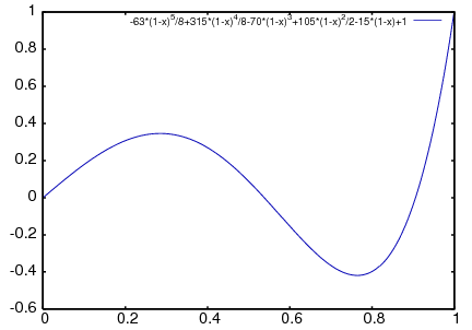
The entire expression legendre_p (5, x) is quoted; this is
different than just quoting the function name using 'legendre_p (5, x).
85.1.5 Miscellaneous Functions
The orthopoly package defines the
Pochhammer symbol and a unit step function. orthopoly uses
the Kronecker delta function and the unit step function in
gradef statements.
To convert Pochhammer symbols into quotients of gamma functions,
use makegamma.
(%i1) makegamma (pochhammer (x, n));
gamma(x + n)
(%o1) ------------
gamma(x)
(%i2) makegamma (pochhammer (1/2, 1/2));
1
(%o2) ---------
sqrt(%pi)
Derivatives of the Pochhammer symbol are given in terms of the psi
function.
(%i1) diff (pochhammer (x, n), x);
(%o1) (x) (psi (x + n) - psi (x))
n 0 0
(%i2) diff (pochhammer (x, n), n);
(%o2) (x) psi (x + n)
n 0
You need to be careful with the expression in (%o1); the difference of the
psi functions has polynomials when x = -1, -2, .., -n. These polynomials
cancel with factors in pochhammer (x, n) making the derivative a degree
n - 1 polynomial when n is a positive integer.
The Pochhammer symbol is defined for negative orders through its representation as a quotient of gamma functions. Consider
(%i1) q : makegamma (pochhammer (x, n));
gamma(x + n)
(%o1) ------------
gamma(x)
(%i2) sublis ([x=11/3, n= -6], q);
729
(%o2) - ----
2240
Alternatively, we can get this result directly.
(%i1) pochhammer (11/3, -6);
729
(%o1) - ----
2240
The unit step function is left-continuous; thus
(%i1) [unit_step (-1/10), unit_step (0), unit_step (1/10)]; (%o1) [0, 0, 1]
If you need a unit step function that is neither left or right continuous
at zero, define your own using signum; for example,
(%i1) xunit_step (x) := (1 + signum (x))/2$
(%i2) [xunit_step (-1/10), xunit_step (0), xunit_step (1/10)];
1
(%o2) [0, -, 1]
2
Do not redefine unit_step itself; some code in orthopoly
requires that the unit step function be left-continuous.
85.1.6 Algorithms
Generally, orthopoly does symbolic evaluation by using a hypergeometic
representation of the orthogonal polynomials. The hypergeometic
functions are evaluated using the (undocumented) functions hypergeo11
and hypergeo21. The exceptions are the half-integer Bessel functions
and the associated Legendre function of the second kind. The half-integer Bessel functions are
evaluated using an explicit representation, and the associated Legendre
function of the second kind is evaluated using recursion.
For floating point evaluation, we again convert most functions into a hypergeometic form; we evaluate the hypergeometic functions using forward recursion. Again, the exceptions are the half-integer Bessel functions and the associated Legendre function of the second kind. Numerically, the half-integer Bessel functions are evaluated using the SLATEC code.
Previous: Introduction to orthogonal polynomials, Up: Package orthopoly [Contents][Index]
85.2 Functions and Variables for orthogonal polynomials
- Function: assoc_legendre_p (n, m, x) 
The associated Legendre function of the first kind of degree n and order m, \(P_{n}^{m}(z),\) is a solution of the differential equation:
$$ (1-z^2){d^2 w\over dz^2} - 2z{dw\over dz} + \left[n(n+1)-{m^2\over 1-z^2}\right] w = 0 $$This is related to the Legendre polynomial, \(P_n(x)\) via
$$ P_n^m(x) = (-1)^m\left(1-x^2\right)^{m/2} {d^m\over dx^m} P_n(x) $$Reference: A&S eqn 22.5.37, A&S eqn 8.6.6, and A&S eqn 8.2.5.
Some examples:
(%i1) assoc_legendre_p(2,0,x); 2 3 (1 - x) (%o1) (- 3 (1 - x)) + ---------- + 1 2 (%i2) factor(%); 2 3 x - 1 (%o2) -------- 2 (%i3) factor(assoc_legendre_p(2,1,x)); 2 (%o3) - 3 x sqrt(1 - x ) (%i4) (-1)^1*(1-x^2)^(1/2)*diff(legendre_p(2,x),x); 2 (%o4) - (3 - 3 (1 - x)) sqrt(1 - x ) (%i5) factor(%); 2 (%o5) - 3 x sqrt(1 - x )Categories: Package orthopoly ·
- Function: assoc_legendre_q (n, m, x) 
The associated Legendre function of the second kind of degree n and order m, \(Q_{n}^{m}(z),\) is a solution of the differential equation:
$$ (1-z^2){d^2 w\over dz^2} - 2z{dw\over dz} + \left[n(n+1)-{m^2\over 1-z^2}\right] w = 0 $$Reference: Abramowitz and Stegun, equation 8.5.3 and 8.1.8.
Some examples:
(%i1) assoc_legendre_q(0,0,x); x + 1 log(- -----) x - 1 (%o1) ------------ 2 (%i2) assoc_legendre_q(1,0,x); x + 1 log(- -----) x - 2 x - 1 (%o2)/R/ ------------------ 2 (%i3) assoc_legendre_q(1,1,x); (%o3)/R/ x + 1 2 2 2 x + 1 2 log(- -----) sqrt(1 - x ) x - 2 sqrt(1 - x ) x - log(- -----) sqrt(1 - x ) x - 1 x - 1 - --------------------------------------------------------------------------- 2 2 x - 2Categories: Package orthopoly ·
- Function: chebyshev_t (n, x) 
The Chebyshev polynomial of the first kind of degree n, \(T_n(x).\)
Reference: A&S eqn 22.5.47.
The polynomials \(T_n(x)\) can be written in terms of a hypergeometric function:
$$ T_n(x) = {_{2}}F_{1}\left(-n, n; {1\over 2}; {1-x\over 2}\right) $$The polynomials can also be defined in terms of the sum
$$ T_n(x) = {n\over 2} \sum_{r=0}^{\lfloor {n/2}\rfloor} {(-1)^r\over n-r} {n-r\choose k}(2x)^{n-2r} $$or the Rodrigues formula
$$ T_n(x) = {1\over \kappa_n w(x)} {d^n\over dx^n}\left(w(x)(1-x^2)^n\right) $$where
$$ \eqalign{ w(x) &= 1/\sqrt{1-x^2} \cr \kappa_n &= (-2)^n\left(1\over 2\right)_n } $$Some examples:
(%i1) chebyshev_t(2,x); 2 (%o1) (- 4 (1 - x)) + 2 (1 - x) + 1 (%i2) factor(%); 2 (%o2) 2 x - 1 (%i3) factor(chebyshev_t(3,x)); 2 (%o3) x (4 x - 3) (%i4) factor(hgfred([-3,3],[1/2],(1-x)/2)); 2 (%o4) x (4 x - 3)Categories: Package orthopoly ·
- Function: chebyshev_u (n, x) 
The Chebyshev polynomial of the second kind of degree n, \(U_n(x).\)
Reference: A&S eqn 22.5.48.
The polynomials \(U_n(x)\) can be written in terms of a hypergeometric function:
$$ U_n(x) = (n+1)\; {_{2}F_{1}}\left(-n, n+2; {3\over 2}; {1-x\over 2}\right) $$The polynomials can also be defined in terms of the sum
$$ U_n(x) = \sum_{r=0}^{\lfloor n/2 \rfloor} (-1)^r {n-r \choose r} (2x)^{n-2r} $$or the Rodrigues formula
$$ U_n(x) = {1\over \kappa_n w(x)} {d^n\over dx^n}\left(w(x)(1-x^2)^n\right) $$where
$$ \eqalign{ w(x) &= \sqrt{1-x^2} \cr \kappa_n &= {(-2)^n\left({3\over 2}\right)_n \over n+1} } $$.
(%i1) chebyshev_u(2,x); 2 8 (1 - x) 4 (1 - x) (%o1) 3 ((- ---------) + ---------- + 1) 3 3 (%i2) expand(%); 2 (%o2) 4 x - 1 (%i3) expand(chebyshev_u(3,x)); 3 (%o3) 8 x - 4 x (%i4) expand(4*hgfred([-3,5],[3/2],(1-x)/2)); 3 (%o4) 8 x - 4 xCategories: Package orthopoly ·
- Function: gen_laguerre (n, a, x) 
The generalized Laguerre polynomial of degree n, \(L_n^{(\alpha)}(x).\)
These can be defined by
$$ L_n^{(\alpha)}(x) = {n+\alpha \choose n}\; {_1F_1}(-n; \alpha+1; x) $$The polynomials can also be defined by the sum
$$ L_n^{(\alpha)}(x) = \sum_{k=0}^n {(\alpha + k + 1)_{n-k} \over (n-k)! k!} (-x)^k $$or the Rodrigues formula
$$ L_n^{(\alpha)}(x) = {1\over \kappa_n w(x)} {d^n\over dx^n}\left(w(x)x^n\right) $$where
$$ \eqalign{ w(x) &= e^{-x}x^{\alpha} \cr \kappa_n &= n! } $$Reference: A&S eqn 22.5.54.
Some examples:
(%i1) gen_laguerre(1,k,x); x (%o1) (k + 1) (1 - -----) k + 1 (%i2) gen_laguerre(2,k,x); 2 x 2 x (k + 1) (k + 2) (--------------- - ----- + 1) (k + 1) (k + 2) k + 1 (%o2) --------------------------------------------- 2 (%i3) binomial(2+k,2)*hgfred([-2],[1+k],x); 2 x 2 x (k + 1) (k + 2) (--------------- - ----- + 1) (k + 1) (k + 2) k + 1 (%o3) --------------------------------------------- 2Categories: Package orthopoly ·
- Function: hermite (n, x) 
The Hermite polynomial of degree n, \(H_n(x).\)
These polynomials may be defined by a hypergeometric function
$$ H_n(x) = (2x)^n\; {_2F_0}\left(-{1\over 2} n, -{1\over 2}n+{1\over 2};;-{1\over x^2}\right) $$or by the series
$$ H_n(x) = n! \sum_{k=0}^{\lfloor n/2 \rfloor} {(-1)^k(2x)^{n-2k} \over k! (n-2k)!} $$or the Rodrigues formula
$$ H_n(x) = {1\over \kappa_n w(x)} {d^n\over dx^n}\left(w(x)\right) $$where
$$ \eqalign{ w(x) &= e^{-{x^2/2}} \cr \kappa_n &= (-1)^n } $$Reference: A&S eqn 22.5.55.
Some examples:
(%i1) hermite(3,x); 2 2 x (%o1) - 12 x (1 - ----) 3 (%i2) expand(%); 3 (%o2) 8 x - 12 x (%i3) expand(hermite(4,x)); 4 2 (%o3) 16 x - 48 x + 12 (%i4) expand((2*x)^4*hgfred([-2,-2+1/2],[],-1/x^2)); 4 2 (%o4) 16 x - 48 x + 12 (%i5) expand(4!*sum((-1)^k*(2*x)^(4-2*k)/(k!*(4-2*k)!),k,0,floor(4/2))); 4 2 (%o5) 16 x - 48 x + 12Categories: Package orthopoly ·
- Function: intervalp (e) 
Return
trueif the input is an interval and return false if it isn’t.Categories: Package orthopoly · Predicate functions ·
- Function: jacobi_p (n, a, b, x) 
The Jacobi polynomial, \(P_n^{(a,b)}(x).\)
The Jacobi polynomials are actually defined for all a and b; however, the Jacobi polynomial weight (1 - x)^a (1 + x)^b isn’t integrable for \(a \le -1\) or \(b \le -1.\)
Reference: A&S eqn 22.5.42.
The polynomial may be defined in terms of hypergeometric functions:
$$ P_n^{(a,b)}(x) = {n+a\choose n} {_1F_2}\left(-n, n + a + b + 1; a+1; {1-x\over 2}\right) $$or the Rodrigues formula
$$ P_n^{(a, b)}(x) = {1\over \kappa_n w(x)} {d^n\over dx^n}\left(w(x)\left(1-x^2\right)^n\right) $$where
$$ \eqalign{ w(x) &= (1-x)^a(1-x)^b \cr \kappa_n &= (-2)^n n! } $$Some examples:
(%i1) jacobi_p(0,a,b,x); (%o1) 1 (%i2) jacobi_p(1,a,b,x); (b + a + 2) (1 - x) (%o2) (a + 1) (1 - -------------------) 2 (a + 1)Categories: Package orthopoly ·
- Function: laguerre (n, x) 
The Laguerre polynomial, \(L_n(x)\) of degree n.
Reference: A&S eqn 22.5.16 and A&S eqn 22.5.54.
These are related to the generalized Laguerre polynomial by
$$ L_n(x) = L_n^{(0)}(x) $$The polynomials are given by the sum
$$ L_n(x) = \sum_{k=0}^{n} {(-1)^k\over k!}{n \choose k} x^k $$Some examples:
(%i1) laguerre(1,x); (%o1) 1 - x (%i2) laguerre(2,x); 2 x (%o2) -- - 2 x + 1 2 (%i3) gen_laguerre(2,0,x); 2 x (%o3) -- - 2 x + 1 2 (%i4) sum((-1)^k/k!*binomial(2,k)*x^k,k,0,2); 2 x (%o4) -- - 2 x + 1 2Categories: Package orthopoly ·
- Function: legendre_p (n, x) 
The Legendre polynomial of the first kind, \(P_n(x),\) of degree n.
Reference: A&S eqn 22.5.50 and A&S eqn 22.5.51.
The Legendre polynomial is related to the Jacobi polynomials by
$$ P_n(x) = P_n^{(0,0)}(x) $$or the Rodrigues formula
$$ P_n(x) = {1\over \kappa_n w(x)} {d^n\over dx^n}\left(w(x)\left(1-x^2\right)^n\right) $$where
$$ \eqalign{ w(x) &= 1 \cr \kappa_n &= (-2)^n n! } $$Some examples:
(%i1) legendre_p(1,x); (%o1) x (%i2) legendre_p(2,x); 2 3 (1 - x) (%o2) (- 3 (1 - x)) + ---------- + 1 2 (%i3) expand(%); 2 3 x 1 (%o3) ---- - - 2 2 (%i4) expand(legendre_p(3,x)); 3 5 x 3 x (%o4) ---- - --- 2 2 (%i5) expand(jacobi_p(3,0,0,x)); 3 5 x 3 x (%o5) ---- - --- 2 2Categories: Package orthopoly ·
- Function: legendre_q (n, x) 
The Legendre function of the second kind, \(Q_n(x)\) of degree n.
Reference: Abramowitz and Stegun, equations 8.5.3 and 8.1.8.
These are related to \(Q_n^m(x)\) by
$$ Q_n(x) = Q_n^0(x) $$Some examples:
(%i1) legendre_q(0,x); x + 1 log(- -----) x - 1 (%o1) ------------ 2 (%i2) legendre_q(1,x); x + 1 log(- -----) x - 2 x - 1 (%o2)/R/ ------------------ 2 (%i3) assoc_legendre_q(1,0,x); x + 1 log(- -----) x - 2 x - 1 (%o3)/R/ ------------------ 2Categories: Package orthopoly ·
- Function: orthopoly_recur (f, args) 
Returns a recursion relation for the orthogonal function family f with arguments args. The recursion is with respect to the polynomial degree.
(%i1) orthopoly_recur (legendre_p, [n, x]); (2 n + 1) P (x) x - n P (x) n n - 1 (%o1) P (x) = ------------------------------- n + 1 n + 1The second argument to
orthopoly_recurmust be a list with the correct number of arguments for the function f; if it isn’t, Maxima signals an error.(%i1) orthopoly_recur (jacobi_p, [n, x]); Function jacobi_p needs 4 arguments, instead it received 2 -- an error. Quitting. To debug this try debugmode(true);
Additionally, when f isn’t the name of one of the families of orthogonal polynomials, an error is signalled.
(%i1) orthopoly_recur (foo, [n, x]); A recursion relation for foo isn't known to Maxima -- an error. Quitting. To debug this try debugmode(true);
Categories: Package orthopoly ·
- Variable: orthopoly_returns_intervals 
Default value:
trueWhen
orthopoly_returns_intervalsistrue, floating point results are returned in the forminterval (c, r), where c is the center of an interval and r is its radius. The center can be a complex number; in that case, the interval is a disk in the complex plane.Categories: Package orthopoly ·
- Function: orthopoly_weight (f, args) 
-
Returns a three element list; the first element is the formula of the weight for the orthogonal polynomial family f with arguments given by the list args; the second and third elements give the lower and upper endpoints of the interval of orthogonality. For example,
(%i1) w : orthopoly_weight (hermite, [n, x]); 2 - x (%o1) [%e , - inf, inf] (%i2) integrate(w[1]*hermite(3, x)*hermite(2, x), x, w[2], w[3]); (%o2) 0The main variable of f must be a symbol; if it isn’t, Maxima signals an error.
Categories: Package orthopoly ·
- Function: pochhammer (x, n) 
The Pochhammer symbol, \((x)_n.\) (See A&S eqn 6.1.22 and DLMF 5.2.iii).
For nonnegative integers n with
n <= pochhammer_max_index, the expression \((x)_n\) evaluates to the product \(x(x+1)(x+2)\cdots(x+n-1)\) when \(n > 0\) and to 1 when n = 0. For negative n, \((x)_n\) is defined as \((-1)^n/(1-x)_{-n}.\) Thus(%i1) pochhammer (x, 3); (%o1) x (x + 1) (x + 2) (%i2) pochhammer (x, -3); 1 (%o2) - ----------------------- (1 - x) (2 - x) (3 - x)To convert a Pochhammer symbol into a quotient of gamma functions, (see A&S eqn 6.1.22) use
makegamma; for example(%i1) makegamma (pochhammer (x, n)); gamma(x + n) (%o1) ------------ gamma(x)When n exceeds
pochhammer_max_indexor when n is symbolic,pochhammerreturns a noun form.(%i1) pochhammer (x, n); (%o1) (x) nCategories: Package orthopoly · Gamma and factorial functions ·
- Variable: pochhammer_max_index 
Default value: 100
pochhammer (n, x)expands to a product if and only ifn <= pochhammer_max_index.Examples:
(%i1) pochhammer (x, 3), pochhammer_max_index : 3; (%o1) x (x + 1) (x + 2) (%i2) pochhammer (x, 4), pochhammer_max_index : 3; (%o2) (x) 4Reference: A&S eqn 6.1.16.
Categories: Package orthopoly · Gamma and factorial functions ·
- Function: spherical_bessel_j (n, x) 
The spherical Bessel function of the first kind, \(j_n(x).\)
Reference: A&S eqn 10.1.8 and A&S eqn 10.1.15.
It is related to the Bessel function by
$$ j_n(x) = \sqrt{\pi\over 2x} J_{n+1/2}(x) $$Some examples:
(%i1) spherical_bessel_j(1,x); sin(x) ------ - cos(x) x (%o1) --------------- x (%i2) spherical_bessel_j(2,x); 3 3 cos(x) (- (1 - --) sin(x)) - -------- 2 x x (%o2) ------------------------------ x (%i3) expand(%); sin(x) 3 sin(x) 3 cos(x) (%o3) (- ------) + -------- - -------- x 3 2 x x (%i4) expand(sqrt(%pi/(2*x))*bessel_j(2+1/2,x)),besselexpand:true; sin(x) 3 sin(x) 3 cos(x) (%o4) (- ------) + -------- - -------- x 3 2 x xCategories: Package orthopoly · Bessel functions ·
- Function: spherical_bessel_y (n, x) 
The spherical Bessel function of the second kind, \(y_n(x).\)
Reference: A&S eqn 10.1.9 and A&S eqn 10.1.15.
It is related to the Bessel function by
$$ y_n(x) = \sqrt{\pi\over 2x} Y_{n+1/2}(x) $$(%i1) spherical_bessel_y(1,x); cos(x) (- sin(x)) - ------ x (%o1) ------------------- x (%i2) spherical_bessel_y(2,x); 3 sin(x) 3 -------- - (1 - --) cos(x) x 2 x (%o2) - -------------------------- x (%i3) expand(%); 3 sin(x) cos(x) 3 cos(x) (%o3) (- --------) + ------ - -------- 2 x 3 x x (%i4) expand(sqrt(%pi/(2*x))*bessel_y(2+1/2,x)),besselexpand:true; 3 sin(x) cos(x) 3 cos(x) (%o4) (- --------) + ------ - -------- 2 x 3 x xCategories: Package orthopoly · Bessel functions ·
- Function: spherical_hankel1 (n, x) 
The spherical Hankel function of the first kind, \(h_n^{(1)}(x).\)
Reference: A&S eqn 10.1.36.
This is defined by
$$ h_n^{(1)}(x) = j_n(x) + iy_n(x) $$Categories: Package orthopoly · Bessel functions ·
- Function: spherical_hankel2 (n, x) 
The spherical Hankel function of the second kind, \(h_n^{(2)}(x).\)
Reference: A&S eqn 10.1.17.
This is defined by
$$ h_n^{(2)}(x) = j_n(x) + iy_n(x) $$Categories: Package orthopoly · Bessel functions ·
- Function: spherical_harmonic (n, m, theta, phi) 
The spherical harmonic function, \(Y_n^m(\theta, \phi).\)
Spherical harmonics satisfy the angular part of Laplace’s equation in spherical coordinates.
For integers n and m such that \(n \geq |m|\) and for \(\theta \in [0, \pi].\) Maxima’s spherical harmonic function can be defined by
$$ Y_n^m(\theta, \phi) = (-1)^m \sqrt{{2n+1\over 4\pi} {(n-m)!\over (n+m)!}} P_n^m(\cos\theta) e^{im\phi} $$Further, when \(n < |m|,\) the spherical harmonic function vanishes.
The factor (-1)^m, frequently used in Quantum mechanics, is called the Condon-Shortely phase. Some references, including NIST Digital Library of Mathematical Functions omit this factor; see http://dlmf.nist.gov/14.30.E1.
Reference: Merzbacher 9.64.
Some examples:
(%i1) spherical_harmonic(1,0,theta,phi); sqrt(3) cos(theta) (%o1) ------------------ 2 sqrt(%pi) (%i2) spherical_harmonic(1,1,theta,phi); %i phi sqrt(3) %e sin(theta) (%o2) --------------------------- 3/2 2 sqrt(%pi) (%i3) spherical_harmonic(1,-1,theta,phi); - %i phi sqrt(3) %e sin(theta) (%o3) - ----------------------------- 3/2 2 sqrt(%pi) (%i4) spherical_harmonic(2,0,theta,phi); 2 3 (1 - cos(theta)) sqrt(5) ((- 3 (1 - cos(theta))) + ------------------- + 1) 2 (%o4) ---------------------------------------------------------- 2 sqrt(%pi) (%i5) factor(%); 2 sqrt(5) (3 cos (theta) - 1) (%o5) --------------------------- 4 sqrt(%pi)Categories: Package orthopoly ·
- Function: unit_step (x) 
The left-continuous unit step function; thus
unit_step (x)vanishes forx <= 0and equals 1 forx > 0.If you want a unit step function that takes on the value 1/2 at zero, use
hstep.Categories: Package orthopoly · Mathematical functions ·
- Function: ultraspherical (n, a, x) 
The ultraspherical polynomial, \(C_n^{(a)}(x)\) (also known as the Gegenbauer polynomial).
Reference: A&S eqn 22.5.46.
These polynomials can be given in terms of Jacobi polynomials:
$$ C_n^{(\alpha)}(x) = {\Gamma\left(\alpha + {1\over 2}\right) \over \Gamma(2\alpha)} {\Gamma(n+2\alpha) \over \Gamma\left(n+\alpha + {1\over 2}\right)} P_n^{(\alpha-1/2, \alpha-1/2)}(x) $$or the series
$$ C_n^{(\alpha)}(x) = \sum_{k=0}^{\lfloor n/2 \rfloor} {(-1)^k (\alpha)_{n-k} \over k! (n-2k)!}(2x)^{n-2k} $$or the Rodrigues formula
$$ C_n^{(\alpha)}(x) = {1\over \kappa_n w(x)} {d^n\over dx^n}\left(w(x)\left(1-x^2\right)^n\right) $$where
$$ \eqalign{ w(x) &= \left(1-x^2\right)^{\alpha-{1\over 2}} \cr \kappa_n &= {(-2)^n\left(\alpha + {1\over 2}\right)_n n!\over (2\alpha)_n} \cr } $$Some examples:
(%i1) ultraspherical(1,a,x); (2 a + 1) (1 - x) (%o1) 2 a (1 - -----------------) 1 2 (a + -) 2 (%i2) factor(%); (%o2) 2 a x (%i3) factor(ultraspherical(2,a,x)); 2 2 (%o3) a (2 a x + 2 x - 1)Categories: Package orthopoly ·
Next: Package pytranslate, Previous: Package orthopoly [Contents][Index]
86 Package pslq
Next: Functions and Variables for pslq, Previous: Package pslq, Up: Package pslq [Contents][Index]
86.1 Introduction to pslq
Package pslq contains two functions.
(1) guess_exact_value tries to find
an exact equivalent for an inexact number (float or bigfloat).
(2) pslq_integer_relation tries to find
integer coefficients such that a linear combination of inexact numbers
is approximately zero.
Previous: Introduction to pslq, Up: Package pslq [Contents][Index]
86.2 Functions and Variables for pslq
- Function: guess_exact_value (x) 
-
When x is a floating point number or bigfloat,
guess_exact_valuetries to find an exact expression (in terms of radicals, logarithms, exponentials, and the constant%pi) which is nearly equal to the given number. Ifguess_exact_valuecannot find such an expression, x is returned unchanged.When x is rational number or other mapatom (other than a float or bigfloat), x is returned unchanged.
Otherwise, x is a nonatomic expression, and
guess_exact_valueis applied to each of the arguments of x.Example:
(%i1) load ("pslq.mac"); (%o1) pslq.mac (%i2) root: float (sin (%pi/12)); (%o2) 0.2588190451025207 (%i3) guess_exact_value (root); sqrt(2 - sqrt(3)) (%o3) ----------------- 2 (%i4) L: makelist (root^i, i, 0, 4); (%o4) [1.0, 0.2588190451025207, 0.06698729810778066, 0.01733758853025369, 0.004487298107780675] (%i5) m: pslq_integer_relation(%); (%o5) [- 1, 0, 16, 0, - 16] (%i6) makelist (x^i, i, 0, 4) . m; 4 2 (%o6) (- 16 x ) + 16 x - 1 (%i7) solve(%); sqrt(sqrt(3) + 2) sqrt(sqrt(3) + 2) (%o7) [x = - -----------------, x = -----------------, 2 2 sqrt(2 - sqrt(3)) sqrt(2 - sqrt(3)) x = - -----------------, x = -----------------] 2 2
- Function: pslq_integer_relation (L) 
-
Implements the PSLQ algorithm [1] to find integer relations between bigfloat numbers.
For a given list L of floating point numbers,
pslq_integer_relationreturns a list of integers m such thatm . L = 0(with absolute residual error less thanpslq_threshold).[1] D.H.Bailey: Integer Relation Detection and Lattice Reduction.
Example:
(%i1) load ("pslq.mac"); (%o1) pslq.mac (%i2) root: float (sin (%pi/12)); (%o2) 0.2588190451025207 (%i3) L: makelist (root^i, i, 0, 4); (%o3) [1.0, 0.2588190451025207, 0.06698729810778066, 0.01733758853025369, 0.004487298107780675] (%i4) m: pslq_integer_relation(%); (%o4) [- 1, 0, 16, 0, - 16] (%i5) m . L; (%o5) - 2.359223927328458E-16 (%i6) float (10^(2 - fpprec)); (%o6) 1.0E-14 (%i7) is (abs (m . L) < 10^(2 - fpprec)); (%o7) true
- Variable: pslq_precision 
Default value:
10^(fpprec - 2)Maximum magnitude of some intermediate results in
pslq_integer_relation. The search fails if one of the intermediate results has elements larger thanpslq_precision.
- Variable: pslq_threshold 
Default value:
10^(2 - fpprec)Threshold for absolute residual error of integer relation found by
pslq_integer_relation.
- Variable: pslq_depth 
Default value:
20 * nNumber of iterations of the PSLQ algorithm.
The default value is 20 times n, where n is the length of the list of numbers supplied to
pslq_integer_relation.
- Variable: pslq_status 
-
Indicates success or failure for an integer relation search by
pslq_integer_relation.When
pslq_statusis 1, it indicates an integer relation was found, and the absolute residual error is less thanpslq_threshold.When
pslq_statusis 2, it indicates an integer relation was not found because some intermediate results are larger thanpslq_precision.When
pslq_statusis 3, it indicates an integer relation was not found because the number of iterationspslq_depthwas reached.
Next: Package quantum_computing, Previous: Package pslq [Contents][Index]
87 Package pytranslate
Next: Functions in pytranslate, Up: Package pytranslate [Contents][Index]
87.1 Introduction to pytranslate
pytranslate package provides Maxima to Python translation functionality. The package is experimental, and the specifications of the functions in this package might change. It was written as a Google Summer of Code project by Lakshya A Agrawal (Undergraduate Student, IIIT-Delhi) in 2019. A detailed project report is available as a GitHub Gist.
The package needs to be loaded in a Maxima instance for use, by executing load("pytranslate");
The statements are converted to python3 syntax. The file pytranslate.py must be imported for all translations to run, as shown in example.
Example:
(%i1) load ("pytranslate")$
/* Define an example function to calculate factorial */
(%i2) pytranslate(my_factorial(x) := if (x = 1 or x = 0) then 1
else x * my_factorial(x - 1));
(%o2)
def my_factorial(x, v = v):
v = Stack({}, v)
v.ins({"x" : x})
return((1 if ((v["x"] == 1) or (v["x"] == 0)) \
else (v["x"] * my_factorial((v["x"] + (-1))))))
m["my_factorial"] = my_factorial
(%i3) my_factorial(5); (%o3) 120
>>> from pytranslate import *
>>> def my_factorial(x, v = v):
... v = Stack({}, v)
... v.ins({"x" : x})
... return((1 if ((v["x"] == 1) or (v["x"] == 0)) \
... else (v["x"] * my_factorial((v["x"] + (-1))))))
...
>>> my_factorial(5)
120
The Maxima to Python Translator works in two stages:
1. Conversion of the internal Maxima representation to a defined Intermediate Representation, henceforth referred as IR(mapping is present in share/pytranslate/maxima-to-ir.html)
2. The conversion of IR to Python.
Supported Maxima forms:
1. Numbers(including complex numbers)
2. Assignment operators
3. Arithmetic operators(+, -, *, ^, /, !)
4. Logical operators(and, or, not)
5. Relational operators(>, <, >=, <=, !=, ==)
6. Lists
7. Arrays
8. block
9. Function and function calls
10. if-else converted to Python conditionals
11. for loops
12. lambda form
87.1.1 Tests for pytranslate
The tests for pytranslate are present at share/pytranslate/rtest_pytranslate.mac and can be run by executing batch(rtest_pytranslate, test);
Next: Extending pytranslate, Previous: Introduction to pytranslate, Up: Package pytranslate [Contents][Index]
87.2 Functions in pytranslate
- Function: pytranslate (expr, [print-ir]) 
Translates the expression expr to equivalent python3 statements. Output is printed in the stdout.
Example:
(%i1) load ("pytranslate")$(%i2) pytranslate('(for i:8 step -1 unless i<3 do (print(i)))); (%o2) v["i"] = 8 while not((v["i"] < 3)): m["print"](v["i"]) v["i"] = (v["i"] + -1) del v["i"]expr is evaluated, and the return value is used for translation. Hence, for statements like assignment, it might be useful to quote the statement:
(%i1) load ("pytranslate")$(%i2) pytranslate(x:20); (%o2) 20
(%i3) pytranslate('(x:20)); (%o3) v["x"] = 20Passing the optional parameter (print-ir) to
pytranslateas t, will print the internal IR representation ofexprand return the translated python3 code.(%i1) load("pytranslate"); (%o1) pytranslate(%i2) pytranslate('(plot3d(lambda([x, y], x^2+y^(-1)), [x, 1, 10], [y, 1, 10])), t); (body (funcall (element-array "m" (string "plot3d")) (lambda ((symbol "x") (symbol "y") (op-no-bracket = (symbol "v") (funcall (symbol "stack") (dictionary) (symbol "v")))) (op + (funcall (element-array (symbol "m") (string "pow")) (symbol "x") (num 2 0)) (funcall (element-array (symbol "m") (string "pow")) (symbol "y") (unary-op - (num 1 0))))) (struct-list (string "x") (num 1 0) (num 10 0)) (struct-list (string "y") (num 1 0) (num 10 0)))) (%o2) m["plot3d"](lambda x, y, v = Stack({}, v): (m["pow"](x, 2) + m["\ pow"](y, (-1))), ["x", 1, 10], ["y", 1, 10])
- Function: show_form (expr) 
Displays the internal maxima form of
expr(%i4) show_form(a^b); ((mexpt) $a $b) (%o4) a^b
Previous: Functions in pytranslate, Up: Package pytranslate [Contents][Index]
87.3 Extending pytranslate
Working of pytranslate:
- The entry point for pytranslate is the function
$pytranslatedefined in share/pytranslate/pytranslate.lisp. -
$pytranslatecalls the functionmaxima-to-irwith the Maxima expression as an argument(henceforth referred asexpr). -
maxima-to-irdetermines ifexpris atomic or non-atomic(lisp cons form). If atomic,atom-to-iris called withexprwhich returns the IR for the atomic expression.
To define/modify translation for atomic expressions, make changes to the definition ofatom-to-irin accordance with the IR. - If
expris non-atomic, the functioncons-to-iris called withexpras an argument.
-
cons-to-irlooks for(caar expr)which specifies the type ofexpr, in hash-table *maxima-direct-ir-map* and if the type is found, then appends the retrieved IR with the result of lisp call(mapcar #'maxima-to-ir (cdr expr)), which applies maxima-to-ir function to all the elements present in the list. Effectively, recursively generate IR for all the elements present inexprand append them to the IR map for the type.
Example:(%i9) show_form(a+b); ((MPLUS) $B $A)
(%i10) pytranslate(a+b, t); (body (op + (element-array (symbol "v") (string "b")) \ (element-array (symbol "v") (string "a")))) (%o10) (v["b"] + v["a"])
Here, operator + with internal maxima representation,
(mplus)is present in *maxima-direct-ir-map* and mapped to(op +)to which the result of generating IR for all other elements of the list (a b), i.e.(ELEMENT-ARRAY (SYMBOL "v") (STRING "b")) (ELEMENT-ARRAY (SYMBOL "v") (STRING "a"))is appended.
- If
(caar expr)is not found in *maxima-direct-ir-map*, thencons-to-irlooks for the type in *maxima-special-ir-map* which returns the function to handle the translation of the type ofexpr.cons-to-irthen calls the returned function with argumentexpras an argument.
Example:(%i11) show_form(g(x) := x^2); ((mdefine simp) (($g) $x) ((mexpt) $x 2))
(%i12) pytranslate(g(x):=x^2, t); (body (body (func-def (symbol "g") ((symbol "x") (op-no-bracket = (symbol "v") (symbol "v"))) (body-indented (op-no-bracket = (symbol "v") (funcall (symbol "stack") \ (dictionary) (symbol "v"))) (obj-funcall (symbol "v") (symbol "ins") (dictionary \ ((string "x") (symbol "x")))) (funcall (symbol "return") (funcall (element-array (symbol "f") (string "pow")) (element-array (symbol "v") (string "x")) (num 2 0))))) (op-no-bracket = (element-array (symbol "f") (string "g")) \ (symbol "g")))) (%o12) def g(x, v = v): v = Stack({}, v) v.ins({"x" : x}) return(f["pow"](v["x"], 2)) f["g"] = gHere,
mdefine, which is the type ofexpris present in *maxima-special-ir-map* which returnsfunc-def-to-iras handler function, which is then called withexprto generate the IR.
To define/modify translation for a type, add an entry to *maxima-direct-ir-map* if only a part of the IR needs to be generated and the rest can be appended, otherwise, for complete handling ofexpr, add an entry to *maxima-special-ir-map* and define a function with the name defined in *maxima-special-ir-map* which returns the IR for the form. The function naming convention for ir generators is (type)-to-ir, where type is the(caar expr)for expression(mdefine -> func-def-to-ir). The function must return a valid IR for the specific type.
-
- After the generation of IR, the function
ir-to-pythonis called with the generatediras an argument, which performs the codegen in a recursive manner.-
ir-to-pythonlooks for lisp(car ir)in the hash-table *ir-python-direct-templates*, which maps IR type to function handlers and calls the function returned withiras an argument.
-
- To extend the IR of pytranslate, define a function with the naming convention (type)-to-python and add the name to *ir-python-direct-templates*.
Next: Package ratpow, Previous: Package pytranslate [Contents][Index]
88 Package quantum_computing
Next: Functions and Variables for Quantum_Computing, Previous: Package quantum_computing, Up: Package quantum_computing [Contents][Index]
88.1 Package quantum_computing
The quantum_computing package provides several functions to
simulate quantum computing circuits. The state of a system of n
qubits is represented by a list of 2^n complex numbers and an
operator acting on m qubits is represented by a 2^m by
2^m matrix. A hash array qmatrix is defined with 6 common
one-qubit matrices: the identity, the Pauli matrices, the Hadamard
matrix and the phase matrix.
The major disadvantage compared to a real quantum computer is very slow
computing times even with a few qubits. An advantage is that, unlike a
quantum computer, in this simulator a quantum state can be cloned using
copylist.
This is an additional package that must be loaded with
load("quantum_computing") in order to use it.
Previous: Package quantum_computing, Up: Package quantum_computing [Contents][Index]
88.2 Functions and Variables for Quantum_Computing
- Function: binlist
binlist (k)
binlist (k, n) ¶ -
binlist(k), where k must be a natural number, returns a list of binary digits 0 or 1 corresponding to the digits of k in binary representation.binlist(k, n) does the same but returns a list of length n, with leading zeros as necessary. Notice that for the result to represent a possible state of m qubits, n should be equal to 2^m and k should be between 0 and 2^m-1.Categories: Package quantum_computing ·
- Function: binlist2dec (lst) 
-
Given a list lst with n binary digits, it returns the decimal number it represents.
Categories: Package quantum_computing ·
- Function: CNOT (q, i, j) 
-
Changes the value of the j’th qubit, in a state q of m qubits, when the value of the i’th qubit equals 1. It modifies the list q and returns its modified value.
Categories: Package quantum_computing ·
- Function: controlled (U, q, c, i) 
-
Applies a matrix U, acting on m qubits, on qubits i through i+m-1 of the state q of n qubits (n > m), when the value of the c’th qubit in q equals 1. i should be an integer between 1 and n+1-m and c should be an integer between 1 and n, excluding the qubits to be modified (i through i+m-1).
U can be one of the indices of the array of common matrices qmatrix (see
qmatrix). The state q is modified and shown in the output.Categories: Package quantum_computing ·
- Function: gate
gate (U, q)
gate (U, q, i)
gate (U, q, i1, …, im) ¶ -
U must be a matrix acting on states of m qubits; q a list corresponding to a state of n qubits (n >= m); i and the m numbers i1, …, im must be different integers between 1 and n.
gate(U, q) applies matrix U to each qubit of q, when m equals 1, or to the first m qubits of q when m is bigger than 1.gate(U, q, i) applies matrix U to the qubits i through i+m-1 of q.gate(U, q, i1, …, in) applies matrix U to the in the positions i1, …, im.U can be one of the indices of the array of common matrices qmatrix (see
qmatrix). The state q is modified and shown in the output.Categories: Package quantum_computing ·
- Function: gate_matrix
gate_matrix (U, n)
gate_matrix (U, n, i1, …, im) ¶ -
U must be a 2 by 2 matrix or one of the indices of the array of common matrices qmatrix (see
qmatrix).gate_matrix(U, n) returns the matrix corresponding to the action of U on each qubit in a state of n qubits.gate_matrix(U, n, i1, …, im) returns the matrix corresponding to the action of U on qubits i1, …, im of a state of n qubits, where i1, …, im are different integers between 1 and n.Categories: Package quantum_computing ·
- Function: linsert (e, lst, p) 
-
Inserts the expression or list e into the list lst at position p. The list can be empty and p must be an integer between 1 and the length of lst plus 1.
Categories: Package quantum_computing ·
- Function: lreplace (e, lst, p) 
-
If e is a list of length n, the elements in the positions p, p+1, …, p+n-1 of the list lst are replaced by e, or the first elements of e if the end of lst is reached. If e is an expression, the element in position p of list lst is replaced by that expression. p must be an integer between 1 and the length of lst.
Categories: Package quantum_computing ·
- Function: normalize (q) 
-
Returns the normalized version of a quantum state given as a list q.
Categories: Package quantum_computing ·
- Function: qdisplay (q) 
-
Represents the state q of a system of n qubits as a linear combination of the computational states with n binary digits. It returns an expression including strings and symbols.
Categories: Package quantum_computing ·
- System variable: qmatrix 
-
This variable is a predefined hash array of two by two matrices with the standard matrices: identity, Pauli matrices, Hadamard matrix and the phase matrix. The six possible indices are I, X, Y, Z, H, S. qmatrix[I] is the identity matrix, qmatrix[X] the Pauli x matrix, qmatrix[Y] the Pauli y matrix, qmatrix[Z] the Pauli z matrix, qmatrix[H] the Hadamard matrix and qmatrix[S] the phase matrix.
Categories: Package quantum_computing ·
- Function: qmeasure
qmeasure (q)
qmeasure (q, i1, …, im) ¶ -
Measures the value of one or more qubits in a system of n qubits with state q. The m positive integers i1, …, im are the positions of the qubits to be measured It requires 1 or more arguments. The first argument must be the state q. If the only argument given is q, all the n qubits will be measured.
It returns a list with the values of the qubits measured (either 0 or 1), in the same order they were requested or in ascending order if the only argument given was q. It modifies the list q, reflecting the collapse of the quantum state after the measurement.
Categories: Package quantum_computing ·
- Function: qubits
qubits (n)
qubits (i1, …, in) ¶ -
qubits(n) returns a list representing the ground state of a system of n qubits.qubits(i1, …, in) returns a list with representing the state of n qubits with values i1, …, in.Categories: Package quantum_computing ·
- Function: qswap (q, i, j) 
-
Interchanges the states of qubits i and j in the state q of a system of several qubits. It modifies the list q and returns its modified value.
Categories: Package quantum_computing ·
- Function: Rx (a) 
-
Returns the 2 by two matrix (acting on one qubit) corresponding to a rotation of with an angle of a radians around the x axis.
Categories: Package quantum_computing ·
- Function: Ry (a) 
-
Returns the 2 by two matrix (acting on one qubit) corresponding to a rotation of with an angle of a radians around the y axis.
Categories: Package quantum_computing ·
- Function: Rz (a) 
-
Returns the 2 by two matrix (acting on one qubit) corresponding to a rotation of with an angle of a radians around the z axis.
Categories: Package quantum_computing ·
- Function: tprod (o1, …, on) 
-
Returns the tensor product of the n matrices or lists o1, …, on.
Categories: Package quantum_computing ·
- Function: toffoli (q, (i, (j, (k) 
-
Changes the value of the k’th qubit, in the state q of n qubits, if the values of the i’th anf j’th qubits are equal to 1. It modifies the list q and returns its new value.
Categories: Package quantum_computing ·
Next: Package romberg, Previous: Package quantum_computing [Contents][Index]
89 Package ratpow
The package ratpow provides functions that return the coefficients
of the numerator of a CRE polynomial in a given variable.
For example,
-
ratp_coeffs(5*x^7-3*x^2+4,x)returns[[7,5],[2,-3],[0,4]], which omits zero terms; -
ratp_dense_coeffs(5*x^7-y*x^2+4,x)returns[5,0,0,0,0,-y,0,4], which includes zero terms; -
ratp_dense_coeffs((x^4-y^4)/(x-y),x)returns[1,y,y^2,y^3], because CRE simplifies the expression tox^3+y*x^2+y^2*x+y^3; -
ratp_dense_coeffs(x+sqrt(x),x)returns[1,sqrt(x)]whileratp_dense_coeffs(x+sqrt(x),sqrt(x))returns[1,x]: in CRE form,xandsqrt(x)are treated as independent variables.
The returned coefficients are in CRE form except for numbers.
For the list of vars of a CRE polynomial, use showratvars.
For the denominator of a CRE polynomial, use ratdenom.
For information about CREs see also rat, ratdisrep and
showratvars.
Up: Package ratpow [Contents][Index]
89.1 Functions and Variables for ratpow
- Function: ratp_hipow (expr, x) 
-
Returns the highest power of x in
ratnumer(expr)(%i1) load("ratpow")$(%i2) ratp_hipow( x^(5/2) + x^2 , x); (%o2) 2
(%i3) ratp_hipow( x^(5/2) + x^2 , sqrt(x)); (%o3) 5
Categories: Rational expressions · Package ratpow ·
- Function: ratp_lopow (expr, x) 
-
Returns the lowest power of x in
ratnumer(expr)(%i1) load("ratpow")$(%i2) ratp_lopow( x^5 + x^2 , x); (%o2) 2
The following example returns 0 since
1equalsx^0:(%i1) load("ratpow")$(%i2) ratp_lopow( x^5 + x^2 + 1, x); (%o2) 0
The CRE form of the following equation contains
sqrt(x)andx. Since they are interpreted as independent variables,ratp_lopowreturns0:(%i1) load("ratpow")$(%i2) g:sqrt(x)^5 + sqrt(x)^2; 5/2 (%o2) x + x(%i3) showratvars(g); 1/2 (%o3) [x , x](%i4) ratp_lopow( g, x); (%o4) 0
(%i5) ratp_lopow( g, sqrt(x)); (%o5) 0
Categories: Rational expressions · Package ratpow ·
- Function: ratp_coeffs (expr, x) 
-
Returns the powers and coefficients of x in
ratnumer(expr)as a list of length-2 lists; returned coefficients are in CRE form except for numbers.ratnumer(expr).(%i1) load("ratpow")$(%i2) ratp_coeffs( 4*x^3 + x + sqrt(x), x); (%o2)/R/ [[3, 4], [1, 1], [0, sqrt(x)]]
Categories: Rational expressions · Package ratpow ·
- Function: ratp_dense_coeffs (expr, x) 
-
Returns the coefficients of powers of x in
ratnumer(expr)from highest to lowest; returned coefficients are in CRE form except for numbers.(%i1) load("ratpow")$(%i2) ratp_dense_coeffs( 4*x^3 + x + sqrt(x), x); (%o2)/R/ [4, 0, 1, sqrt(x)]
Categories: Rational expressions · Package ratpow ·
Next: Package simplex, Previous: Package ratpow [Contents][Index]
90 Package romberg
Previous: Package romberg, Up: Package romberg [Contents][Index]
90.1 Functions and Variables for romberg
- Function: romberg
romberg (expr, x, a, b)
romberg (F, a, b) ¶ -
Computes a numerical integration by Romberg’s method.
romberg(expr, x, a, b)returns an estimate of the integralintegrate(expr, x, a, b). expr must be an expression which evaluates to a floating point value when x is bound to a floating point value.romberg(F, a, b)returns an estimate of the integralintegrate(F(x), x, a, b)wherexrepresents the unnamed, sole argument of F; the actual argument is not namedx. F must be a Maxima or Lisp function which returns a floating point value when the argument is a floating point value. F may name a translated or compiled Maxima function.The accuracy of
rombergis governed by the global variablesrombergabsandrombergtol.rombergterminates successfully when the absolute difference between successive approximations is less thanrombergabs, or the relative difference in successive approximations is less thanrombergtol. Thus whenrombergabsis 0.0 (the default) only the relative error test has any effect onromberg.romberghalves the stepsize at mostrombergittimes before it gives up; the maximum number of function evaluations is therefore2^rombergit. If the error criterion established byrombergabsandrombergtolis not satisfied,rombergprints an error message.rombergalways makes at leastrombergminiterations; this is a heuristic intended to prevent spurious termination when the integrand is oscillatory.rombergrepeatedly evaluates the integrand after binding the variable of integration to a specific value (and not before). This evaluation policy makes it possible to nest calls toromberg, to compute multidimensional integrals. However, the error calculations do not take the errors of nested integrations into account, so errors may be underestimated. Also, methods devised especially for multidimensional problems may yield the same accuracy with fewer function evaluations.See also
Introduction to QUADPACK, a collection of numerical integration functions.Examples:
A 1-dimensional integration.
(%i1) f(x) := 1/((x - 1)^2 + 1/100) + 1/((x - 2)^2 + 1/1000) + 1/((x - 3)^2 + 1/200); 1 1 1 (%o1) f(x) := -------------- + --------------- + -------------- 2 1 2 1 2 1 (x - 1) + --- (x - 2) + ---- (x - 3) + --- 100 1000 200(%i2) rombergtol : 1e-6; (%o2) 9.999999999999999e-7
(%i3) rombergit : 15; (%o3) 15
(%i4) estimate : romberg (f(x), x, -5, 5); (%o4) 173.6730736617464
(%i5) exact : integrate (f(x), x, -5, 5); 3/2 3/2 3/2 3/2 (%o5) 10 atan(7 10 ) + 10 atan(3 10 ) 3/2 9/2 3/2 5/2 + 5 2 atan(5 2 ) + 5 2 atan(5 2 ) + 10 atan(60) + 10 atan(40)(%i6) abs (estimate - exact) / exact, numer; (%o6) 7.552722451569877e-11
A 2-dimensional integration, implemented by nested calls to
romberg.(%i1) g(x, y) := x*y / (x + y); x y (%o1) g(x, y) := ----- x + y(%i2) rombergtol : 1e-6; (%o2) 9.999999999999999e-7
(%i3) estimate : romberg (romberg (g(x, y), y, 0, x/2), x, 1, 3); (%o3) 0.8193023962835647
(%i4) assume (x > 0); (%o4) [x > 0]
(%i5) integrate (integrate (g(x, y), y, 0, x/2), x, 1, 3); 3 2 log(-) - 1 9 2 9 (%o5) (- 9 log(-)) + 9 log(3) + ------------ + - 2 6 2(%i6) exact : radcan (%); 26 log(3) - 26 log(2) - 13 (%o6) - -------------------------- 3(%i7) abs (estimate - exact) / exact, numer; (%o7) 1.371197987185102e-10
Categories: Package romberg · Numerical methods ·
- Option variable: rombergabs 
Default value: 0.0
The accuracy of
rombergis governed by the global variablesrombergabsandrombergtol.rombergterminates successfully when the absolute difference between successive approximations is less thanrombergabs, or the relative difference in successive approximations is less thanrombergtol. Thus whenrombergabsis 0.0 (the default) only the relative error test has any effect onromberg.See also
rombergitandrombergmin.Categories: Package romberg ·
- Option variable: rombergit 
Default value: 11
romberghalves the stepsize at mostrombergittimes before it gives up; the maximum number of function evaluations is therefore2^rombergit.rombergalways makes at leastrombergminiterations; this is a heuristic intended to prevent spurious termination when the integrand is oscillatory.See also
rombergabsandrombergtol.Categories: Package romberg ·
- Option variable: rombergmin 
Default value: 0
rombergalways makes at leastrombergminiterations; this is a heuristic intended to prevent spurious termination when the integrand is oscillatory.See also
rombergit,rombergabs, andrombergtol.Categories: Package romberg ·
- Option variable: rombergtol 
Default value: 1e-4
The accuracy of
rombergis governed by the global variablesrombergabsandrombergtol.rombergterminates successfully when the absolute difference between successive approximations is less thanrombergabs, or the relative difference in successive approximations is less thanrombergtol. Thus whenrombergabsis 0.0 (the default) only the relative error test has any effect onromberg.See also
rombergitandrombergmin.Categories: Package romberg ·
Next: Package simplification, Previous: Package romberg [Contents][Index]
91 Package simplex
Next: Functions and Variables for simplex, Previous: Package simplex, Up: Package simplex [Contents][Index]
91.1 Introduction to simplex
simplex is a package for linear optimization using the simplex algorithm.
Example:
(%i1) load("simplex")$
(%i2) minimize_lp(x+y, [3*x+2*y>2, x+4*y>3]);
9 7 1
(%o2) [--, [y = --, x = -]]
10 10 5
91.1.1 Tests for simplex
There are some tests in the directory share/simplex/Tests.
91.1.1.1 klee_minty
The function klee_minty produces input for linear_program, for which
exponential time for solving is required without scaling.
Example:
load("klee_minty")$
apply(linear_program, klee_minty(6));
A better approach:
epsilon_sx : 0$ scale_sx : true$ apply(linear_program, klee_minty(10));
91.1.1.2 NETLIB
Some smaller problems from netlib (https://www.netlib.org/lp/data/)
test suite are converted to a format, readable by Maxima. Problems are
adlittle, afiro, kb2, sc50a and
share2b. Each problem has three input files in CSV format for
matrix A and vectors b and c.
Example:
A : read_matrix("adlittle_A.csv", 'csv)$
b : read_list("adlittle_b.csv", 'csv)$
c : read_list("adlittle_c.csv", 'csv)$
linear_program(A, b, c)$
%[2];
=> 225494.9631623802
Results:
PROBLEM MINIMUM SCALING adlittle +2.2549496316E+05 false afiro -4.6475314286E+02 false kb2 -1.7499001299E+03 true sc50a -6.4575077059E+01 false share2b -4.1573518187E+02 false
The Netlib website https://www.netlib.org/lp/data/readme lists the values as
PROBLEM MINIMUM adlittle +2.2549496316E+05 afiro -4.6475314286E+02 kb2 -1.7499001299E+03 sc50a -6.4575077059E+01 share2b -4.1573224074E+02
Previous: Introduction to simplex, Up: Package simplex [Contents][Index]
91.2 Functions and Variables for simplex
- Option variable: epsilon_lp 
Default value:
10^-8Epsilon used for numerical computations in
linear_program; it is set to 0 inlinear_programwhen all inputs are rational.Example:
(%i1) load("simplex")$ (%i2) minimize_lp(-x, [1e-9*x + y <= 1], [x,y]); Warning: linear_program(A,b,c): non-rat inputs found, epsilon_lp= 1.0e-8 Warning: Solution may be incorrect. (%o2) Problem not bounded! (%i3) minimize_lp(-x, [10^-9*x + y <= 1], [x,y]); (%o3) [- 1000000000, [y = 0, x = 1000000000]] (%i4) minimize_lp(-x, [1e-9*x + y <= 1], [x,y]), epsilon_lp=0; (%o4) [- 9.999999999999999e+8, [y = 0, x = 9.999999999999999e+8]]See also:
linear_program,ratnump.Categories: Package simplex ·
- Function: linear_program (A, b, c) 
-
linear_programis an implementation of the simplex algorithm.linear_program(A, b, c)computes a vector x for whichc.xis minimum possible among vectors for whichA.x = bandx >= 0. Argument A is a matrix and arguments b and c are lists.linear_programreturns a list which contains the minimizing vector x and the minimum valuec.x. If the problem is not bounded, it returns "Problem not bounded!" and if the problem is not feasible, it returns "Problem not feasible!".To use this function first load the
simplexpackage withload("simplex");.Example:
(%i2) A: matrix([1,1,-1,0], [2,-3,0,-1], [4,-5,0,0])$ (%i3) b: [1,1,6]$ (%i4) c: [1,-2,0,0]$ (%i5) linear_program(A, b, c); 13 19 3 (%o5) [[--, 4, --, 0], - -] 2 2 2See also:
minimize_lp,scale_lp, andepsilon_lp.Categories: Package simplex · Numerical methods ·
- Function: maximize_lp (obj, cond, [pos]) 
-
Maximizes linear objective function obj subject to some linear constraints cond. See
minimize_lpfor detailed description of arguments and return value.See also:
minimize_lp.Categories: Package simplex · Numerical methods ·
- Function: minimize_lp (obj, cond, [pos]) 
-
Minimizes a linear objective function obj subject to some linear constraints cond. cond a list of linear equations or inequalities. In strict inequalities
>is replaced by>=and<by<=. The optional argument pos is a list of decision variables which are assumed to be positive.If the minimum exists,
minimize_lpreturns a list which contains the minimum value of the objective function and a list of decision variable values for which the minimum is attained. If the problem is not bounded,minimize_lpreturns "Problem not bounded!" and if the problem is not feasible, it returns "Problem not feasible!".The decision variables are not assumed to be non-negative by default. If all decision variables are non-negative, set
nonnegative_lptotrueor includeallin the optional argument pos. If only some of decision variables are positive, list them in the optional argument pos (note that this is more efficient than adding constraints).minimize_lpuses the simplex algorithm which is implemented in maximalinear_programfunction.To use this function first load the
simplexpackage withload("simplex");.Examples:
(%i1) minimize_lp(x+y, [3*x+y=0, x+2*y>2]); 4 6 2 (%o1) [-, [y = -, x = - -]] 5 5 5 (%i2) minimize_lp(x+y, [3*x+y>0, x+2*y>2]), nonnegative_lp=true; (%o2) [1, [y = 1, x = 0]] (%i3) minimize_lp(x+y, [3*x+y>0, x+2*y>2], all); (%o3) [1, [y = 1, x = 0]] (%i4) minimize_lp(x+y, [3*x+y=0, x+2*y>2]), nonnegative_lp=true; (%o4) Problem not feasible! (%i5) minimize_lp(x+y, [3*x+y>0]); (%o5) Problem not bounded!There is also a limited ability to solve linear programs with symbolic constants.
(%i1) declare(c,constant)$ (%i2) maximize_lp(x+y, [y<=-x/c+3, y<=-x+4], [x, y]), epsilon_lp=0; Is (c-1)*c positive, negative or zero? p; Is c*(2*c-1) positive, negative or zero? p; Is c positive or negative? p; Is c-1 positive, negative or zero? p; Is 2*c-1 positive, negative or zero? p; Is 3*c-4 positive, negative or zero? p; 1 1 (%o2) [4, [x = -----, y = 3 - ---------]] 1 1 1 - - (1 - -) c c c(%i1) (assume(c>4/3), declare(c,constant))$ (%i2) maximize_lp(x+y, [y<=-x/c+3, y<=-x+4], [x, y]), epsilon_lp=0; 1 1 (%o2) [4, [x = -----, y = 3 - ---------]] 1 1 1 - - (1 - -) c c cSee also:
maximize_lp,nonnegative_lp,epsilon_lp.Categories: Package simplex · Numerical methods ·
- Option variable: nonnegative_lp 
- Option variable: nonegative_lp 
Default value:
falseIf
nonnegative_lpis true all decision variables tominimize_lpandmaximize_lpare assumed to be non-negative.nonegative_lpis a deprecated alias.See also:
minimize_lp.Categories: Package simplex ·
- Option variable: scale_lp 
Default value:
falseWhen
scale_lpistrue,linear_programscales its input so that the maximum absolute value in each row or column is 1.Categories: Package simplex ·
- Variable: pivot_count_sx 
-
After
linear_programreturns,pivot_count_sxis the number of pivots in last computation.Categories: Package simplex ·
- Variable: pivot_max_sx 
-
pivot_max_sxis the maximum number of pivots allowed bylinear_program.Categories: Package simplex ·
Next: Package solve_rec, Previous: Package simplex [Contents][Index]
92 Package simplification
- Introduction to simplification
- Package absimp
- Package facexp
- Package functs
- Package ineq
- Package rducon
- Package scifac
Next: Package absimp, Previous: Package simplification, Up: Package simplification [Contents][Index]
92.1 Introduction to simplification
The directory maxima/share/simplification contains several scripts
which implement simplification rules and functions,
and also some functions not related to simplification.
Next: Package facexp, Previous: Introduction to simplification, Up: Package simplification [Contents][Index]
92.2 Package absimp
The absimp package contains pattern-matching rules that
extend the built-in simplification rules for the abs and signum
functions.
absimp respects relations
established with the built-in assume function and by declarations such
as mode_declare (m, even, n, odd) for even or odd integers.
absimp defines unitramp and unitstep functions
in terms of abs and signum.
load ("absimp") loads this package.
demo ("absimp") shows a demonstration of this package.
Examples:
(%i1) load ("absimp")$
(%i2) (abs (x))^2;
2
(%o2) x
(%i3) diff (abs (x), x);
x
(%o3) ------
abs(x)
(%i4) cosh (abs (x)); (%o4) cosh(x)
Next: Package functs, Previous: Package absimp, Up: Package simplification [Contents][Index]
92.3 Package facexp
The facexp package contains several related functions that
provide the user with the ability to structure expressions by controlled
expansion. This capability is especially useful when the expression
contains variables that have physical meaning, because it is often true
that the most economical form of such an expression can be obtained by
fully expanding the expression with respect to those variables, and then
factoring their coefficients. While it is true that this procedure is
not difficult to carry out using standard Maxima functions, additional
fine-tuning may also be desirable, and these finishing touches can be
more difficult to apply.
The function facsum and its related forms
provide a convenient means for controlling the structure of expressions
in this way. Another function, collectterms, can be used to add two or
more expressions that have already been simplified to this form, without
resimplifying the whole expression again. This function may be
useful when the expressions are very large.
load ("facexp") loads this package.
demo ("facexp") shows a demonstration of this package.
- Function: facsum (expr, arg_1, ..., arg_n) 
Returns a form of expr which depends on the arguments arg_1, ..., arg_n. The arguments can be any form suitable for
ratvars, or they can be lists of such forms. If the arguments are not lists, then the form returned is fully expanded with respect to the arguments, and the coefficients of the arguments are factored. These coefficients are free of the arguments, except perhaps in a non-rational sense.If any of the arguments are lists, then all such lists are combined into a single list, and instead of calling
factoron the coefficients of the arguments,facsumcalls itself on these coefficients, using this newly constructed single list as the new argument list for this recursive call. This process can be repeated to arbitrary depth by nesting the desired elements in lists.It is possible that one may wish to
facsumwith respect to more complicated subexpressions, such aslog (x + y). Such arguments are also permissible.Occasionally the user may wish to obtain any of the above forms for expressions which are specified only by their leading operators. For example, one may wish to
facsumwith respect to alllog’s. In this situation, one may include among the arguments either the specificlog’s which are to be treated in this way, or alternatively, either the expressionoperator (log)or'operator (log). If one wished tofacsumthe expression expr with respect to the operators op_1, ..., op_n, one would evaluatefacsum (expr, operator (op_1, ..., op_n)). Theoperatorform may also appear inside list arguments.In addition, the setting of the switches
facsum_combineandnextlayerfactormay affect the result offacsum.Categories: Package facexp · Expressions ·
- Global variable: nextlayerfactor 
Default value:
falseWhen
nextlayerfactoristrue, recursive calls offacsumare applied to the factors of the factored form of the coefficients of the arguments.When
false,facsumis applied to each coefficient as a whole whenever recursive calls tofacsumoccur.Inclusion of the atom
nextlayerfactorin the argument list offacsumhas the effect ofnextlayerfactor: true, but for the next level of the expression only. Sincenextlayerfactoris always bound to eithertrueorfalse, it must be presented single-quoted whenever it appears in the argument list offacsum.Categories: Package facexp · Expressions ·
- Global variable: facsum_combine 
Default value:
truefacsum_combinecontrols the form of the final result returned byfacsumwhen its argument is a quotient of polynomials. Iffacsum_combineisfalsethen the form will be returned as a fully expanded sum as described above, but iftrue, then the expression returned is a ratio of polynomials, with each polynomial in the form described above.The
truesetting of this switch is useful when one wants tofacsumboth the numerator and denominator of a rational expression, but does not want the denominator to be multiplied through the terms of the numerator.Categories: Package facexp · Expressions ·
- Function: factorfacsum (expr, arg_1, ... arg_n) 
Returns a form of expr which is obtained by calling
facsumon the factors of expr with arg_1, ... arg_n as arguments. If any of the factors of expr is raised to a power, both the factor and the exponent will be processed in this way.Categories: Package facexp · Expressions ·
- Function: collectterms (expr, arg_1, …, arg_n) 
-
Collects all terms that contain arg_1 ... arg_n. If several expressions have been simplified with the following functions
facsum,factorfacsum,factenexpand,facexptenorfactorfacexpten, and they are to be added together, it may be desirable to combine them using the functioncollecterms.collectermscan take as arguments all of the arguments that can be given to these other associated functions with the exception ofnextlayerfactor, which has no effect oncollectterms. The advantage ofcollecttermsis that it returns a form similar tofacsum, but since it is adding forms that have already been processed byfacsum, it does not need to repeat that effort. This capability is especially useful when the expressions to be summed are very large.See also
factor.Example:
(%i1) (exp(x)+2)*x+exp(x); x x (%o1) x (%e + 2) + %e(%i2) collectterms(expand(%),exp(x)); x (%o2) (x + 1) %e + 2 xCategories: Package facexp · Expressions ·
Next: Package ineq, Previous: Package facexp, Up: Package simplification [Contents][Index]
92.4 Package functs
- Function: rempart (expr, n) 
Removes part n from the expression expr.
If n is a list of the form
[l, m]then parts l thru m are removed.To use this function write first
load("functs").Categories: Package functs · Expressions ·
- Function: wronskian ([f_1, ..., f_n], x) 
Returns the Wronskian matrix of the list of expressions [f_1, ..., f_n] in the variable x. The determinant of the Wronskian matrix is the Wronskian determinant of the list of expressions.
To use
wronskian, firstload("functs"). Example:(%i1) load ("functs")$(%i2) wronskian([f(x), g(x)],x); [ f(x) g(x) ] [ ] (%o2) [ d d ] [ -- (f(x)) -- (g(x)) ] [ dx dx ]Categories: Package functs · Differential calculus ·
- Function: tracematrix (M) 
Returns the trace (sum of the diagonal elements) of matrix M.
To use this function write first
load("functs").Categories: Package functs · Matrices ·
- Function: rational (z) 
Multiplies numerator and denominator of z by the complex conjugate of denominator, thus rationalizing the denominator. Returns canonical rational expression (CRE) form if given one, else returns general form.
To use this function write first
load("functs").Categories: Package functs · Expressions ·
- Function: nonzeroandfreeof (x, expr) 
Returns
trueif expr is nonzero andfreeof (x, expr)returnstrue. Returnsfalseotherwise.To use this function write first
load("functs").Categories: Package functs · Expressions ·
- Function: linear (expr, x) 
When expr is an expression of the form
a*x + bwhere a is nonzero, and a and b are free of x,linearreturns a list of three equations, one for each of the three formal variables b, a, and x. Otherwise,linearreturnsfalse.load("antid")loads this function.Example:
(%i1) load ("antid"); (%o1) /maxima/share/integration/antid.mac(%i2) linear ((1 - w)*(1 - x)*z, z); (%o2) [bargumentb = 0, aargumenta = (w - 1) x - w + 1, xargumentx = z](%i3) linear (cos(u - v) + cos(u + v), u); (%o3) false
Categories: Package antid · Expressions ·
- Function: gcdivide (p, q) 
-
When the option variable
takegcdistruewhich is the default,gcdividedivides the polynomials p and q by their greatest common divisor and returns the ratio of the results.gcdivdecalls the functionezgcdto divide the polynomials by the greatest common divisor.When
takegcdisfalse,gcdividereturns the ratiop/q.To use this function write first
load("functs").See also
ezgcd,gcd,gcdex, andpoly_gcd.Example:
(%i1) load("functs")$ (%i2) p1:6*x^3+19*x^2+19*x+6; 3 2 (%o2) 6 x + 19 x + 19 x + 6 (%i3) p2:6*x^5+13*x^4+12*x^3+13*x^2+6*x; 5 4 3 2 (%o3) 6 x + 13 x + 12 x + 13 x + 6 x (%i4) gcdivide(p1, p2); x + 1 (%o4) ------ 3 x + x (%i5) takegcd:false; (%o5) false (%i6) gcdivide(p1, p2); 3 2 6 x + 19 x + 19 x + 6 (%o6) ---------------------------------- 5 4 3 2 6 x + 13 x + 12 x + 13 x + 6 x (%i7) ratsimp(%); x + 1 (%o7) ------ 3 x + xCategories: Package functs · Polynomials ·
- Function: arithmetic (a, d, n) 
Returns the n-th term of the arithmetic series
a, a + d, a + 2*d, ..., a + (n - 1)*d.To use this function write first
load("functs").Categories: Package functs · Sums and products ·
- Function: geometric (a, r, n) 
Returns the n-th term of the geometric series
a, a*r, a*r^2, ..., a*r^(n - 1).To use this function write first
load("functs").Categories: Package functs · Sums and products ·
- Function: harmonic (a, b, c, n) 
Returns the n-th term of the harmonic series
a/b, a/(b + c), a/(b + 2*c), ..., a/(b + (n - 1)*c).To use this function write first
load("functs").Categories: Package functs · Sums and products ·
- Function: arithsum (a, d, n) 
Returns the sum of the arithmetic series from 1 to n.
To use this function write first
load("functs").Categories: Package functs · Sums and products ·
- Function: geosum (a, r, n) 
Returns the sum of the geometric series from 1 to n. If n is infinity (
inf) then a sum is finite only if the absolute value of r is less than 1.To use this function write first
load("functs").Categories: Package functs · Sums and products ·
- Function: gaussprob (x) 
Returns the Gaussian probability function
%e^(-x^2/2) / sqrt(2*%pi).To use this function write first
load("functs").Categories: Package functs · Mathematical functions ·
- Function: gd (x) 
Returns the Gudermannian function
2*atan(%e^x)-%pi/2.To use this function write first
load("functs").Categories: Package functs · Mathematical functions ·
- Function: agd (x) 
Returns the inverse Gudermannian function
log (tan (%pi/4 + x/2)).To use this function write first
load("functs").Categories: Package functs · Mathematical functions ·
- Function: vers (x) 
Returns the versed sine
1 - cos (x).To use this function write first
load("functs").Categories: Package functs · Mathematical functions ·
- Function: covers (x) 
Returns the coversed sine
1 - sin (x).To use this function write first
load("functs").Categories: Package functs · Mathematical functions ·
- Function: exsec (x) 
Returns the exsecant
sec (x) - 1.To use this function write first
load("functs").Categories: Package functs · Mathematical functions ·
- Function: hav (x) 
Returns the haversine
(1 - cos(x))/2.To use this function write first
load("functs").Categories: Package functs · Mathematical functions ·
- Function: combination (n, r) 
Returns the number of combinations of n objects taken r at a time.
To use this function write first
load("functs").Categories: Package functs · Mathematical functions ·
- Function: permutation (n, r) 
Returns the number of permutations of r objects selected from a set of n objects.
To use this function write first
load("functs").Categories: Package functs · Mathematical functions ·
Next: Package rducon, Previous: Package functs, Up: Package simplification [Contents][Index]
92.5 Package ineq
The ineq package contains simplification rules
for inequalities.
Example session:
(%i1) load("ineq")$
tellsimp: warning: rule will treat '+
' as noncommutative and nonassociative.
tellsimp: warning: rule will treat '+
' as noncommutative and nonassociative.
tellsimp: warning: rule will treat '+
' as noncommutative and nonassociative.
tellsimp: warning: rule will treat '+
' as noncommutative and nonassociative.
tellsimp: warning: rule will treat '+
' as noncommutative and nonassociative.
tellsimp: warning: rule will treat '+
' as noncommutative and nonassociative.
tellsimp: warning: rule will treat '+
' as noncommutative and nonassociative.
tellsimp: warning: rule will treat '+
' as noncommutative and nonassociative.
(%i2) a>=4; /* a sample inequality */
(%o2) a >= 4
(%o3) b + a > c + 4
(%o4) 7 x < 7 y
(%o5) - 2 x <= - 6 z
2
(%o6) 1 <= a + 1
(%o8) 2 x < 3 x
(%o9) a >= b
(%o10) a + 3 >= b + 3
(%o11) a >= b
(%o12) a >= c - b
(%o13) b + a >= c
(%o14) (- c) + b + a >= 0
(%o15) c - b - a <= 0
2
(%o16) (z - 1) > - 2 z
2
(%o17) z + 1 > 0
(%o18) true
(%i19) (b>c)+%; /* add a second, strict inequality */
Be careful about using parentheses
around the inequalities: when the user types in (A > B) + (C = 5) the
result is A + C > B + 5, but A > B + C = 5 is a syntax error,
and (A > B + C) = 5 is something else entirely.
Do disprule (all) to see a complete listing
of the rule definitions.
The user will be queried if Maxima is unable to decide the sign of a quantity multiplying an inequality.
The most common mis-feature is illustrated by:
(%i1) eq: a > b; (%o1) a > b
(%i2) 2*eq; (%o2) 2 (a > b)
(%i3) % - eq; (%o3) a > b
Another problem is 0 times an inequality; the default to have this
turn into 0 has been left alone. However, if you type
X*some_inequality and Maxima asks about the sign of X and you
respond zero (or z), the program returns X*some_inequality
and not use the information that X is 0. You should do ev (%, x: 0) in such
a case, as the database will only be used for comparison purposes
in decisions, and not for the purpose of evaluating X.
The user may note a slower response when this package is loaded, as
the simplifier is forced to examine more rules than without the
package, so you might wish to remove the rules after making use of
them. Do kill (rules) to eliminate all of the rules (including any
that you might have defined); or you may be more selective by
killing only some of them; or use remrule on a specific rule.
Note that if you load this package after defining your own
rules you will clobber your rules that have the same name. The
rules in this package are:
*rule1, ..., *rule8,
+rule1, ..., +rule18,
and you must enclose the rulename in quotes to refer to it, as
in remrule ("+", "+rule1") to specifically remove the first rule on "+"
or disprule ("*rule2") to display the definition of the second multiplicative rule.
Next: Package scifac, Previous: Package ineq, Up: Package simplification [Contents][Index]
92.6 Package rducon
- Function: reduce_consts (expr) 
Replaces constant subexpressions of expr with constructed constant atoms, saving the definition of all these constructed constants in the list of equations
const_eqns, and returning the modified expr. Those parts of expr are constant which returntruewhen operated on by the functionconstantp. Hence, before invokingreduce_consts, one should dodeclare ([objects to be given the constant property], constant)$
to set up a database of the constant quantities occurring in your expressions.
If you are planning to generate Fortran output after these symbolic calculations, one of the first code sections should be the calculation of all constants. To generate this code segment, do
map ('fortran, const_eqns)$Variables besides
const_eqnswhich affectreduce_constsare:const_prefix(default value:xx) is the string of characters used to prefix all symbols generated byreduce_conststo represent constant subexpressions.const_counter(default value: 1) is the integer index used to generate unique symbols to represent each constant subexpression found byreduce_consts.load ("rducon")loads this function.demo ("rducon")shows a demonstration of this function.Categories: Package rducon · Expressions ·
Previous: Package rducon, Up: Package simplification [Contents][Index]
92.7 Package scifac
- Function: gcfac (expr) 
gcfacis a factoring function that attempts to apply the same heuristics which scientists apply in trying to make expressions simpler.gcfacis limited to monomial-type factoring. For a sum,gcfacdoes the following:- Factors over the integers.
- Factors out the largest powers of terms occurring as coefficients, regardless of the complexity of the terms.
- Uses (1) and (2) in factoring adjacent pairs of terms.
- Repeatedly and recursively applies these techniques until the expression no longer changes.
Item (3) does not necessarily do an optimal job of pairwise factoring because of the combinatorially-difficult nature of finding which of all possible rearrangements of the pairs yields the most compact pair-factored result.
load ("scifac")loads this function.demo ("scifac")shows a demonstration of this function.Categories: Package scifac · Expressions ·
Next: Package stats, Previous: Package simplification [Contents][Index]
93 Package solve_rec
Next: Functions and Variables for solve_rec, Previous: Package solve_rec, Up: Package solve_rec [Contents][Index]
93.1 Introduction to solve_rec
solve_rec is a package for solving linear recurrences with polynomial
coefficients.
A demo is available with demo("solve_rec");.
Example:
(%i1) load("solve_rec")$
(%i2) solve_rec((n+4)*s[n+2] + s[n+1] - (n+1)*s[n], s[n]);
n
%k (2 n + 3) (- 1) %k
1 2
(%o2) s = -------------------- + ---------------
n (n + 1) (n + 2) (n + 1) (n + 2)
Previous: Introduction to solve_rec, Up: Package solve_rec [Contents][Index]
93.2 Functions and Variables for solve_rec
- Function: harmonic_number (x) 
When x is positive integer n,
harmonic_numberis the n’th harmonic number. More generally,harmonic_number(x) = psi[0](x+1) + %gamma. (See polygamma).(%i1) load("simplify_sum")$(%i2) harmonic_number(5); 137 (%o2) --- 60(%i3) sum(1/k, k, 1, 5); 137 (%o3) --- 60(%i4) float(harmonic_number(sqrt(2))); (%o4) %gamma + 0.6601971549171388
(%i5) float(psi[0](1+sqrt(2)))+%gamma; (%o5) %gamma + 0.6601971549171388
- Function: harmonic_to_psi (x) 
Converts expressions with
harmonic_numberto the equivalent expression involvingpsi[0](see polygamma).(%i1) load("simplify_sum")$(%i2) harmonic_to_psi(harmonic_number(sqrt(2))); (%o2) psi (sqrt(2) + 1) + %gamma 0
- Function: reduce_order (rec, sol, var) 
-
Reduces the order of linear recurrence rec when a particular solution sol is known. The reduced recurrence can be used to get other solutions.
Example:
(%i3) rec: x[n+2] = x[n+1] + x[n]/n; x n (%o3) x = x + -- n + 2 n + 1 n(%i4) solve_rec(rec, x[n]); WARNING: found some hypergeometrical solutions! (%o4) x = %k n n 1(%i5) reduce_order(rec, n, x[n]); (%t5) x = n %z n n n - 1 ==== \ (%t6) %z = > %u n / %j ==== %j = 0 (%o6) (- n - 2) %u - %u n + 1 n(%i6) solve_rec((n+2)*%u[n+1] + %u[n], %u[n]); n %k (- 1) 1 (%o6) %u = ---------- n (n + 1)! So the general solution is n - 1 ==== j \ (- 1) %k n > -------- + %k n 2 / (j + 1)! 1 ==== j = 0Categories: Package solve_rec ·
- Option variable: simplify_products 
Default value:
trueIf
simplify_productsistrue,solve_recwill try to simplify products in result.See also:
solve_rec.Categories: Package solve_rec ·
- Function: simplify_sum (expr) 
-
Tries to simplify all sums appearing in expr to a closed form.
To use this function first load the
simplify_sumpackage withload("simplify_sum").Example:
(%i1) load("simplify_sum")$(%i2) sum(binomial(n+k,k)/2^k, k, 1, n) + sum(binomial(2*n, 2*k), k, 1,n); n n ==== ==== \ binomial(n + k, k) \ (%o2) > ------------------ + > binomial(2 n, 2 k) / k / ==== 2 ==== k = 1 k = 1(%i3) simplify_sum(%); 2 n - 1 n (%o3) 2 + 2 - 2
- Function: solve_rec (eqn, var, [init]) 
Solves for hypergeometrical solutions to linear recurrence eqn with polynomials coefficient in variable var. Optional arguments init are initial conditions.
solve_reccan solve linear recurrences with constant coefficients, finds hypergeometrical solutions to homogeneous linear recurrences with polynomial coefficients, rational solutions to linear recurrences with polynomial coefficients and can solve Ricatti type recurrences.Note that the running time of the algorithm used to find hypergeometrical solutions is exponential in the degree of the leading and trailing coefficient.
To use this function first load the
solve_recpackage withload("solve_rec");.Example of linear recurrence with constant coefficients:
(%i2) solve_rec(a[n]=a[n-1]+a[n-2]+n/2^n, a[n]); n n (sqrt(5) - 1) %k (- 1) 1 n (%o2) a = ------------------------- - ---- n n n 2 5 2 n (sqrt(5) + 1) %k 2 2 + ------------------ - ---- n n 2 5 2Example of linear recurrence with polynomial coefficients:
(%i7) 2*x*(x+1)*y[x] - (x^2+3*x-2)*y[x+1] + (x-1)*y[x+2]; 2 (%o7) (x - 1) y - (x + 3 x - 2) y + 2 x (x + 1) y x + 2 x + 1 x(%i8) solve_rec(%, y[x], y[1]=1, y[3]=3); x 3 2 x! (%o9) y = ---- - -- x 4 2Example of Ricatti type recurrence:
(%i2) x*y[x+1]*y[x] - y[x+1]/(x+2) + y[x]/(x-1) = 0; y y x + 1 x (%o2) x y y - ------ + ----- = 0 x x + 1 x + 2 x - 1(%i3) solve_rec(%, y[x], y[3]=5)$
(%i4) ratsimp(minfactorial(factcomb(%))); 3 30 x - 30 x (%o4) y = - ------------------------------------------------- x 6 5 4 3 2 5 x - 3 x - 25 x + 15 x + 20 x - 12 x - 1584See also:
solve_rec_rat,simplify_productsandproduct_use_gamma.Categories: Package solve_rec ·
- Function: solve_rec_rat (eqn, var, [init]) 
-
Solves for rational solutions to linear recurrences. See solve_rec for description of arguments.
To use this function first load the
solve_recpackage withload("solve_rec");.Example:
(%i1) (x+4)*a[x+3] + (x+3)*a[x+2] - x*a[x+1] + (x^2-1)*a[x]; (%o1) (x + 4) a + (x + 3) a - x a x + 3 x + 2 x + 1 2 + (x - 1) a x(%i2) solve_rec_rat(% = (x+2)/(x+1), a[x]); 1 (%o2) a = --------------- x (x - 1) (x + 1)See also:
solve_rec.Categories: Package solve_rec ·
- Option variable: product_use_gamma 
Default value:
trueWhen simplifying products,
solve_recintroduces gamma function into the expression ifproduct_use_gammaistrue.See also:
simplify_products,solve_rec.Categories: Package solve_rec ·
- Function: summand_to_rec
summand_to_rec (summand, k, n)
summand_to_rec (summand, [k, lo, hi], n) ¶ -
Returns the recurrence satisfied by the sum
hi ==== \ > summand / ==== k = lowhere summand is hypergeometrical in k and n. If lo and hi are omitted, they are assumed to be
lo = -infandhi = inf.To use this function first load the
simplify_sumpackage withload("simplify_sum").Example:
(%i1) load("simplify_sum")$(%i2) summand: binom(n,k); (%o2) binomial(n, k)
(%i3) summand_to_rec(summand,k,n); (%o3) 2 sm - sm = 0 n n + 1(%i7) summand: binom(n, k)/(k+1); binomial(n, k) (%o7) -------------- k + 1(%i8) summand_to_rec(summand, [k, 0, n], n); (%o8) 2 (n + 1) sm - (n + 2) sm = - 1 n n + 1Categories: Package solve_rec ·
Next: Package stirling, Previous: Package solve_rec [Contents][Index]
94 Package stats
- Introduction to stats
- Functions and Variables for inference_result
- Functions and Variables for stats
- Functions and Variables for special distributions
94.1 Introduction to stats
Package stats contains a set of classical statistical inference and
hypothesis testing procedures.
All these functions return an inference_result Maxima object which contains
the necessary results for population inferences and decision making.
Global variable stats_numer controls whether results are given in
floating point or symbolic and rational format; its default value is true
and results are returned in floating point format.
Package descriptive contains some utilities to manipulate data structures
(lists and matrices); for example, to extract subsamples. It also contains some
examples on how to use package numericalio to read data from plain text
files. See descriptive and numericalio for more details.
Package stats loads packages descriptive, distrib and
inference_result.
For comments, bugs or suggestions, please contact the author at
’mario AT edu DOT xunta DOT es’.
Next: Functions and Variables for stats, Previous: Introduction to stats, Up: Package stats [Contents][Index]
94.2 Functions and Variables for inference_result
- Function: inference_result (title, values, numbers) 
-
Constructs an
inference_resultobject of the type returned by the stats functions. Argument title is a string with the name of the procedure; values is a list with elements of the formsymbol = valueand numbers is a list with positive integer numbers ranging from one tolength(values), indicating which values will be shown by default.Example:
This is a simple example showing results concerning a rectangle. The title of this object is the string
"Rectangle", it stores five results, named'base,'height,'diagonal,'area, and'perimeter, but only the first, second, fifth, and fourth will be displayed. The'diagonalis stored in this object, but it is not displayed; to access its value, make use of functiontake_inference.(%i1) load("inference_result")$ (%i2) b: 3$ h: 2$ (%i3) inference_result("Rectangle", ['base=b, 'height=h, 'diagonal=sqrt(b^2+h^2), 'area=b*h, 'perimeter=2*(b+h)], [1,2,5,4] ); | Rectangle | | base = 3 | (%o3) | height = 2 | | perimeter = 10 | | area = 6 (%i4) take_inference('diagonal,%); (%o4) sqrt(13)See also
take_inference.Categories: Package stats ·
- Function: inferencep (obj) 
-
Returns
trueorfalse, depending on whether obj is aninference_resultobject or not.Categories: Package stats ·
- Function: items_inference (obj) 
-
Returns a list with the names of the items stored in obj, which must be an
inference_resultobject.Example:
The
inference_resultobject stores two values, named'piand'e, but only the second is displayed. Theitems_inferencefunction returns the names of all items, no matter they are displayed or not.(%i1) load("inference_result")$ (%i2) inference_result("Hi", ['pi=%pi,'e=%e],[2]); | Hi (%o2) | | e = %e (%i3) items_inference(%); (%o3) [pi, e]Categories: Package stats ·
- Function: take_inference
take_inference (n, obj)
take_inference (name, obj)
take_inference (list, obj) ¶ -
Returns the n-th value stored in obj if n is a positive integer, or the item named name if this is the name of an item. If the first argument is a list of numbers and/or symbols, function
take_inferencereturns a list with the corresponding results.Example:
Given an
inference_resultobject, functiontake_inferenceis called in order to extract some information stored in it.(%i1) load("inference_result")$ (%i2) b: 3$ h: 2$ (%i3) sol: inference_result("Rectangle", ['base=b, 'height=h, 'diagonal=sqrt(b^2+h^2), 'area=b*h, 'perimeter=2*(b+h)], [1,2,5,4] ); | Rectangle | | base = 3 | (%o3) | height = 2 | | perimeter = 10 | | area = 6 (%i4) take_inference('base,sol); (%o4) 3 (%i5) take_inference(5,sol); (%o5) 10 (%i6) take_inference([1,'diagonal],sol); (%o6) [3, sqrt(13)] (%i7) take_inference(items_inference(sol),sol); (%o7) [3, 2, sqrt(13), 6, 10]See also
inference_result, andtake_inference.Categories: Package stats ·
Next: Functions and Variables for special distributions, Previous: Functions and Variables for inference_result, Up: Package stats [Contents][Index]
94.3 Functions and Variables for stats
- Option variable: stats_numer 
Default value:
trueIf
stats_numeristrue, inference statistical functions return their results in floating point numbers. If it isfalse, results are given in symbolic and rational format.Categories: Package stats · Numerical evaluation ·
- Function: test_mean
test_mean (x)
test_mean (x, options ...) ¶ -
This is the mean t-test. Argument x is a list or a column matrix containing an one dimensional sample. It also performs an asymptotic test based on the Central Limit Theorem if option
'asymptoticistrue.Options:
-
'mean, default0, is the mean value to be checked. -
'alternative, default'twosided, is the alternative hypothesis; valid values are:'twosided,'greaterand'less. -
'dev, default'unknown, this is the value of the standard deviation when it is known; valid values are:'unknownor a positive expression. -
'conflevel, default95/100, confidence level for the confidence interval; it must be an expression which takes a value in (0,1). -
'asymptotic, defaultfalse, indicates whether it performs an exact t-test or an asymptotic one based on the Central Limit Theorem; valid values aretrueandfalse.
The output of function
test_meanis aninference_resultMaxima object showing the following results:-
'mean_estimate: the sample mean. -
'conf_level: confidence level selected by the user. -
'conf_interval: confidence interval for the population mean. -
'method: inference procedure. -
'hypotheses: null and alternative hypotheses to be tested. -
'statistic: value of the sample statistic used for testing the null hypothesis. -
'distribution: distribution of the sample statistic, together with its parameter(s). -
'p_value: p-value of the test.
Examples:
Performs an exact t-test with unknown variance. The null hypothesis is H_0: mean=50 against the one sided alternative H_1: mean<50; according to the results, the p-value is too great, there are no evidence for rejecting H_0.
(%i1) load("stats")$ (%i2) data: [78,64,35,45,45,75,43,74,42,42]$ (%i3) test_mean(data,'conflevel=0.9,'alternative='less,'mean=50); | MEAN TEST | | mean_estimate = 54.3 | | conf_level = 0.9 | | conf_interval = [minf, 61.51314273502712] | (%o3) | method = Exact t-test. Unknown variance. | | hypotheses = H0: mean = 50 , H1: mean < 50 | | statistic = .8244705235071678 | | distribution = [student_t, 9] | | p_value = .7845100411786889This time Maxima performs an asymptotic test, based on the Central Limit Theorem. The null hypothesis is H_0: equal(mean, 50) against the two sided alternative H_1: not equal(mean, 50); according to the results, the p-value is very small, H_0 should be rejected in favor of the alternative H_1. Note that, as indicated by the
Methodcomponent, this procedure should be applied to large samples.(%i1) load("stats")$ (%i2) test_mean([36,118,52,87,35,256,56,178,57,57,89,34,25,98,35, 98,41,45,198,54,79,63,35,45,44,75,42,75,45,45, 45,51,123,54,151], 'asymptotic=true,'mean=50); | MEAN TEST | | mean_estimate = 74.88571428571429 | | conf_level = 0.95 | | conf_interval = [57.72848600856194, 92.04294256286663] | (%o2) | method = Large sample z-test. Unknown variance. | | hypotheses = H0: mean = 50 , H1: mean # 50 | | statistic = 2.842831192874313 | | distribution = [normal, 0, 1] | | p_value = .004471474652002261Categories: Package stats · -
- Function: test_means_difference
test_means_difference (x1, x2)
test_means_difference (x1, x2, options ...) ¶ -
This is the difference of means t-test for two samples. Arguments x1 and x2 are lists or column matrices containing two independent samples. In case of different unknown variances (see options
'dev1,'dev2and'varequalbelow), the degrees of freedom are computed by means of the Welch approximation. It also performs an asymptotic test based on the Central Limit Theorem if option'asymptoticis set totrue.Options:
-
'alternative, default'twosided, is the alternative hypothesis; valid values are:'twosided,'greaterand'less. -
'dev1, default'unknown, this is the value of the standard deviation of the x1 sample when it is known; valid values are:'unknownor a positive expression. -
'dev2, default'unknown, this is the value of the standard deviation of the x2 sample when it is known; valid values are:'unknownor a positive expression. -
'varequal, defaultfalse, whether variances should be considered to be equal or not; this option takes effect only when'dev1and/or'dev2are'unknown. -
'conflevel, default95/100, confidence level for the confidence interval; it must be an expression which takes a value in (0,1). -
'asymptotic, defaultfalse, indicates whether it performs an exact t-test or an asymptotic one based on the Central Limit Theorem; valid values aretrueandfalse.
The output of function
test_means_differenceis aninference_resultMaxima object showing the following results:-
'diff_estimate: the difference of means estimate. -
'conf_level: confidence level selected by the user. -
'conf_interval: confidence interval for the difference of means. -
'method: inference procedure. -
'hypotheses: null and alternative hypotheses to be tested. -
'statistic: value of the sample statistic used for testing the null hypothesis. -
'distribution: distribution of the sample statistic, together with its parameter(s). -
'p_value: p-value of the test.
Examples:
The equality of means is tested with two small samples x and y, against the alternative H_1: m_1>m_2, being m_1 and m_2 the populations means; variances are unknown and supposed to be different.
(%i1) load("stats")$ (%i2) x: [20.4,62.5,61.3,44.2,11.1,23.7]$ (%i3) y: [1.2,6.9,38.7,20.4,17.2]$ (%i4) test_means_difference(x,y,'alternative='greater); | DIFFERENCE OF MEANS TEST | | diff_estimate = 20.31999999999999 | | conf_level = 0.95 | | conf_interval = [- .04597417812882298, inf] | (%o4) | method = Exact t-test. Welch approx. | | hypotheses = H0: mean1 = mean2 , H1: mean1 > mean2 | | statistic = 1.838004300728477 | | distribution = [student_t, 8.62758740184604] | | p_value = .05032746527991905The same test as before, but now variances are supposed to be equal.
(%i1) load("stats")$ (%i2) x: [20.4,62.5,61.3,44.2,11.1,23.7]$ (%i3) y: matrix([1.2],[6.9],[38.7],[20.4],[17.2])$ (%i4) test_means_difference(x,y,'alternative='greater, 'varequal=true); | DIFFERENCE OF MEANS TEST | | diff_estimate = 20.31999999999999 | | conf_level = 0.95 | | conf_interval = [- .7722627696897568, inf] | (%o4) | method = Exact t-test. Unknown equal variances | | hypotheses = H0: mean1 = mean2 , H1: mean1 > mean2 | | statistic = 1.765996124515009 | | distribution = [student_t, 9] | | p_value = .05560320992529344Categories: Package stats · -
- Function: test_variance
test_variance (x)
test_variance (x, options, ...) ¶ -
This is the variance chi^2-test. Argument x is a list or a column matrix containing an one dimensional sample taken from a normal population.
Options:
-
'mean, default'unknown, is the population’s mean, when it is known. -
'alternative, default'twosided, is the alternative hypothesis; valid values are:'twosided,'greaterand'less. -
'variance, default1, this is the variance value (positive) to be checked. -
'conflevel, default95/100, confidence level for the confidence interval; it must be an expression which takes a value in (0,1).
The output of function
test_varianceis aninference_resultMaxima object showing the following results:-
'var_estimate: the sample variance. -
'conf_level: confidence level selected by the user. -
'conf_interval: confidence interval for the population variance. -
'method: inference procedure. -
'hypotheses: null and alternative hypotheses to be tested. -
'statistic: value of the sample statistic used for testing the null hypothesis. -
'distribution: distribution of the sample statistic, together with its parameter. -
'p_value: p-value of the test.
Examples:
It is tested whether the variance of a population with unknown mean is equal to or greater than 200.
(%i1) load("stats")$ (%i2) x: [203,229,215,220,223,233,208,228,209]$ (%i3) test_variance(x,'alternative='greater,'variance=200); | VARIANCE TEST | | var_estimate = 110.75 | | conf_level = 0.95 | | conf_interval = [57.13433376937479, inf] | (%o3) | method = Variance Chi-square test. Unknown mean. | | hypotheses = H0: var = 200 , H1: var > 200 | | statistic = 4.43 | | distribution = [chi2, 8] | | p_value = .8163948512777689Categories: Package stats · -
- Function: test_variance_ratio
test_variance_ratio (x1, x2)
test_variance_ratio (x1, x2, options ...) ¶ -
This is the variance ratio F-test for two normal populations. Arguments x1 and x2 are lists or column matrices containing two independent samples.
Options:
-
'alternative, default'twosided, is the alternative hypothesis; valid values are:'twosided,'greaterand'less. -
'mean1, default'unknown, when it is known, this is the mean of the population from which x1 was taken. -
'mean2, default'unknown, when it is known, this is the mean of the population from which x2 was taken. -
'conflevel, default95/100, confidence level for the confidence interval of the ratio; it must be an expression which takes a value in (0,1).
The output of function
test_variance_ratiois aninference_resultMaxima object showing the following results:-
'ratio_estimate: the sample variance ratio. -
'conf_level: confidence level selected by the user. -
'conf_interval: confidence interval for the variance ratio. -
'method: inference procedure. -
'hypotheses: null and alternative hypotheses to be tested. -
'statistic: value of the sample statistic used for testing the null hypothesis. -
'distribution: distribution of the sample statistic, together with its parameters. -
'p_value: p-value of the test.
Examples:
The equality of the variances of two normal populations is checked against the alternative that the first is greater than the second.
(%i1) load("stats")$ (%i2) x: [20.4,62.5,61.3,44.2,11.1,23.7]$ (%i3) y: [1.2,6.9,38.7,20.4,17.2]$ (%i4) test_variance_ratio(x,y,'alternative='greater); | VARIANCE RATIO TEST | | ratio_estimate = 2.316933391522034 | | conf_level = 0.95 | | conf_interval = [.3703504689507268, inf] | (%o4) | method = Variance ratio F-test. Unknown means. | | hypotheses = H0: var1 = var2 , H1: var1 > var2 | | statistic = 2.316933391522034 | | distribution = [f, 5, 4] | | p_value = .2179269692254457Categories: Package stats · -
- Function: test_proportion
test_proportion (x, n)
test_proportion (x, n, options ...) ¶ -
Inferences on a proportion. Argument x is the number of successes in n trials in a Bernoulli experiment with unknown probability.
Options:
-
'proportion, default1/2, is the value of the proportion to be checked. -
'alternative, default'twosided, is the alternative hypothesis; valid values are:'twosided,'greaterand'less. -
'conflevel, default95/100, confidence level for the confidence interval; it must be an expression which takes a value in (0,1). -
'asymptotic, defaultfalse, indicates whether it performs an exact test based on the binomial distribution, or an asymptotic one based on the Central Limit Theorem; valid values aretrueandfalse. -
'correct, defaulttrue, indicates whether Yates correction is applied or not.
The output of function
test_proportionis aninference_resultMaxima object showing the following results:-
'sample_proportion: the sample proportion. -
'conf_level: confidence level selected by the user. -
'conf_interval: Wilson confidence interval for the proportion. -
'method: inference procedure. -
'hypotheses: null and alternative hypotheses to be tested. -
'statistic: value of the sample statistic used for testing the null hypothesis. -
'distribution: distribution of the sample statistic, together with its parameters. -
'p_value: p-value of the test.
Examples:
Performs an exact test. The null hypothesis is H_0: p=1/2 against the one sided alternative H_1: p<1/2.
(%i1) load("stats")$ (%i2) test_proportion(45, 103, alternative = less); | PROPORTION TEST | | sample_proportion = .4368932038834951 | | conf_level = 0.95 | | conf_interval = [0, 0.522714149150231] | (%o2) | method = Exact binomial test. | | hypotheses = H0: p = 0.5 , H1: p < 0.5 | | statistic = 45 | | distribution = [binomial, 103, 0.5] | | p_value = .1184509388901454A two sided asymptotic test. Confidence level is 99/100.
(%i1) load("stats")$ (%i2) fpprintprec:7$ (%i3) test_proportion(45, 103, conflevel = 99/100, asymptotic=true); | PROPORTION TEST | | sample_proportion = .43689 | | conf_level = 0.99 | | conf_interval = [.31422, .56749] | (%o3) | method = Asympthotic test with Yates correction. | | hypotheses = H0: p = 0.5 , H1: p # 0.5 | | statistic = .43689 | | distribution = [normal, 0.5, .048872] | | p_value = .19662Categories: Package stats · -
- Function: test_proportions_difference
test_proportions_difference (x1, n1, x2, n2)
test_proportions_difference (x1, n1, x2, n2, options …) ¶ -
Inferences on the difference of two proportions. Argument x1 is the number of successes in n1 trials in a Bernoulli experiment in the first population, and x2 and n2 are the corresponding values in the second population. Samples are independent and the test is asymptotic.
Options:
-
'alternative, default'twosided, is the alternative hypothesis; valid values are:'twosided(p1 # p2),'greater(p1 > p2) and'less(p1 < p2). -
'conflevel, default95/100, confidence level for the confidence interval; it must be an expression which takes a value in (0,1). -
'correct, defaulttrue, indicates whether Yates correction is applied or not.
The output of function
test_proportions_differenceis aninference_resultMaxima object showing the following results:-
'proportions: list with the two sample proportions. -
'conf_level: confidence level selected by the user. -
'conf_interval: Confidence interval for the difference of proportionsp1 - p2. -
'method: inference procedure and warning message in case of any of the samples sizes is less than 10. -
'hypotheses: null and alternative hypotheses to be tested. -
'statistic: value of the sample statistic used for testing the null hypothesis. -
'distribution: distribution of the sample statistic, together with its parameters. -
'p_value: p-value of the test.
Examples:
A machine produced 10 defective articles in a batch of 250. After some maintenance work, it produces 4 defective in a batch of 150. In order to know if the machine has improved, we test the null hypothesis
H0:p1=p2, against the alternativeH0:p1>p2, wherep1andp2are the probabilities for one produced article to be defective before and after maintenance. According to the p value, there is not enough evidence to accept the alternative.(%i1) load("stats")$ (%i2) fpprintprec:7$ (%i3) test_proportions_difference(10, 250, 4, 150, alternative = greater); | DIFFERENCE OF PROPORTIONS TEST | | proportions = [0.04, .02666667] | | conf_level = 0.95 | | conf_interval = [- .02172761, 1] | (%o3) | method = Asymptotic test. Yates correction. | | hypotheses = H0: p1 = p2 , H1: p1 > p2 | | statistic = .01333333 | | distribution = [normal, 0, .01898069] | | p_value = .2411936Exact standard deviation of the asymptotic normal distribution when the data are unknown.
(%i1) load("stats")$ (%i2) stats_numer: false$ (%i3) sol: test_proportions_difference(x1,n1,x2,n2)$ (%i4) last(take_inference('distribution,sol)); 1 1 x2 + x1 (-- + --) (x2 + x1) (1 - -------) n2 n1 n2 + n1 (%o4) sqrt(---------------------------------) n2 + n1Categories: Package stats · -
- Function: test_sign
test_sign (x)
test_sign (x, options …) ¶ -
This is the non parametric sign test for the median of a continuous population. Argument x is a list or a column matrix containing an one dimensional sample.
Options:
-
'alternative, default'twosided, is the alternative hypothesis; valid values are:'twosided,'greaterand'less. -
'median, default0, is the median value to be checked.
The output of function
test_signis aninference_resultMaxima object showing the following results:-
'med_estimate: the sample median. -
'method: inference procedure. -
'hypotheses: null and alternative hypotheses to be tested. -
'statistic: value of the sample statistic used for testing the null hypothesis. -
'distribution: distribution of the sample statistic, together with its parameter(s). -
'p_value: p-value of the test.
Examples:
Checks whether the population from which the sample was taken has median 6, against the alternative H_1: median > 6.
(%i1) load("stats")$ (%i2) x: [2,0.1,7,1.8,4,2.3,5.6,7.4,5.1,6.1,6]$ (%i3) test_sign(x,'median=6,'alternative='greater); | SIGN TEST | | med_estimate = 5.1 | | method = Non parametric sign test. | (%o3) | hypotheses = H0: median = 6 , H1: median > 6 | | statistic = 7 | | distribution = [binomial, 10, 0.5] | | p_value = .05468749999999989Categories: Package stats · -
- Function: test_signed_rank
test_signed_rank (x)
test_signed_rank (x, options …) ¶ -
This is the Wilcoxon signed rank test to make inferences about the median of a continuous population. Argument x is a list or a column matrix containing an one dimensional sample. Performs normal approximation if the sample size is greater than 20, or if there are zeroes or ties.
See also
pdf_rank_testandcdf_rank_testOptions:
-
'median, default0, is the median value to be checked. -
'alternative, default'twosided, is the alternative hypothesis; valid values are:'twosided,'greaterand'less.
The output of function
test_signed_rankis aninference_resultMaxima object with the following results:-
'med_estimate: the sample median. -
'method: inference procedure. -
'hypotheses: null and alternative hypotheses to be tested. -
'statistic: value of the sample statistic used for testing the null hypothesis. -
'distribution: distribution of the sample statistic, together with its parameter(s). -
'p_value: p-value of the test.
Examples:
Checks the null hypothesis H_0: median = 15 against the alternative H_1: median > 15. This is an exact test, since there are no ties.
(%i1) load("stats")$ (%i2) x: [17.1,15.9,13.7,13.4,15.5,17.6]$ (%i3) test_signed_rank(x,median=15,alternative=greater); | SIGNED RANK TEST | | med_estimate = 15.7 | | method = Exact test | (%o3) | hypotheses = H0: med = 15 , H1: med > 15 | | statistic = 14 | | distribution = [signed_rank, 6] | | p_value = 0.28125Checks the null hypothesis H_0: equal(median, 2.5) against the alternative H_1: not equal(median, 2.5). This is an approximated test, since there are ties.
(%i1) load("stats")$ (%i2) y:[1.9,2.3,2.6,1.9,1.6,3.3,4.2,4,2.4,2.9,1.5,3,2.9,4.2,3.1]$ (%i3) test_signed_rank(y,median=2.5); | SIGNED RANK TEST | | med_estimate = 2.9 | | method = Asymptotic test. Ties | (%o3) | hypotheses = H0: med = 2.5 , H1: med # 2.5 | | statistic = 76.5 | | distribution = [normal, 60.5, 17.58195097251724] | | p_value = .3628097734643669Categories: Package stats · -
- Function: test_rank_sum
test_rank_sum (x1, x2)
test_rank_sum (x1, x2, option) ¶ -
This is the Wilcoxon-Mann-Whitney test for comparing the medians of two continuous populations. The first two arguments x1 and x2 are lists or column matrices with the data of two independent samples. Performs normal approximation if any of the sample sizes is greater than 10, or if there are ties.
Option:
-
'alternative, default'twosided, is the alternative hypothesis; valid values are:'twosided,'greaterand'less.
The output of function
test_rank_sumis aninference_resultMaxima object with the following results:-
'method: inference procedure. -
'hypotheses: null and alternative hypotheses to be tested. -
'statistic: value of the sample statistic used for testing the null hypothesis. -
'distribution: distribution of the sample statistic, together with its parameters. -
'p_value: p-value of the test.
Examples:
Checks whether populations have similar medians. Samples sizes are small and an exact test is made.
(%i1) load("stats")$ (%i2) x:[12,15,17,38,42,10,23,35,28]$ (%i3) y:[21,18,25,14,52,65,40,43]$ (%i4) test_rank_sum(x,y); | RANK SUM TEST | | method = Exact test | | hypotheses = H0: med1 = med2 , H1: med1 # med2 (%o4) | | statistic = 22 | | distribution = [rank_sum, 9, 8] | | p_value = .1995886466474702Now, with greater samples and ties, the procedure makes normal approximation. The alternative hypothesis is H_1: median1 < median2.
(%i1) load("stats")$ (%i2) x: [39,42,35,13,10,23,15,20,17,27]$ (%i3) y: [20,52,66,19,41,32,44,25,14,39,43,35,19,56,27,15]$ (%i4) test_rank_sum(x,y,'alternative='less); | RANK SUM TEST | | method = Asymptotic test. Ties | | hypotheses = H0: med1 = med2 , H1: med1 < med2 (%o4) | | statistic = 48.5 | | distribution = [normal, 79.5, 18.95419580097078] | | p_value = .05096985666598441Categories: Package stats · -
- Function: test_normality (x) 
-
Shapiro-Wilk test for normality. Argument x is a list of numbers, and sample size must be greater than 2 and less or equal than 5000, otherwise, function
test_normalitysignals an error message.Reference:
[1] Algorithm AS R94, Applied Statistics (1995), vol.44, no.4, 547-551
The output of function
test_normalityis aninference_resultMaxima object with the following results:-
'statistic: value of the W statistic. -
'p_value: p-value under normal assumption.
Examples:
Checks for the normality of a population, based on a sample of size 9.
(%i1) load("stats")$ (%i2) x:[12,15,17,38,42,10,23,35,28]$ (%i3) test_normality(x); | SHAPIRO - WILK TEST | (%o3) | statistic = .9251055695162436 | | p_value = .4361763918860381Categories: Package stats · -
- Function: linear_regression
linear_regression (x)
linear_regression (x option) ¶ -
Multivariate linear regression, y_i = b0 + b1*x_1i + b2*x_2i + ... + bk*x_ki + u_i, where u_i are N(0,sigma) independent random variables. Argument x must be a matrix with more than one column. The last column is considered as the responses (y_i).
Option:
-
'conflevel, default95/100, confidence level for the confidence intervals; it must be an expression which takes a value in (0,1).
The output of function
linear_regressionis aninference_resultMaxima object with the following results:-
'b_estimation: regression coefficients estimates. -
'b_covariances: covariance matrix of the regression coefficients estimates. -
b_conf_int: confidence intervals of the regression coefficients. -
b_statistics: statistics for testing coefficient. -
b_p_values: p-values for coefficient tests. -
b_distribution: probability distribution for coefficient tests. -
v_estimation: unbiased variance estimator. -
v_conf_int: variance confidence interval. -
v_distribution: probability distribution for variance test. -
residuals: residuals. -
adc: adjusted determination coefficient. -
aic: Akaike’s information criterion. -
bic: Bayes’s information criterion.
Only items 1, 4, 5, 6, 7, 8, 9 and 11 above, in this order, are shown by default. The rest remain hidden until the user makes use of functions
items_inferenceandtake_inference.Example:
Fitting a linear model to a trivariate sample. The last column is considered as the responses (y_i).
(%i2) load("stats")$ (%i3) X:matrix( [58,111,64],[84,131,78],[78,158,83], [81,147,88],[82,121,89],[102,165,99], [85,174,101],[102,169,102])$ (%i4) fpprintprec: 4$ (%i5) res: linear_regression(X); | LINEAR REGRESSION MODEL | | b_estimation = [9.054, .5203, .2397] | | b_statistics = [.6051, 2.246, 1.74] | | b_p_values = [.5715, .07466, .1423] | (%o5) | b_distribution = [student_t, 5] | | v_estimation = 35.27 | | v_conf_int = [13.74, 212.2] | | v_distribution = [chi2, 5] | | adc = .7922 (%i6) items_inference(res); (%o6) [b_estimation, b_covariances, b_conf_int, b_statistics, b_p_values, b_distribution, v_estimation, v_conf_int, v_distribution, residuals, adc, aic, bic] (%i7) take_inference('b_covariances, res); [ 223.9 - 1.12 - .8532 ] [ ] (%o7) [ - 1.12 .05367 - .02305 ] [ ] [ - .8532 - .02305 .01898 ] (%i8) take_inference('bic, res); (%o8) 30.98 (%i9) load("draw")$ (%i10) draw2d( points_joined = true, grid = true, points(take_inference('residuals, res)) )$Categories: Package stats · Statistical estimation · -
Previous: Functions and Variables for stats, Up: Package stats [Contents][Index]
94.4 Functions and Variables for special distributions
- Function: pdf_signed_rank (x, n) 
Probability density function of the exact distribution of the signed rank statistic. Argument x is a real number and n a positive integer.
See also
test_signed_rank.Categories: Package stats ·
- Function: cdf_signed_rank (x, n) 
Cumulative distribution function of the exact distribution of the signed rank statistic. Argument x is a real number and n a positive integer.
See also
test_signed_rank.Categories: Package stats ·
- Function: pdf_rank_sum (x, n, m) 
Probability density function of the exact distribution of the rank sum statistic. Argument x is a real number and n and m are both positive integers.
See also
test_rank_sum.Categories: Package stats ·
- Function: cdf_rank_sum (x, n, m) 
Cumulative distribution function of the exact distribution of the rank sum statistic. Argument x is a real number and n and m are both positive integers.
See also
test_rank_sum.Categories: Package stats ·
Next: Package stringproc, Previous: Package stats [Contents][Index]
95 Package stirling
Previous: Package stirling, Up: Package stirling [Contents][Index]
95.1 Functions and Variables for stirling
- Function: stirling
stirling (z,n)
stirling (z,n,pred) ¶ -
Replace
gamma(x)with the O(1/x^{2n-1}) Stirling formula. when n isn’t a nonnegative integer, signal an error. With the optional third argumentpred, the Stirling formula is applied only whenpredis true.Reference: Abramowitz & Stegun, " Handbook of mathematical functions", 6.1.40.
Examples:
(%i1) load ("stirling")$ (%i2) stirling(gamma(%alpha+x)/gamma(x),1); 1/2 - x x + %alpha - 1/2 (%o2) x (x + %alpha) 1 1 --------------- - ---- - %alpha 12 (x + %alpha) 12 x %e (%i3) taylor(%,x,inf,1); %alpha 2 %alpha %alpha x %alpha - x %alpha (%o3)/T/ x + -------------------------------- + . . . 2 x (%i4) map('factor,%); %alpha - 1 %alpha (%alpha - 1) %alpha x (%o4) x + ------------------------------- 2The function
stirlingknows the difference between the variable ’gamma’ and the function gamma:(%i5) stirling(gamma + gamma(x),0); x - 1/2 - x (%o5) gamma + sqrt(2) sqrt(%pi) x %e (%i6) stirling(gamma(y) + gamma(x),0); y - 1/2 - y (%o6) sqrt(2) sqrt(%pi) y %e x - 1/2 - x + sqrt(2) sqrt(%pi) x %eTo apply the Stirling formula only to terms that involve the variable
k, use an optional third argument; for example(%i7) makegamma(pochhammer(a,k)/pochhammer(b,k)); (%o7) (gamma(b)*gamma(k+a))/(gamma(a)*gamma(k+b)) (%i8) stirling(%,1, lambda([s], not(freeof(k,s)))); (%o8) (%e^(b-a)*gamma(b)*(k+a)^(k+a-1/2)*(k+b)^(-k-b+1/2))/gamma(a)
The terms
gamma(a)andgamma(b)are free ofk, so the Stirling formula was not applied to these two terms.To use this function write first
load("stirling").
Next: Package sym, Previous: Package stirling [Contents][Index]
96 Package stringproc
- Introduction to String Processing
- String Input and Output
- Characters
- String Processing
- Octets and Utilities for Cryptography
- Regular Expressions
Next: String Input and Output, Previous: Package stringproc, Up: Package stringproc [Contents][Index]
96.1 Introduction to String Processing
The package stringproc contains functions for processing strings
and characters including formatting, encoding and data streams.
This package is completed by some tools for cryptography, e.g. base64 and hash
functions.
It can be directly loaded via load("stringproc") or automatically by
using one of its functions.
For questions and bug reports please contact the author. The following command prints his e-mail-address.
printf(true, "~{~a~}@gmail.com", split(sdowncase("Volker van Nek")))$
A string is constructed by typing e.g. "Text".
When the option variable stringdisp is set to false, which is
the default, the double quotes won’t be printed.
stringp is a test, if an object is a string.
(%i1) str: "Text"; (%o1) Text (%i2) stringp(str); (%o2) true
Characters are represented by a string of length 1. charp is the corresponding test.
(%i1) char: "e"; (%o1) e (%i2) charp(char); (%o2) true
In Maxima position indices in strings are like in list 1-indexed which results to the following consistency.
(%i1) is(charat("Lisp",1) = charlist("Lisp")[1]);
(%o1) true
A string may contain Maxima expressions. These can be parsed with parse_string.
(%i1) map(parse_string, ["42" ,"sqrt(2)", "%pi"]);
(%o1) [42, sqrt(2), %pi]
(%i2) map('float, %);
(%o2) [42.0, 1.414213562373095, 3.141592653589793]
Strings can be processed as characters or in binary form as octets. Functions for conversions are string_to_octets and octets_to_string. Usable encodings depend on the platform, the application and the underlying Lisp. (The following shows Maxima in GNU/Linux, compiled with SBCL.)
(%i1) obase: 16.$
(%i2) string_to_octets("$£€", "cp1252");
(%o2) [24, 0A3, 80]
(%i3) string_to_octets("$£€", "utf-8");
(%o3) [24, 0C2, 0A3, 0E2, 82, 0AC]
Strings may be written to character streams or as octets to binary streams. The following example demonstrates file in and output of characters.
openw returns an output stream to a file, printf writes formatted to that file and by e.g. close all characters contained in the stream are written to the file.
(%i1) s: openw("file.txt");
(%o1) #<output stream file.txt>
(%i2) printf(s, "~%~d ~f ~a ~a ~f ~e ~a~%",
42, 1.234, sqrt(2), %pi, 1.0e-2, 1.0e-2, 1.0b-2)$
(%i3) close(s)$
openr then returns an input stream from the previously used file and readline returns the line read as a string. The string may be tokenized by e.g. split or tokens and finally parsed by parse_string.
(%i4) s: openr("file.txt");
(%o4) #<input stream file.txt>
(%i5) readline(s);
(%o5) 42 1.234 sqrt(2) %pi 0.01 1.0E-2 1.0b-2
(%i6) map(parse_string, split(%));
(%o6) [42, 1.234, sqrt(2), %pi, 0.01, 0.01, 1.0b-2]
(%i7) close(s)$
Next: Characters, Previous: Introduction to String Processing, Up: Package stringproc [Contents][Index]
96.2 String Input and Output
Example: Formatted printing to a file.
(%i1) s: openw("file.txt");
(%o1) #<output stream file.txt>
(%i2) control:
"~2tAn atom: ~20t~a~%~2tand a list: ~20t~{~r ~}~%~2t\
and an integer: ~20t~d~%"$
(%i3) printf( s,control, 'true,[1,2,3],42 )$
(%o3) false
(%i4) close(s);
(%o4) true
(%i5) s: openr("file.txt");
(%o5) #<input stream file.txt>
(%i6) while stringp( tmp:readline(s) ) do print(tmp)$
An atom: true
and a list: one two three
and an integer: 42
(%i7) close(s)$
- Function: close (stream) 
-
Closes stream and returns
trueif stream had been open.
- Function: flength (stream) 
-
stream has to be an open stream from or to a file.
flengththen returns the number of bytes which are currently present in this file.Example: See writebyte .
- Function: flush_output (stream) 
-
Flushes stream where stream has to be an output stream to a file.
Example: See writebyte .
Categories: File output · Package stringproc ·
- Function: fposition
fposition (stream)
fposition (stream, pos) ¶ -
Returns the current position in stream, if pos is not used. If pos is used,
fpositionsets the position in stream. stream has to be a stream from or to a file and pos has to be a positive number.Positions in data streams are like in strings or lists 1-indexed, i.e. the first element in stream is in position 1.
- Function: freshline
freshline ()
freshline (stream) ¶ -
Writes a new line to the standard output stream if the position is not at the beginning of a line and returns
true. Using the optional argument stream the new line is written to that stream. There are some cases, wherefreshline()does not work as expected.See also newline.
Categories: File output · Package stringproc ·
- Function: get_output_stream_string (stream) 
-
Returns a string containing all the characters currently present in stream which must be an open string-output stream. The returned characters are removed from stream.
Example: See make_string_output_stream .
Categories: Package stringproc ·
- Function: make_string_input_stream
make_string_input_stream (string)
make_string_input_stream (string, start)
make_string_input_stream (string, start, end) ¶ -
Returns an input stream which contains parts of string and an end of file. Without optional arguments the stream contains the entire string and is positioned in front of the first character. start and end define the substring contained in the stream. The first character is available at position 1.
(%i1) istream : make_string_input_stream("text", 1, 4); (%o1) #<string-input stream from "text"> (%i2) (while (c : readchar(istream)) # false do sprint(c), newline())$ t e x (%i3) close(istream)$Categories: Package stringproc ·
- Function: make_string_output_stream () 
-
Returns an output stream that accepts characters. Characters currently present in this stream can be retrieved by get_output_stream_string.
(%i1) ostream : make_string_output_stream(); (%o1) #<string-output stream 09622ea0> (%i2) printf(ostream, "foo")$ (%i3) printf(ostream, "bar")$ (%i4) string : get_output_stream_string(ostream); (%o4) foobar (%i5) printf(ostream, "baz")$ (%i6) string : get_output_stream_string(ostream); (%o6) baz (%i7) close(ostream)$
Categories: Package stringproc ·
- Function: newline
newline ()
newline (stream) ¶ -
Writes a new line to the standard output stream. Using the optional argument stream the new line is written to that stream. There are some cases, where
newline()does not work as expected.See sprint for an example of using
newline().Categories: File output · Package stringproc ·
- Function: opena (file) 
-
Returns a character output stream to file. If an existing file is opened,
openaappends elements at the end of file.For binary output see opena_binary .
Categories: File output · Package stringproc ·
- Function: openr
openr (file)
openr (file, encoding) ¶ -
Returns a character input stream to file.
openrassumes that file already exists. If reading the file results in a lisp error about its encoding passing the correct string as the argument encoding might help. The available encodings and their names depend on the lisp being used. For sbcl a list of suitable strings can be found at http://www.sbcl.org/manual/#External-Formats.For binary input see openr_binary . See also
closeandopenw.(%i1) istream : openr("data.txt","EUC-JP"); (%o1) #<FD-STREAM for "file /home/gunter/data.txt" {10099A3AE3}> (%i2) close(istream); (%o2) trueCategories: File input · Package stringproc ·
- Function: openw (file) 
-
Returns a character output stream to file. If file does not exist, it will be created. If an existing file is opened,
openwdestructively modifies file.For binary output see openw_binary .
Categories: File output · Package stringproc ·
- Function: printf
printf (dest, string)
printf (dest, string, expr_1, ..., expr_n) ¶ -
Produces formatted output by outputting the characters of control-string string and observing that a tilde introduces a directive. The character after the tilde, possibly preceded by prefix parameters and modifiers, specifies what kind of formatting is desired. Most directives use one or more elements of the arguments expr_1, ..., expr_n to create their output.
If dest is a stream or
true, thenprintfreturnsfalse. Otherwise,printfreturns a string containing the output. By default the streams stdin, stdout and stderr are defined. If Maxima is running as a network client (which is the normal case if Maxima is communicating with a graphical user interface, which must be the server)setup-clientwill define old_stdout and old_stderr, too.printfprovides the Common Lisp functionformatin Maxima. The following example illustrates the general relation between these two functions.(%i1) printf(true, "R~dD~d~%", 2, 2); R2D2 (%o1) false (%i2) :lisp (format t "R~dD~d~%" 2 2) R2D2 NIL
The following description is limited to a rough sketch of the possibilities of
printf. The Lisp functionformatis described in detail in many reference books. Of good help is e.g. the free available online-manual "Common Lisp the Language" by Guy L. Steele. See chapter 22.3.3 there.In addition,
printfrecognizes two format directives which are not known to Lispformat. The format directive~mindicates Maxima pretty printer output. The format directive~hindicates a bigfloat number.~% new line ~& fresh line ~t tab ~$ monetary ~d decimal integer ~b binary integer ~o octal integer ~x hexadecimal integer ~br base-b integer ~r spell an integer ~p plural ~f floating point ~e scientific notation ~g ~f or ~e, depending upon magnitude ~h bigfloat ~a uses Maxima function string ~m Maxima pretty printer output ~s like ~a, but output enclosed in "double quotes" ~~ ~ ~< justification, ~> terminates ~( case conversion, ~) terminates ~[ selection, ~] terminates ~{ iteration, ~} terminatesNote that the directive ~* is not supported.
If dest is a stream or
true, thenprintfreturnsfalse. Otherwise,printfreturns a string containing the output.(%i1) printf( false, "~a ~a ~4f ~a ~@r", "String",sym,bound,sqrt(12),144), bound = 1.234; (%o1) String sym 1.23 2*sqrt(3) CXLIV (%i2) printf( false,"~{~a ~}",["one",2,"THREE"] ); (%o2) one 2 THREE (%i3) printf(true,"~{~{~9,1f ~}~%~}",mat ), mat = args(matrix([1.1,2,3.33],[4,5,6],[7,8.88,9]))$ 1.1 2.0 3.3 4.0 5.0 6.0 7.0 8.9 9.0 (%i4) control: "~:(~r~) bird~p ~[is~;are~] singing."$ (%i5) printf( false,control, n,n,if n=1 then 1 else 2 ), n=2; (%o5) Two birds are singing.The directive ~h has been introduced to handle bigfloats.
~w,d,e,x,o,p@H w : width d : decimal digits behind floating point e : minimal exponent digits x : preferred exponent o : overflow character p : padding character @ : display sign for positive numbers
(%i1) fpprec : 1000$ (%i2) printf(true, "|~h|~%", 2.b0^-64)$ |0.0000000000000000000542101086242752217003726400434970855712890625| (%i3) fpprec : 26$ (%i4) printf(true, "|~h|~%", sqrt(2))$ |1.4142135623730950488016887| (%i5) fpprec : 24$ (%i6) printf(true, "|~h|~%", sqrt(2))$ |1.41421356237309504880169| (%i7) printf(true, "|~28h|~%", sqrt(2))$ | 1.41421356237309504880169| (%i8) printf(true, "|~28,,,,,'*h|~%", sqrt(2))$ |***1.41421356237309504880169| (%i9) printf(true, "|~,18h|~%", sqrt(2))$ |1.414213562373095049| (%i10) printf(true, "|~,,,-3h|~%", sqrt(2))$ |1414.21356237309504880169b-3| (%i11) printf(true, "|~,,2,-3h|~%", sqrt(2))$ |1414.21356237309504880169b-03| (%i12) printf(true, "|~20h|~%", sqrt(2))$ |1.41421356237309504880169| (%i13) printf(true, "|~20,,,,'+h|~%", sqrt(2))$ |++++++++++++++++++++|
For conversion of objects to strings also see
concat,sconcat,stringandsimplode.Categories: File output · Package stringproc ·
- Function: readbyte (stream) 
-
Removes and returns the first byte in stream which must be a binary input stream. If the end of file is encountered
readbytereturnsfalse.Example: Read the first 16 bytes from a file encrypted with AES in OpenSSL.
(%i1) ibase: obase: 16.$ (%i2) in: openr_binary("msg.bin"); (%o2) #<input stream msg.bin> (%i3) (L:[], thru 16. do push(readbyte(in), L), L:reverse(L)); (%o3) [53, 61, 6C, 74, 65, 64, 5F, 5F, 88, 56, 0DE, 8A, 74, 0FD, 0AD, 0F0] (%i4) close(in); (%o4) true (%i5) map(ascii, rest(L,-8)); (%o5) [S, a, l, t, e, d, _, _] (%i6) salt: octets_to_number(rest(L,8)); (%o6) 8856de8a74fdadf0Categories: File input · Package stringproc ·
- Function: readchar (stream) 
-
Removes and returns the first character in stream. If the end of file is encountered
readcharreturnsfalse.Example: See make_string_input_stream.
Categories: File input · Package stringproc ·
- Function: readline (stream) 
-
Returns a string containing all characters starting at the current position in stream up to the end of the line or
falseif the end of the file is encountered.Categories: File input · Package stringproc ·
- Function: sprint (expr_1, …, expr_n) 
-
Evaluates and displays its arguments one after the other ‘on a line’ starting at the leftmost position. The expressions are printed with a space character right next to the number, and it disregards line length.
newline()might be used for line breaking.Example: Sequential printing with
sprint. Creating a new line withnewline().(%i1) for n:0 thru 19 do sprint(fib(n))$ 0 1 1 2 3 5 8 13 21 34 55 89 144 233 377 610 987 1597 2584 4181 (%i2) for n:0 thru 22 do ( sprint(fib(n)), if mod(n,10) = 9 then newline() )$ 0 1 1 2 3 5 8 13 21 34 55 89 144 233 377 610 987 1597 2584 4181 6765 10946 17711Categories: Package stringproc ·
- Function: writebyte (byte, stream) 
-
Writes byte to stream which must be a binary output stream.
writebytereturnsbyte.Example: Write some bytes to a binary file output stream. In this example all bytes correspond to printable characters and are printed by
printfile. The bytes remain in the stream untilflush_outputorclosehave been called.(%i1) ibase: obase: 16.$ (%i2) bytes: map(cint, charlist("GNU/Linux")); (%o2) [47, 4E, 55, 2F, 4C, 69, 6E, 75, 78] (%i3) out: openw_binary("test.bin"); (%o3) #<output stream test.bin> (%i4) for i thru 3 do writebyte(bytes[i], out); (%o4) done (%i5) printfile("test.bin")$ (%i6) flength(out); (%o6) 0 (%i7) flush_output(out); (%o7) true (%i8) flength(out); (%o8) 3 (%i9) printfile("test.bin")$ GNU (%i0A) for b in rest(bytes,3) do writebyte(b, out); (%o0A) done (%i0B) close(out); (%o0B) true (%i0C) printfile("test.bin")$ GNU/LinuxCategories: File output · Package stringproc ·
Next: String Processing, Previous: String Input and Output, Up: Package stringproc [Contents][Index]
96.3 Characters
Characters are strings of length 1.
- Function: adjust_external_format () 
-
Prints information about the current external format of the Lisp reader and in case the external format encoding differs from the encoding of the application which runs Maxima
adjust_external_formattries to adjust the encoding or prints some help or instruction.adjust_external_formatreturnstruewhen the external format has been changed andfalseotherwise.Functions like cint, unicode, octets_to_string and string_to_octets need UTF-8 as the external format of the Lisp reader to work properly over the full range of Unicode characters.
Examples (Maxima on Windows, March 2016): Using
adjust_external_formatwhen the default external format is not equal to the encoding provided by the application.1. Command line Maxima
In case a terminal session is preferred it is recommended to use Maxima compiled with SBCL. Here Unicode support is provided by default and calls to
adjust_external_formatare unnecessary.If Maxima is compiled with CLISP or GCL it is recommended to change the terminal encoding from CP850 to CP1252.
adjust_external_formatprints some help.CCL reads UTF-8 while the terminal input is CP850 by default. CP1252 is not supported by CCL.
adjust_external_formatprints instructions for changing the terminal encoding and external format both to iso-8859-1.2. wxMaxima
In wxMaxima SBCL reads CP1252 by default but the input from the application is UTF-8 encoded. Adjustment is needed.
Calling
adjust_external_formatand restarting Maxima permanently changes the default external format to UTF-8.(%i1)adjust_external_format(); The line (setf sb-impl::*default-external-format* :utf-8) has been appended to the init file C:/Users/Username/.sbclrc Please restart Maxima to set the external format to UTF-8. (%i1) false
Restarting Maxima.
(%i1) adjust_external_format(); The external format is currently UTF-8 and has not been changed. (%i1) false
Categories: Package stringproc ·
- Function: alphacharp (char) 
-
Returns
trueif char is an alphabetic character.To identify a non-US-ASCII character as an alphabetic character the underlying Lisp must provide full Unicode support. E.g. a German umlaut is detected as an alphabetic character with SBCL in GNU/Linux but not with GCL. (In Windows Maxima, when compiled with SBCL, must be set to UTF-8. See adjust_external_format for more.)
Example: Examination of non-US-ASCII characters.
The underlying Lisp (SBCL, GNU/Linux) is able to convert the typed character into a Lisp character and to examine.
(%i1) alphacharp("ü"); (%o1) trueIn GCL this is not possible. An error break occurs.
(%i1) alphacharp("u"); (%o1) true (%i2) alphacharp("ü"); package stringproc: ü cannot be converted into a Lisp character. -- an error.Categories: Predicate functions · Package stringproc ·
- Function: alphanumericp (char) 
-
Returns
trueif char is an alphabetic character or a digit (only corresponding US-ASCII characters are regarded as digits).Note: See remarks on alphacharp.
Categories: Predicate functions · Package stringproc ·
- Function: ascii (int) 
-
Returns the US-ASCII character corresponding to the integer int which has to be less than
128.See unicode for converting code points larger than
127.Examples:
(%i1) for n from 0 thru 127 do ( ch: ascii(n), if alphacharp(ch) then sprint(ch), if n = 96 then newline() )$ A B C D E F G H I J K L M N O P Q R S T U V W X Y Z a b c d e f g h i j k l m n o p q r s t u v w x y zCategories: Package stringproc ·
- Function: cequal (char_1, char_2) 
-
Returns
trueif char_1 and char_2 are the same character.Categories: Predicate functions · Package stringproc ·
- Function: cequalignore (char_1, char_2) 
-
Like
cequalbut ignores case which is only possible for non-US-ASCII characters when the underlying Lisp is able to recognize a character as an alphabetic character. See remarks on alphacharp.Categories: Predicate functions · Package stringproc ·
- Function: cgreaterp (char_1, char_2) 
-
Returns
trueif the code point of char_1 is greater than the code point of char_2.Categories: Predicate functions · Package stringproc ·
- Function: cgreaterpignore (char_1, char_2) 
-
Like
cgreaterpbut ignores case which is only possible for non-US-ASCII characters when the underlying Lisp is able to recognize a character as an alphabetic character. See remarks on alphacharp.Categories: Predicate functions · Package stringproc ·
- Function: charp (obj) 
-
Returns
trueif obj is a Maxima-character. See introduction for example.Categories: Predicate functions · Package stringproc ·
- Function: cint (char) 
-
Returns the Unicode code point of char which must be a Maxima character, i.e. a string of length
1.Examples: The hexadecimal code point of some characters (Maxima with SBCL on GNU/Linux).
(%i1) obase: 16.$ (%i2) map(cint, ["$","£","€"]); (%o2) [24, 0A3, 20AC]
Warning: It is not possible to enter characters corresponding to code points larger than 16 bit in wxMaxima with SBCL on Windows when the external format has not been set to UTF-8. See adjust_external_format.
CMUCL doesn’t process these characters as one character.
cintthen returnsfalse. Converting a character to a code point via UTF-8-octets may serve as a workaround:utf8_to_unicode(string_to_octets(character));See utf8_to_unicode, string_to_octets.
Categories: Package stringproc ·
- Function: clessp (char_1, char_2) 
-
Returns
trueif the code point of char_1 is less than the code point of char_2.Categories: Predicate functions · Package stringproc ·
- Function: clesspignore (char_1, char_2) 
-
Like
clesspbut ignores case which is only possible for non-US-ASCII characters when the underlying Lisp is able to recognize a character as an alphabetic character. See remarks on alphacharp.Categories: Predicate functions · Package stringproc ·
- Function: constituent (char) 
-
Returns
trueif char is a graphic character but not a space character. A graphic character is a character one can see, plus the space character. (constituentis defined by Paul Graham. See Paul Graham, ANSI Common Lisp, 1996, page 67.)(%i1) for n from 0 thru 255 do ( tmp: ascii(n), if constituent(tmp) then sprint(tmp) )$ ! " # % ' ( ) * + , - . / 0 1 2 3 4 5 6 7 8 9 : ; < = > ? @ A B C D E F G H I J K L M N O P Q R S T U V W X Y Z [ \ ] ^ _ ` a b c d e f g h i j k l m n o p q r s t u v w x y z { | } ~Categories: Predicate functions · Package stringproc ·
- Function: digitcharp (char) 
-
Returns
trueif char is a digit where only the corresponding US-ASCII-character is regarded as a digit.Categories: Predicate functions · Package stringproc ·
- Function: lowercasep (char) 
-
Returns
trueif char is a lowercase character.Note: See remarks on alphacharp.
Categories: Predicate functions · Package stringproc ·
- Variable: newline 
-
The newline character (ASCII-character 10).
Categories: Global variables · Package stringproc ·
- Variable: space 
-
The space character.
Categories: Global variables · Package stringproc ·
- Variable: tab 
-
The tab character.
Categories: Global variables · Package stringproc ·
- Function: unicode (arg) 
-
Returns the character defined by arg which might be a Unicode code point or a name string if the underlying Lisp provides full Unicode support.
Example: Characters defined by hexadecimal code points (Maxima with SBCL on GNU/Linux).
(%i1) ibase: 16.$ (%i2) map(unicode, [24, 0A3, 20AC]); (%o2) [$, £, €]
Warning: In wxMaxima with SBCL on Windows it is not possible to convert code points larger than 16 bit to characters when the external format has not been set to UTF-8. See adjust_external_format for more information.
CMUCL doesn’t process code points larger than 16 bit. In these cases
unicodereturnsfalse. Converting a code point to a character via UTF-8 octets may serve as a workaround:octets_to_string(unicode_to_utf8(code_point));See octets_to_string, unicode_to_utf8.
In case the underlying Lisp provides full Unicode support the character might be specified by its name. The following is possible in ECL, CLISP and SBCL, where in SBCL on Windows the external format has to be set to UTF-8.
unicode(name)is supported by CMUCL too but again limited to 16 bit characters.The string argument to
unicodeis basically the same string returned byprintfusing the "~@c" specifier. But as shown below the prefix "#\" must be omitted. Underlines might be replaced by spaces and uppercase letters by lowercase ones.Example (continued): Characters defined by names (Maxima with SBCL on GNU/Linux).
(%i3) printf(false, "~@c", unicode(0DF)); (%o3) #\LATIN_SMALL_LETTER_SHARP_S (%i4) unicode("LATIN_SMALL_LETTER_SHARP_S"); (%o4) ß (%i5) unicode("Latin small letter sharp s"); (%o5) ßCategories: Package stringproc ·
- Function: unicode_to_utf8 (code_point) 
-
Returns a list containing the UTF-8 code corresponding to the Unicode code_point.
Examples: Converting Unicode code points to UTF-8 and vice versa.
(%i1) ibase: obase: 16.$ (%i2) map(cint, ["$","£","€"]); (%o2) [24, 0A3, 20AC] (%i3) map(unicode_to_utf8, %); (%o3) [[24], [0C2, 0A3], [0E2, 82, 0AC]] (%i4) map(utf8_to_unicode, %); (%o4) [24, 0A3, 20AC]
Categories: Package stringproc ·
- Function: uppercasep (char) 
-
Returns
trueif char is an uppercase character.Note: See remarks on alphacharp.
Categories: Predicate functions · Package stringproc ·
- Variable: us_ascii_only 
-
This option variable affects Maxima when the character encoding provided by the application which runs Maxima is UTF-8 but the external format of the Lisp reader is not equal to UTF-8.
On GNU/Linux this is true when Maxima is built with GCL and on Windows in wxMaxima with GCL- and SBCL-builds. With SBCL it is recommended to change the external format to UTF-8. Setting
us_ascii_onlyis unnecessary then. See adjust_external_format for details.us_ascii_onlyisfalseby default. Maxima itself then (i.e. in the above described situation) parses the UTF-8 encoding.When
us_ascii_onlyis set totrueit is assumed that all strings used as arguments to string processing functions do not contain Non-US-ASCII characters. Given that promise, Maxima avoids parsing UTF-8 and strings can be processed more efficiently.Categories: Global variables · Package stringproc ·
- Function: utf8_to_unicode (list) 
-
Returns a Unicode code point corresponding to the list which must contain the UTF-8 encoding of a single character.
Examples: See unicode_to_utf8.
Categories: Package stringproc ·
Next: Octets and Utilities for Cryptography, Previous: Characters [Contents][Index]
96.4 String Processing
Position indices in strings are 1-indexed like in Maxima lists. See example in charat.
- Function: charat (string, n) 
-
Returns the n-th character of string. The first character in string is returned with n = 1.
(%i1) charat("Lisp",1); (%o1) L (%i2) charlist("Lisp")[1]; (%o2) LCategories: Package stringproc ·
- Function: charlist (string) 
-
Returns the list of all characters in string.
(%i1) charlist("Lisp"); (%o1) [L, i, s, p]Categories: Package stringproc ·
- Function: eval_string (str) 
-
Parse the string str as a Maxima expression and evaluate it. The string str may or may not have a terminator (dollar sign
$or semicolon;). Only the first expression is parsed and evaluated, if there is more than one.Complain if str is not a string.
Examples:
(%i1) eval_string ("foo: 42; bar: foo^2 + baz"); (%o1) 42 (%i2) eval_string ("(foo: 42, bar: foo^2 + baz)"); (%o2) baz + 1764See also parse_string and eval_string_lisp.
Categories: Package stringproc ·
- Function: parse_string (str) 
-
Parse the string str as a Maxima expression (do not evaluate it). The string str may or may not have a terminator (dollar sign
$or semicolon;). Only the first expression is parsed, if there is more than one.Complain if str is not a string.
Examples:
(%i1) parse_string ("foo: 42; bar: foo^2 + baz"); (%o1) foo : 42 (%i2) parse_string ("(foo: 42, bar: foo^2 + baz)"); 2 (%o2) (foo : 42, bar : foo + baz)See also eval_string.
Categories: Package stringproc ·
- Function: scopy (string) 
-
Returns a copy of string as a new string.
Categories: Package stringproc ·
- Function: sdowncase
sdowncase (string)
sdowncase (string, start)
sdowncase (string, start, end) ¶ -
Like supcase but uppercase characters are converted to lowercase.
Categories: Package stringproc ·
- Function: sequal (string_1, string_2) 
-
Returns
trueif string_1 and string_2 contain the same sequence of characters.Categories: Predicate functions · Package stringproc ·
- Function: sequalignore (string_1, string_2) 
-
Like
sequalbut ignores case which is only possible for non-US-ASCII characters when the underlying Lisp is able to recognize a character as an alphabetic character. See remarks on alphacharp.Categories: Predicate functions · Package stringproc ·
- Function: sexplode (string) 
-
sexplodeis an alias for functioncharlist.Categories: Package stringproc ·
- Function: simplode
simplode (list)
simplode (list, delim) ¶ -
simplodetakes a list of expressions and concatenates them into a string. If no delimiter delim is specified,simplodeuses no delimiter. delim can be any string.See also
concat,sconcat,stringandprintf.Examples:
(%i1) simplode(["xx[",3,"]:",expand((x+y)^3)]); (%o1) xx[3]:y^3+3*x*y^2+3*x^2*y+x^3 (%i2) simplode( sexplode("stars")," * " ); (%o2) s * t * a * r * s (%i3) simplode( ["One","more","coffee."]," " ); (%o3) One more coffee.Categories: Package stringproc ·
- Function: sinsert (seq, string, pos) 
Returns a string that is a concatenation of
substring(string, 1, pos-1), the string seq andsubstring (string, pos). Note that the first character in string is in position 1.Examples:
(%i1) s: "A submarine."$ (%i2) concat( substring(s,1,3),"yellow ",substring(s,3) ); (%o2) A yellow submarine. (%i3) sinsert("hollow ",s,3); (%o3) A hollow submarine.Categories: Package stringproc ·
- Function: sinvertcase
sinvertcase (string)
sinvertcase (string, start)
sinvertcase (string, start, end) ¶ -
Returns string except that each character from position start to end is inverted. If end is not given, all characters from start to the end of string are replaced.
Examples:
(%i1) sinvertcase("sInvertCase"); (%o1) SiNVERTcASECategories: Package stringproc ·
- Function: slength (string) 
-
Returns the number of characters in string.
Categories: Package stringproc ·
- Function: smake (num, char) 
-
Returns a new string with a number of num characters char.
Example:
(%i1) smake(3,"w"); (%o1) www
Categories: Package stringproc ·
- Function: smismatch
smismatch (string_1, string_2)
smismatch (string_1, string_2, test) ¶ -
Returns the position of the first character of string_1 at which string_1 and string_2 differ or
false. Default test function for matching issequal. Ifsmismatchshould ignore case, usesequalignoreas test.Example:
(%i1) smismatch("seven","seventh"); (%o1) 6Categories: Package stringproc ·
- Function: split
split (string)
split (string, delim)
split (string, delim, multiple) ¶ -
Returns the list of all tokens in string. Each token is an unparsed string.
splituses delim as delimiter. If delim is not given, the space character is the default delimiter. multiple is a boolean variable withtrueby default. Multiple delimiters are read as one. This is useful if tabs are saved as multiple space characters. If multiple is set tofalse, each delimiter is noted.Examples:
(%i1) split("1.2 2.3 3.4 4.5"); (%o1) [1.2, 2.3, 3.4, 4.5] (%i2) split("first;;third;fourth",";",false); (%o2) [first, , third, fourth]Categories: Package stringproc ·
- Function: sposition (char, string) 
Returns the position of the first character in string which matches char. The first character in string is in position 1. For matching characters ignoring case see ssearch.
Categories: Package stringproc ·
- Function: sremove
sremove (seq, string)
sremove (seq, string, test)
sremove (seq, string, test, start)
sremove (seq, string, test, start, end) ¶ -
Returns a string like string but without all substrings matching seq. Default test function for matching is
sequal. Ifsremoveshould ignore case while searching for seq, usesequalignoreas test. Use start and end to limit searching. Note that the first character in string is in position 1.Examples:
(%i1) sremove("n't","I don't like coffee."); (%o1) I do like coffee. (%i2) sremove ("DO ",%,'sequalignore); (%o2) I like coffee.Categories: Package stringproc ·
- Function: sremovefirst
sremovefirst (seq, string)
sremovefirst (seq, string, test)
sremovefirst (seq, string, test, start)
sremovefirst (seq, string, test, start, end) ¶ -
Like
sremoveexcept that only the first substring that matches seq is removed.Categories: Package stringproc ·
- Function: sreverse (string) 
-
Returns a string with all the characters of string in reverse order.
See also
reverse.Categories: Package stringproc ·
- Function: ssearch
ssearch (seq, string)
ssearch (seq, string, test)
ssearch (seq, string, test, start)
ssearch (seq, string, test, start, end) ¶ -
Returns the position of the first substring of string that matches the string seq. Default test function for matching is
sequal. Ifssearchshould ignore case, usesequalignoreas test. Use start and end to limit searching. Note that the first character in string is in position 1.Example:
(%i1) ssearch("~s","~{~S ~}~%",'sequalignore); (%o1) 4Categories: Package stringproc ·
- Function: ssort
ssort (string)
ssort (string, test) ¶ -
Returns a string that contains all characters from string in an order such there are no two successive characters c and d such that
test (c, d)isfalseandtest (d, c)istrue. Default test function for sorting is clessp. The set of test functions is{clessp, clesspignore, cgreaterp, cgreaterpignore, cequal, cequalignore}.Examples:
(%i1) ssort("I don't like Mondays."); (%o1) '.IMaddeiklnnoosty (%i2) ssort("I don't like Mondays.",'cgreaterpignore); (%o2) ytsoonnMlkIiedda.'Categories: Package stringproc ·
- Function: ssubst
ssubst (new, old, string)
ssubst (new, old, string, test)
ssubst (new, old, string, test, start)
ssubst (new, old, string, test, start, end) ¶ -
Returns a string like string except that all substrings matching old are replaced by new. old and new need not to be of the same length. Default test function for matching is
sequal. Ifssubstshould ignore case while searching for old, usesequalignoreas test. Use start and end to limit searching. Note that the first character in string is in position 1.Examples:
(%i1) ssubst("like","hate","I hate Thai food. I hate green tea."); (%o1) I like Thai food. I like green tea. (%i2) ssubst("Indian","thai",%,'sequalignore,8,12); (%o2) I like Indian food. I like green tea.Categories: Package stringproc ·
- Function: ssubstfirst
ssubstfirst (new, old, string)
ssubstfirst (new, old, string, test)
ssubstfirst (new, old, string, test, start)
ssubstfirst (new, old, string, test, start, end) ¶ -
Like
substexcept that only the first substring that matches old is replaced.Categories: Package stringproc ·
- Function: strim (seq,string) 
-
Returns a string like string, but with all characters that appear in seq removed from both ends.
Examples:
(%i1) "/* comment */"$ (%i2) strim(" /*",%); (%o2) comment (%i3) slength(%); (%o3) 7Categories: Package stringproc ·
- Function: striml (seq, string) 
-
Like
strimexcept that only the left end of string is trimmed.Categories: Package stringproc ·
- Function: strimr (seq, string) 
-
Like
strimexcept that only the right end of string is trimmed.Categories: Package stringproc ·
- Function: stringp (obj) 
-
Returns
trueif obj is a string. See introduction for example.Categories: Predicate functions · Package stringproc ·
- Function: substring
substring (string, start)
substring (string, start, end) ¶ -
Returns the substring of string beginning at position start and ending at position end. The character at position end is not included. If end is not given, the substring contains the rest of the string. Note that the first character in string is in position 1.
Examples:
(%i1) substring("substring",4); (%o1) string (%i2) substring(%,4,6); (%o2) inCategories: Package stringproc ·
- Function: supcase
supcase (string)
supcase (string, start)
supcase (string, start, end) ¶ -
Returns string except that lowercase characters from position start to end are replaced by the corresponding uppercase ones. If end is not given, all lowercase characters from start to the end of string are replaced.
Example:
(%i1) supcase("english",1,2); (%o1) EnglishCategories: Package stringproc ·
- Function: tokens
tokens (string)
tokens (string, test) ¶ -
Returns a list of tokens, which have been extracted from string. The tokens are substrings whose characters satisfy a certain test function. If test is not given, constituent is used as the default test.
{constituent, alphacharp, digitcharp, lowercasep, uppercasep, charp, characterp, alphanumericp}is the set of test functions. (The Lisp-version oftokensis written by Paul Graham. ANSI Common Lisp, 1996, page 67.)Examples:
(%i1) tokens("24 October 2005"); (%o1) [24, October, 2005] (%i2) tokens("05-10-24",'digitcharp); (%o2) [05, 10, 24] (%i3) map(parse_string,%); (%o3) [5, 10, 24]Categories: Package stringproc ·
Next: Regular Expressions, Previous: String Processing [Contents][Index]
96.5 Octets and Utilities for Cryptography
- Function: base64 (arg) 
-
Returns the base64-representation of arg as a string. The argument arg may be a string, a non-negative integer or a list of octets.
Examples:
(%i1) base64: base64("foo bar baz"); (%o1) Zm9vIGJhciBiYXo= (%i2) string: base64_decode(base64); (%o2) foo bar baz (%i3) obase: 16.$ (%i4) integer: base64_decode(base64, 'number); (%o4) 666f6f206261722062617a (%i5) octets: base64_decode(base64, 'list); (%o5) [66, 6F, 6F, 20, 62, 61, 72, 20, 62, 61, 7A] (%i6) ibase: 16.$ (%i7) base64(octets); (%o7) Zm9vIGJhciBiYXo=Note that if arg contains umlauts (resp. octets larger than 127) the resulting base64-string is platform dependent. However the decoded string will be equal to the original.
Categories: Package stringproc ·
- Function: base64_decode
base64_decode (base64-string)
base64_decode (base64-string, return-type) ¶ -
By default
base64_decodedecodes the base64-string back to the original string.The optional argument return-type allows
base64_decodeto alternatively return the corresponding number or list of octets. return-type may bestring,numberorlist.Example: See base64.
Categories: Package stringproc ·
- Function: crc24sum
crc24sum (octets)
crc24sum (octets, return-type) ¶ -
By default
crc24sumreturns theCRC24checksum of an octet-list as a string.The optional argument return-type allows
crc24sumto alternatively return the corresponding number or list of octets. return-type may bestring,numberorlist.Example:
-----BEGIN PGP SIGNATURE----- Version: GnuPG v2.0.22 (GNU/Linux) iQEcBAEBAgAGBQJVdCTzAAoJEG/1Mgf2DWAqCSYH/AhVFwhu1D89C3/QFcgVvZTM wnOYzBUURJAL/cT+IngkLEpp3hEbREcugWp+Tm6aw3R4CdJ7G3FLxExBH/5KnDHi rBQu+I7+3ySK2hpryQ6Wx5J9uZSa4YmfsNteR8up0zGkaulJeWkS4pjiRM+auWVe vajlKZCIK52P080DG7Q2dpshh4fgTeNwqCuCiBhQ73t8g1IaLdhDN6EzJVjGIzam /spqT/sTo6sw8yDOJjvU+Qvn6/mSMjC/YxjhRMaQt9EMrR1AZ4ukBF5uG1S7mXOH WdiwkSPZ3gnIBhM9SuC076gLWZUNs6NqTeE3UzMjDAFhH3jYk1T7mysCvdtIkms= =WmeC -----END PGP SIGNATURE-----
(%i1) ibase : obase : 16.$ (%i2) sig64 : sconcat( "iQEcBAEBAgAGBQJVdCTzAAoJEG/1Mgf2DWAqCSYH/AhVFwhu1D89C3/QFcgVvZTM", "wnOYzBUURJAL/cT+IngkLEpp3hEbREcugWp+Tm6aw3R4CdJ7G3FLxExBH/5KnDHi", "rBQu+I7+3ySK2hpryQ6Wx5J9uZSa4YmfsNteR8up0zGkaulJeWkS4pjiRM+auWVe", "vajlKZCIK52P080DG7Q2dpshh4fgTeNwqCuCiBhQ73t8g1IaLdhDN6EzJVjGIzam", "/spqT/sTo6sw8yDOJjvU+Qvn6/mSMjC/YxjhRMaQt9EMrR1AZ4ukBF5uG1S7mXOH", "WdiwkSPZ3gnIBhM9SuC076gLWZUNs6NqTeE3UzMjDAFhH3jYk1T7mysCvdtIkms=" )$ (%i3) octets: base64_decode(sig64, 'list)$ (%i4) crc24: crc24sum(octets, 'list); (%o4) [5A, 67, 82] (%i5) base64(crc24); (%o5) WmeC
Categories: Package stringproc ·
- Function: md5sum
md5sum (arg)
md5sum (arg, return-type) ¶ -
Returns the
MD5checksum of a string, non-negative integer, list of octets, or binary (not character) input stream. A file for which an input stream is opened may be an ordinary text file; it is the stream which needs to be binary, not the file itself.When the argument is an input stream,
md5sumreads the entire content of the stream, but does not close the stream.The default return value is a string containing 32 hex characters. The optional argument return-type allows
md5sumto alternatively return the corresponding number or list of octets. return-type may bestring,numberorlist.Note that in case arg contains German umlauts or other non-ASCII characters (resp. octets larger than 127) the
MD5checksum is platform dependent.Examples:
(%i1) ibase: obase: 16.$ (%i2) msg: "foo bar baz"$ (%i3) string: md5sum(msg); (%o3) ab07acbb1e496801937adfa772424bf7 (%i4) integer: md5sum(msg, 'number); (%o4) 0ab07acbb1e496801937adfa772424bf7 (%i5) octets: md5sum(msg, 'list); (%o5) [0AB,7,0AC,0BB,1E,49,68,1,93,7A,0DF,0A7,72,42,4B,0F7] (%i6) sdowncase( printf(false, "~{~2,'0x~^:~}", octets) ); (%o6) ab:07:ac:bb:1e:49:68:01:93:7a:df:a7:72:42:4b:f7The argument may be a binary input stream.
(%i1) S: openr_binary (file_search ("md5.lisp")); (%o1) #<INPUT BUFFERED FILE-STREAM (UNSIGNED-BYTE 8) /home/robert/maxima/maxima-code/share/stringproc/md5.lisp> (%i2) md5sum (S); (%o2) 31a512ed53daf5b99495c9d05559355f (%i3) close (S); (%o3) trueCategories: Package stringproc ·
- Function: mgf1_sha1
mgf1_sha1 (seed, len)
mgf1_sha1 (seed, len, return-type) ¶ -
Returns a pseudo random number of variable length. By default the returned value is a number with a length of len octets.
The optional argument return-type allows
mgf1_sha1to alternatively return the corresponding list of len octets. return-type may benumberorlist.The computation of the returned value is described in
RFC 3447, appendixB.2.1 MGF1.SHA1is used as hash function, i.e. the randomness of the computed number relies on the randomness ofSHA1hashes.Example:
(%i1) ibase: obase: 16.$ (%i2) number: mgf1_sha1(4711., 8); (%o2) 0e0252e5a2a42fea1 (%i3) octets: mgf1_sha1(4711., 8, 'list); (%o3) [0E0,25,2E,5A,2A,42,0FE,0A1]
Categories: Package stringproc ·
- Function: number_to_octets (number) 
-
Returns an octet-representation of number as a list of octets. The number must be a non-negative integer.
Example:
(%i1) ibase : obase : 16.$ (%i2) octets: [0ca,0fe,0ba,0be]$ (%i3) number: octets_to_number(octets); (%o3) 0cafebabe (%i4) number_to_octets(number); (%o4) [0CA, 0FE, 0BA, 0BE]
Categories: Package stringproc ·
- Function: octets_to_number (octets) 
-
Returns a number by concatenating the octets in the list of octets.
Example: See number_to_octets.
Categories: Package stringproc ·
- Function: octets_to_oid (octets) 
-
Computes an object identifier (OID) from the list of octets.
Example: RSA encryption OID
(%i1) ibase : obase : 16.$ (%i2) oid: octets_to_oid([2A,86,48,86,0F7,0D,1,1,1]); (%o2) 1.2.840.113549.1.1.1 (%i3) oid_to_octets(oid); (%o3) [2A, 86, 48, 86, 0F7, 0D, 1, 1, 1]
Categories: Package stringproc ·
- Function: octets_to_string
octets_to_string (octets)
octets_to_string (octets, encoding) ¶ -
Decodes the list of octets into a string according to current system defaults. When decoding octets corresponding to Non-US-ASCII characters the result depends on the platform, application and underlying Lisp.
Example: Using system defaults (Maxima compiled with GCL, which uses no format definition and simply passes through the UTF-8-octets encoded by the GNU/Linux terminal).
(%i1) octets: string_to_octets("abc"); (%o1) [61, 62, 63] (%i2) octets_to_string(octets); (%o2) abc (%i3) ibase: obase: 16.$ (%i4) unicode(20AC); (%o4) € (%i5) octets: string_to_octets(%); (%o5) [0E2, 82, 0AC] (%i6) octets_to_string(octets); (%o6) € (%i7) utf8_to_unicode(octets); (%o7) 20ACIn case the external format of the Lisp reader is equal to UTF-8 the optional argument encoding allows to set the encoding for the octet to string conversion. If necessary see adjust_external_format for changing the external format.
Some names of supported encodings (see corresponding Lisp manual for more):
CCL, CLISP, SBCL:utf-8, ucs-2be, ucs-4be, iso-8859-1, cp1252, cp850
CMUCL:utf-8, utf-16-be, utf-32-be, iso8859-1, cp1252
ECL:utf-8, ucs-2be, ucs-4be, iso-8859-1, windows-cp1252, dos-cp850Example (continued): Using the optional encoding argument (Maxima compiled with SBCL, GNU/Linux terminal).
(%i8) string_to_octets("€", "ucs-2be"); (%o8) [20, 0AC]Categories: Package stringproc ·
- Function: oid_to_octets (oid-string) 
-
Converts an object identifier (OID) to a list of octets.
Example: See octets_to_oid.
Categories: Package stringproc ·
- Function: sha1sum
sha1sum (arg)
sha1sum (arg, return-type) ¶ -
Returns the
SHA1fingerprint of a string, a non-negative integer or a list of octets. The default return value is a string containing 40 hex characters.The optional argument return-type allows
sha1sumto alternatively return the corresponding number or list of octets. return-type may bestring,numberorlist.Example:
(%i1) ibase: obase: 16.$ (%i2) msg: "foo bar baz"$ (%i3) string: sha1sum(msg); (%o3) c7567e8b39e2428e38bf9c9226ac68de4c67dc39 (%i4) integer: sha1sum(msg, 'number); (%o4) 0c7567e8b39e2428e38bf9c9226ac68de4c67dc39 (%i5) octets: sha1sum(msg, 'list); (%o5) [0C7,56,7E,8B,39,0E2,42,8E,38,0BF,9C,92,26,0AC,68,0DE,4C,67,0DC,39] (%i6) sdowncase( printf(false, "~{~2,'0x~^:~}", octets) ); (%o6) c7:56:7e:8b:39:e2:42:8e:38:bf:9c:92:26:ac:68:de:4c:67:dc:39Note that in case arg contains German umlauts or other non-ASCII characters (resp. octets larger than 127) the
SHA1fingerprint is platform dependent.Categories: Package stringproc ·
- Function: sha256sum
sha256sum (arg)
sha256sum (arg, return-type) ¶ -
Returns the
SHA256fingerprint of a string, a non-negative integer or a list of octets. The default return value is a string containing 64 hex characters.The optional argument return-type allows
sha256sumto alternatively return the corresponding number or list of octets (see sha1sum).Example:
(%i1) string: sha256sum("foo bar baz"); (%o1) dbd318c1c462aee872f41109a4dfd3048871a03dedd0fe0e757ced57dad6f2d7Note that in case arg contains German umlauts or other non-ASCII characters (resp. octets larger than 127) the
SHA256fingerprint is platform dependent.Categories: Package stringproc ·
- Function: string_to_octets
string_to_octets (string)
string_to_octets (string, encoding) ¶ -
Encodes a string into a list of octets according to current system defaults. When encoding strings containing Non-US-ASCII characters the result depends on the platform, application and underlying Lisp.
In case the external format of the Lisp reader is equal to UTF-8 the optional argument encoding allows to set the encoding for the string to octet conversion. If necessary see adjust_external_format for changing the external format.
See octets_to_string for examples and some more information.
Categories: Package stringproc ·
Previous: Octets and Utilities for Cryptography [Contents][Index]
96.6 Regular Expressions
Next: Functions and Variables, Previous: Regular Expressions, Up: Regular Expressions [Contents][Index]
96.6.1 Introduction to Regular Expressions
sregex is an interface to the portable regex engine by Dorai
Sitaram. The syntax of the regular expressions is described in detail
in the pregexp
manual by Dorai Sitaram. See the manual for full details.
While sregex supports Unicode, the support for Unicode characters in
strings is dependent on the support for Unicode characters in the Lisp
used to run Maxima.
Previous: Introduction to Regular Expressions, Up: Regular Expressions [Contents][Index]
96.6.2 Functions and Variables
- Function: regex_compile (pattern) 
Compile regex string in pattern to an internal form that is easier for the regex engine to process. This is not required, however. All the regex functions accept this compiled regex or a string. If the pattern is used many times, compiling the pattern will speed up matching.
(%i1) regex_compile("c.r"); (%o1) Structure [COMPILED-REGEX for "c.r"]
- Function: regex_match_pos (regex, str) 
- Function: regex_match_pos (regex, str, start) 
- Function: regex_match_pos (regex, str, start, end) 
Return a list consisting of a list of the start and end positions of str where the first match of regex occurred. If no match is found, returns
false.If a third argument, start, is supplied, it is the starting index of the text string str. The fourth argument, end, is the ending index of text string str.
(%i1) str : "his hay needle stack -- my hay needle stack -- her hay needle stack"$ (%i2) regex : regex_compile("ne{2}dle")$(%i3) regex_match_pos(regex, str); (%o3) [[9, 15]]
(%i4) regex_match_pos("ne{2}dle", str); (%o4) [[9, 15]](%i5) regex_match_pos("ne{2}dle", str, 25, 44); (%o5) [[32, 38]]Here is an example where
regex_match_posreturns a list of more than one element:(%i1) str : "jan 1, 1970"; (%o1) jan 1, 1970
(%i2) match: regex_match_pos("([a-z]+) ([0-9]+), ([0-9]+)", "jan 1, 1970"); (%o2) [[1, 12], [1, 4], [5, 6], [8, 12]](%i3) map(lambda([posn], substring(str, posn[1], posn[2])), match); (%o3) [jan 1, 1970, jan, 1, 1970]
The first element is for the full match. Each subsequent element of the list is the substring that matches the cluster enclosed in parenthesis in the given regular expression.
Categories: Package stringproc ·
- Function: regex_match (regex, str) 
- Function: regex_match (regex, str, start) 
- Function: regex_match (regex, str, start, end) 
regex_matchis very similar toregex_match_posexcept that it returns the matching substrings instead of the indices of the match. If no match is found, returnsfalse.(%i1) regex_match("ne{2}dle", "hay needle stack"); (%o1) [needle](%i2) regex_match("ne{2}dle", "hay needle stack", 10); (%o2) falseHere is examples using POSIX character classes.
[:alpha:]matches any letter. The pattern matches any letter or underscore:(%i1) regex_match("[[:alpha:]_]", "--x--"); (%o1) [x](%i2) regex_match("[[:alpha:]_]", "--_--"); (%o2) [_](%i3) regex_match("[[:alpha:]_]", "--:--"); (%o3) falsesregexsupports clusters (see pregexp clusters) which are subpatterns denoted by being enclosed within parentheses. These cause the matcher to return the submatch along with the overall match.Here we are looking for any number of letters followed by a space, any number of digits, a comma and space, then any number of digits.
(%i1) regex_match("([a-z]+) ([0-9]+), ([0-9]+)", "jan 1, 1970"); (%o1) [jan 1, 1970, jan, 1, 1970]The result is a list of strings. The first element is the full match. The second matches
"([a-z]+)", which is a cluster of any number of letters. Hence,"jan"matches this cluster. Likewise for the other clusters.A more complicated example illustrates how a subpattern fails to match, but the overall pattern matches. In this case,
falserepresents to failed match.The regex pattern matches “month year” or “month day, year”. The subpattern matches the day, if present.
(%i1) date_re : regex_compile("([a-z]+) +([0-9]+,)? *([0-9]+)"); (%o1) Structure [COMPILED-REGEX for "([a-z]+) +([0-9]+,)? *([0-9]+)"](%i2) regex_match(date_re, "jan 1, 1970"); (%o2) [jan 1, 1970, jan, 1,, 1970]
(%i3) regex_match(date_re, "jan 1970"); (%o3) [jan 1970, jan, false, 1970]
You can also do case-insensitive matches by using a cloister (see pregexp cloisters) with the
imodifier:(%i1) regex_match("hearth", "HeartH"); (%o1) false(%i2) regex_match("(?i:hearth)", "HeartH"); (%o2) [HeartH]Alternate subpatterns can be separated by
|.(%i1) regex_match("f(ee|i|o|um)", "a small, final fee"); (%o1) [fi, i]The first element is the full match
"fi"; the second shows that we matched"i"for the cluster.Categories: Package stringproc ·
- Function: regex_split (regex, str) 
Returns a list of strings where str has been split into substrings where the regex identifies the delimiters to use for separating the substrings.
(%i1) regex_split("[,;]+", "split,pea;;;soup"); (%o1) [split, pea, soup]Categories: Package stringproc ·
- Function: regex_subst_first (replacement, pattern, str) 
Returns a string where the first occurrence of pattern in str with replacement.
(%i1) regex_subst_first("ty", "t.", "liberte egalite fraternite"); (%o1) liberty egalite fraterniteThis example shows how to use back references. The replacement specifies that the first submatch is used as the replacement text.
(%i1) regex_match("_(.+?)_", "the _nina_, the _pinta_, and the _santa maria_"); (%o1) [_nina_, nina](%i2) regex_subst_first("*\\1*", "_(.+?)_", "the _nina_, the _pinta_, and the _santa maria_"); (%o2) the *nina*, the _pinta_, and the _santa maria_Categories: Package stringproc ·
- Function: regex_subst (replacement, pattern, str) 
Returns a string where every occurrence of pattern has been replaced by replacement in the string str.
(%i1) regex_subst("ty", "t.\\b", "liberte egalite fraternite"); (%o1) liberty egality fraternityCategories: Package stringproc ·
- Function: string_to_regex (str) 
Returns a regex string where any special reqex characters in str are quoted to remove the specialness of the character.
(%i1) re : string_to_regex(". :"); (%o1) \. :(%i2) regex_match(re, "z :"); (%o2) false
(%i3) regex_match(re, ". :"); (%o3) [. :]
(%i4) regex_match(". :", "z :"); (%o4) [z :]In this example, the regex will only match a substring consisting of a period, followed by a space and a colon. Without the quoting, the
"."would match any single character.Categories: Package stringproc ·
Next: Package to_poly_solve, Previous: Package stringproc [Contents][Index]
97 Package sym
Next: Functions and Variables for Symmetries, Previous: Package sym, Up: Package sym [Contents][Index]
97.1 Introduction to Symmetries
sym is a package for working with symmetric groups of polynomials.
It was written for Macsyma-Symbolics by Annick Valibouze (https://web.archive.org/web/20061125035035/http://www-calfor.lip6.fr/~avb/). The algorithms are described in the following papers:
- Fonctions symétriques et changements de bases. Annick Valibouze.
EUROCAL’87 (Leipzig, 1987), 323–332, Lecture Notes in Comput. Sci 378.
Springer, Berlin, 1989.
http://www.stix.polytechnique.fr/publications/1984-1994.html - Résolvantes et fonctions symétriques. Annick Valibouze.
Proceedings of the ACM-SIGSAM 1989 International Symposium on Symbolic
and Algebraic Computation, ISSAC’89 (Portland, Oregon).
ACM Press, 390-399, 1989.
https://web.archive.org/web/20061125035035/http://www-calfor.lip6.fr/~avb/DonneesTelechargeables/MesArticles/issac89ACMValibouze.pdf - Symbolic computation with symmetric polynomials, an extension to Macsyma.
Annick Valibouze. Computers and Mathematics (MIT, USA, June 13-17, 1989),
Springer-Verlag, New York Berlin, 308-320, 1989.
http://www.stix.polytechnique.fr/publications/1984-1994.html - Théorie de Galois Constructive. Annick Valibouze. Mémoire d’habilitation à diriger les recherches (HDR), Université P. et M. Curie (Paris VI), 1994.
Previous: Introduction to Symmetries, Up: Package sym [Contents][Index]
97.2 Functions and Variables for Symmetries
- Changing bases
- Changing representations
- Groups and orbits
- Partitions
- Polynomials and their roots
- Resolvents
- Miscellaneous
97.2.1 Changing bases
- Function: comp2pui (n, L) 
implements passing from the complete symmetric functions given in the list L to the elementary symmetric functions from 0 to n. If the list L contains fewer than n+1 elements, it will be completed with formal values of the type h1, h2, etc. If the first element of the list L exists, it specifies the size of the alphabet, otherwise the size is set to n.
(%i1) comp2pui (3, [4, g]); 2 2 (%o1) [4, g, 2 h2 - g , 3 h3 - g h2 + g (g - 2 h2)]Categories: Package sym ·
- Function: ele2pui (m, L) 
goes from the elementary symmetric functions to the complete functions. Similar to
comp2eleandcomp2pui.Other functions for changing bases:
comp2ele.Categories: Package sym ·
- Function: ele2comp (m, L) 
Goes from the elementary symmetric functions to the compete functions. Similar to
comp2eleandcomp2pui.Other functions for changing bases:
comp2ele.Categories: Package sym ·
- Function: elem (ele, sym, lvar) 
decomposes the symmetric polynomial sym, in the variables contained in the list lvar, in terms of the elementary symmetric functions given in the list ele. If the first element of ele is given, it will be the size of the alphabet, otherwise the size will be the degree of the polynomial sym. If values are missing in the list ele, formal values of the type e1, e2, etc. will be added. The polynomial sym may be given in three different forms: contracted (
elemshould then be 1, its default value), partitioned (elemshould be 3), or extended (i.e. the entire polynomial, andelemshould then be 2). The functionpuiis used in the same way.On an alphabet of size 3 with e1, the first elementary symmetric function, with value 7, the symmetric polynomial in 3 variables whose contracted form (which here depends on only two of its variables) is x^4-2*x*y decomposes as follows in elementary symmetric functions:
(%i1) elem ([3, 7], x^4 - 2*x*y, [x, y]); (%o1) 7 (e3 - 7 e2 + 7 (49 - e2)) + 21 e3 + (- 2 (49 - e2) - 2) e2(%i2) ratsimp (%); 2 (%o2) 28 e3 + 2 e2 - 198 e2 + 2401Other functions for changing bases:
comp2ele.Categories: Package sym ·
- Function: mon2schur (L) 
The list L represents the Schur function S_L: we have L = [i_1, i_2, ..., i_q], with i_1 <= i_2 <= ... <= i_q. The Schur function S_[i_1, i_2, ..., i_q] is the minor of the infinite matrix h_[i-j], i <= 1, j <= 1, consisting of the q first rows and the columns 1 + i_1, 2 + i_2, ..., q + i_q.
This Schur function can be written in terms of monomials by using
treinatandkostka. The form returned is a symmetric polynomial in a contracted representation in the variables x_1,x_2,...(%i1) mon2schur ([1, 1, 1]); (%o1) x1 x2 x3
(%i2) mon2schur ([3]); 2 3 (%o2) x1 x2 x3 + x1 x2 + x1(%i3) mon2schur ([1, 2]); 2 (%o3) 2 x1 x2 x3 + x1 x2which means that for 3 variables this gives:
2 x1 x2 x3 + x1^2 x2 + x2^2 x1 + x1^2 x3 + x3^2 x1 + x2^2 x3 + x3^2 x2Other functions for changing bases:
comp2ele.Categories: Package sym ·
- Function: multi_elem (l_elem, multi_pc, l_var) 
decomposes a multi-symmetric polynomial in the multi-contracted form multi_pc in the groups of variables contained in the list of lists l_var in terms of the elementary symmetric functions contained in l_elem.
(%i1) multi_elem ([[2, e1, e2], [2, f1, f2]], a*x + a^2 + x^3, [[x, y], [a, b]]); 3 (%o1) - 2 f2 + f1 (f1 + e1) - 3 e1 e2 + e1(%i2) ratsimp (%); 2 3 (%o2) - 2 f2 + f1 + e1 f1 - 3 e1 e2 + e1Other functions for changing bases:
comp2ele.Categories: Package sym ·
- Function: multi_pui 
is to the function
puiwhat the functionmulti_elemis to the functionelem.(%i1) multi_pui ([[2, p1, p2], [2, t1, t2]], a*x + a^2 + x^3, [[x, y], [a, b]]); 3 3 p1 p2 p1 (%o1) t2 + p1 t1 + ------- - --- 2 2Categories: Package sym ·
- Function: pui (L, sym, lvar) 
decomposes the symmetric polynomial sym, in the variables in the list lvar, in terms of the power functions in the list L. If the first element of L is given, it will be the size of the alphabet, otherwise the size will be the degree of the polynomial sym. If values are missing in the list L, formal values of the type p1, p2 , etc. will be added. The polynomial sym may be given in three different forms: contracted (
elemshould then be 1, its default value), partitioned (elemshould be 3), or extended (i.e. the entire polynomial, andelemshould then be 2). The functionpuiis used in the same way.(%i1) pui; (%o1) 1
(%i2) pui ([3, a, b], u*x*y*z, [x, y, z]); 2 a (a - b) u (a b - p3) u (%o2) ------------ - ------------ 6 3(%i3) ratsimp (%); 3 (2 p3 - 3 a b + a ) u (%o3) --------------------- 6Other functions for changing bases:
comp2ele.Categories: Package sym ·
- Function: pui2comp (n, lpui) 
renders the list of the first n complete functions (with the length first) in terms of the power functions given in the list lpui. If the list lpui is empty, the cardinal is n, otherwise it is its first element (as in
comp2eleandcomp2pui).(%i1) pui2comp (2, []); 2 p2 + p1 (%o1) [2, p1, --------] 2(%i2) pui2comp (3, [2, a1]); 2 a1 (p2 + a1 ) 2 p3 + ------------- + a1 p2 p2 + a1 2 (%o2) [2, a1, --------, --------------------------] 2 3(%i3) ratsimp (%); 2 3 p2 + a1 2 p3 + 3 a1 p2 + a1 (%o3) [2, a1, --------, --------------------] 2 6Other functions for changing bases:
comp2ele.Categories: Package sym ·
- Function: pui2ele (n, lpui) 
effects the passage from power functions to the elementary symmetric functions. If the flag
pui2eleisgirard, it will return the list of elementary symmetric functions from 1 to n, and if the flag isclose, it will return the n-th elementary symmetric function.Other functions for changing bases:
comp2ele.Categories: Package sym ·
- Function: puireduc (n, lpui) 
lpui is a list whose first element is an integer m.
puireducgives the first n power functions in terms of the first m.(%i1) puireduc (3, [2]); 2 p1 (p1 - p2) (%o1) [2, p1, p2, p1 p2 - -------------] 2(%i2) ratsimp (%); 3 3 p1 p2 - p1 (%o2) [2, p1, p2, -------------] 2Categories: Package sym ·
- Function: schur2comp (P, l_var) 
P is a polynomial in the variables of the list l_var. Each of these variables represents a complete symmetric function. In l_var the i-th complete symmetric function is represented by the concatenation of the letter
hand the integer i:hi. This function expresses P in terms of Schur functions.(%i1) schur2comp (h1*h2 - h3, [h1, h2, h3]); (%o1) s 1, 2(%i2) schur2comp (a*h3, [h3]); (%o2) s a 3Categories: Package sym ·
97.2.2 Changing representations
- Function: cont2part (pc, lvar) 
returns the partitioned polynomial associated to the contracted form pc whose variables are in lvar.
(%i1) pc: 2*a^3*b*x^4*y + x^5; 3 4 5 (%o1) 2 a b x y + x(%i2) cont2part (pc, [x, y]); 3 (%o2) [[1, 5, 0], [2 a b, 4, 1]]Categories: Package sym ·
- Function: contract (psym, lvar) 
returns a contracted form (i.e. a monomial orbit under the action of the symmetric group) of the polynomial psym in the variables contained in the list lvar. The function
exploseperforms the inverse operation. The functiontcontracttests the symmetry of the polynomial.(%i1) psym: explose (2*a^3*b*x^4*y, [x, y, z]); 3 4 3 4 3 4 3 4 (%o1) 2 a b y z + 2 a b x z + 2 a b y z + 2 a b x z 3 4 3 4 + 2 a b x y + 2 a b x y(%i2) contract (psym, [x, y, z]); 3 4 (%o2) 2 a b x yCategories: Package sym ·
- Function: explose (pc, lvar) 
returns the symmetric polynomial associated with the contracted form pc. The list lvar contains the variables.
(%i1) explose (a*x + 1, [x, y, z]); (%o1) a z + a y + a x + 1
Categories: Package sym ·
- Function: part2cont (ppart, lvar) 
goes from the partitioned form to the contracted form of a symmetric polynomial. The contracted form is rendered with the variables in lvar.
(%i1) part2cont ([[2*a^3*b, 4, 1]], [x, y]); 3 4 (%o1) 2 a b x yCategories: Package sym ·
- Function: partpol (psym, lvar) 
psym is a symmetric polynomial in the variables of the list lvar. This function returns its partitioned representation.
(%i1) partpol (-a*(x + y) + 3*x*y, [x, y]); (%o1) [[3, 1, 1], [- a, 1, 0]]
Categories: Package sym ·
- Function: tcontract (pol, lvar) 
tests if the polynomial pol is symmetric in the variables of the list lvar. If so, it returns a contracted representation like the function
contract.Categories: Package sym ·
- Function: tpartpol (pol, lvar) 
tests if the polynomial pol is symmetric in the variables of the list lvar. If so, it returns its partitioned representation like the function
partpol.Categories: Package sym ·
97.2.3 Groups and orbits
- Function: direct ([p_1, ..., p_n], y, f, [lvar_1, ..., lvar_n]) 
calculates the direct image (see M. Giusti, D. Lazard et A. Valibouze, ISSAC 1988, Rome) associated to the function f, in the lists of variables lvar_1, ..., lvar_n, and in the polynomials p_1, ..., p_n in a variable y. The arity of the function f is important for the calculation. Thus, if the expression for f does not depend on some variable, it is useless to include this variable, and not including it will also considerably reduce the amount of computation.
(%i1) direct ([z^2 - e1* z + e2, z^2 - f1* z + f2], z, b*v + a*u, [[u, v], [a, b]]); 2 (%o1) y - e1 f1 y 2 2 2 2 - 4 e2 f2 - (e1 - 2 e2) (f1 - 2 f2) + e1 f1 + ----------------------------------------------- 2(%i2) ratsimp (%); 2 2 2 (%o2) y - e1 f1 y + (e1 - 4 e2) f2 + e2 f1(%i3) ratsimp (direct ([z^3-e1*z^2+e2*z-e3,z^2 - f1* z + f2], z, b*v + a*u, [[u, v], [a, b]])); 6 5 2 2 2 4 (%o3) y - 2 e1 f1 y + ((2 e1 - 6 e2) f2 + (2 e2 + e1 ) f1 ) y 3 3 3 + ((9 e3 + 5 e1 e2 - 2 e1 ) f1 f2 + (- 2 e3 - 2 e1 e2) f1 ) y 2 2 4 2 + ((9 e2 - 6 e1 e2 + e1 ) f2 2 2 2 2 4 + (- 9 e1 e3 - 6 e2 + 3 e1 e2) f1 f2 + (2 e1 e3 + e2 ) f1 ) 2 2 2 3 2 y + (((9 e1 - 27 e2) e3 + 3 e1 e2 - e1 e2) f1 f2 2 2 3 5 + ((15 e2 - 2 e1 ) e3 - e1 e2 ) f1 f2 - 2 e2 e3 f1 ) y 2 3 3 2 2 3 + (- 27 e3 + (18 e1 e2 - 4 e1 ) e3 - 4 e2 + e1 e2 ) f2 2 3 3 2 2 + (27 e3 + (e1 - 9 e1 e2) e3 + e2 ) f1 f2 2 4 2 6 + (e1 e2 e3 - 9 e3 ) f1 f2 + e3 f1Finding the polynomial whose roots are the sums a+u where a is a root of z^2 - e_1 z + e_2 and u is a root of z^2 - f_1 z + f_2.
(%i1) ratsimp (direct ([z^2 - e1* z + e2, z^2 - f1* z + f2], z, a + u, [[u], [a]])); 4 3 2 (%o1) y + (- 2 f1 - 2 e1) y + (2 f2 + f1 + 3 e1 f1 + 2 e2 2 2 2 2 + e1 ) y + ((- 2 f1 - 2 e1) f2 - e1 f1 + (- 2 e2 - e1 ) f1 2 2 2 - 2 e1 e2) y + f2 + (e1 f1 - 2 e2 + e1 ) f2 + e2 f1 + e1 e2 f1 2 + e2directaccepts two flags:elementairesandpuissances(default) which allow decomposing the symmetric polynomials appearing in the calculation into elementary symmetric functions, or power functions, respectively.Functions of
symused in this function:multi_orbit(soorbit),pui_direct,multi_elem(soelem),multi_pui(sopui),pui2ele,ele2pui(if the flagdirectis inpuissances).Categories: Package sym ·
- Function: multi_orbit (P, [lvar_1, lvar_2,..., lvar_p]) 
-
P is a polynomial in the set of variables contained in the lists lvar_1, lvar_2, ..., lvar_p. This function returns the orbit of the polynomial P under the action of the product of the symmetric groups of the sets of variables represented in these p lists.
(%i1) multi_orbit (a*x + b*y, [[x, y], [a, b]]); (%o1) [b y + a x, a y + b x]
(%i2) multi_orbit (x + y + 2*a, [[x, y], [a, b, c]]); (%o2) [y + x + 2 c, y + x + 2 b, y + x + 2 a]
Also see:
orbitfor the action of a single symmetric group.Categories: Package sym ·
- Function: multsym (ppart_1, ppart_2, n) 
returns the product of the two symmetric polynomials in n variables by working only modulo the action of the symmetric group of order n. The polynomials are in their partitioned form.
Given the 2 symmetric polynomials in x, y:
3*(x + y) + 2*x*yand5*(x^2 + y^2)whose partitioned forms are[[3, 1], [2, 1, 1]]and[[5, 2]], their product will be(%i1) multsym ([[3, 1], [2, 1, 1]], [[5, 2]], 2); (%o1) [[10, 3, 1], [15, 3, 0], [15, 2, 1]]
that is
10*(x^3*y + y^3*x) + 15*(x^2*y + y^2*x) + 15*(x^3 + y^3).Functions for changing the representations of a symmetric polynomial:
contract,cont2part,explose,part2cont,partpol,tcontract,tpartpol.Categories: Package sym ·
- Function: orbit (P, lvar) 
computes the orbit of the polynomial P in the variables in the list lvar under the action of the symmetric group of the set of variables in the list lvar.
(%i1) orbit (a*x + b*y, [x, y]); (%o1) [a y + b x, b y + a x]
(%i2) orbit (2*x + x^2, [x, y]); 2 2 (%o2) [y + 2 y, x + 2 x]See also
multi_orbitfor the action of a product of symmetric groups on a polynomial.Categories: Package sym ·
- Function: pui_direct (orbite, [lvar_1, ..., lvar_n], [d_1, d_2, ..., d_n]) 
-
Let f be a polynomial in n blocks of variables lvar_1, ..., lvar_n. Let c_i be the number of variables in lvar_i, and SC be the product of n symmetric groups of degree c_1, ..., c_n. This group acts naturally on f. The list orbite is the orbit, denoted
SC(f), of the function f under the action of SC. (This list may be obtained by the functionmulti_orbit.) The di are integers s.t. c_1 <= d_1, c_2 <= d_2, ..., c_n <= d_n.Let SD be the product of the symmetric groups S_[d_1] x S_[d_2] x ... x S_[d_n]. The function
pui_directreturns the first n power functions ofSD(f)deduced from the power functions ofSC(f), where n is the size ofSD(f).The result is in multi-contracted form w.r.t. SD, i.e. only one element is kept per orbit, under the action of SD.
(%i1) l: [[x, y], [a, b]]; (%o1) [[x, y], [a, b]]
(%i2) pui_direct (multi_orbit (a*x + b*y, l), l, [2, 2]); 2 2 (%o2) [a x, 4 a b x y + a x ](%i3) pui_direct (multi_orbit (a*x + b*y, l), l, [3, 2]); 2 2 2 2 3 3 (%o3) [2 a x, 4 a b x y + 2 a x , 3 a b x y + 2 a x , 2 2 2 2 3 3 4 4 12 a b x y + 4 a b x y + 2 a x , 3 2 3 2 4 4 5 5 10 a b x y + 5 a b x y + 2 a x , 3 3 3 3 4 2 4 2 5 5 6 6 40 a b x y + 15 a b x y + 6 a b x y + 2 a x ](%i4) pui_direct ([y + x + 2*c, y + x + 2*b, y + x + 2*a], [[x, y], [a, b, c]], [2, 3]); 2 2 (%o4) [3 x + 2 a, 6 x y + 3 x + 4 a x + 4 a , 2 3 2 2 3 9 x y + 12 a x y + 3 x + 6 a x + 12 a x + 8 a ]Categories: Package sym ·
97.2.4 Partitions
- Function: kostka (part_1, part_2) 
written by P. Esperet, calculates the Kostka number of the partition part_1 and part_2.
(%i1) kostka ([3, 3, 3], [2, 2, 2, 1, 1, 1]); (%o1) 6
Categories: Package sym ·
- Function: lgtreillis (n, m) 
returns the list of partitions of weight n and length m.
(%i1) lgtreillis (4, 2); (%o1) [[3, 1], [2, 2]]
Also see:
ltreillis,treillisandtreinat.Categories: Package sym ·
- Function: ltreillis (n, m) 
returns the list of partitions of weight n and length less than or equal to m.
(%i1) ltreillis (4, 2); (%o1) [[4, 0], [3, 1], [2, 2]]
Also see:
lgtreillis,treillisandtreinat.Categories: Package sym ·
- Function: treillis (n) 
returns all partitions of weight n.
(%i1) treillis (4); (%o1) [[4], [3, 1], [2, 2], [2, 1, 1], [1, 1, 1, 1]]
See also:
lgtreillis,ltreillisandtreinat.Categories: Package sym ·
- Function: treinat (part) 
returns the list of partitions inferior to the partition part w.r.t. the natural order.
(%i1) treinat ([5]); (%o1) [[5]]
(%i2) treinat ([1, 1, 1, 1, 1]); (%o2) [[5], [4, 1], [3, 2], [3, 1, 1], [2, 2, 1], [2, 1, 1, 1], [1, 1, 1, 1, 1]](%i3) treinat ([3, 2]); (%o3) [[5], [4, 1], [3, 2]]
See also:
lgtreillis,ltreillisandtreillis.Categories: Package sym ·
97.2.5 Polynomials and their roots
- Function: ele2polynome (L, z) 
returns the polynomial in z s.t. the elementary symmetric functions of its roots are in the list
L = [n, e_1, ..., e_n], where n is the degree of the polynomial and e_i the i-th elementary symmetric function.(%i1) ele2polynome ([2, e1, e2], z); 2 (%o1) z - e1 z + e2(%i2) polynome2ele (x^7 - 14*x^5 + 56*x^3 - 56*x + 22, x); (%o2) [7, 0, - 14, 0, 56, 0, - 56, - 22]
(%i3) ele2polynome ([7, 0, -14, 0, 56, 0, -56, -22], x); 7 5 3 (%o3) x - 14 x + 56 x - 56 x + 22The inverse:
polynome2ele (P, z).Also see:
polynome2ele,pui2polynome.Categories: Package sym ·
- Function: polynome2ele (P, x) 
gives the list
l = [n, e_1, ..., e_n]where n is the degree of the polynomial P in the variable x and e_i is the i-the elementary symmetric function of the roots of P.(%i1) polynome2ele (x^7 - 14*x^5 + 56*x^3 - 56*x + 22, x); (%o1) [7, 0, - 14, 0, 56, 0, - 56, - 22]
(%i2) ele2polynome ([7, 0, -14, 0, 56, 0, -56, -22], x); 7 5 3 (%o2) x - 14 x + 56 x - 56 x + 22The inverse:
ele2polynome (l, x)Categories: Package sym ·
- Function: prodrac (L, k) 
L is a list containing the elementary symmetric functions on a set A.
prodracreturns the polynomial whose roots are the k by k products of the elements of A.Also see
somrac.Categories: Package sym ·
- Function: pui2polynome (x, lpui) 
calculates the polynomial in x whose power functions of the roots are given in the list lpui.
(%i1) pui; (%o1) 1
(%i2) kill(labels); (%o0) done
(%i1) polynome2ele (x^3 - 4*x^2 + 5*x - 1, x); (%o1) [3, 4, 5, 1]
(%i2) ele2pui (3, %); (%o2) [3, 4, 6, 7]
(%i3) pui2polynome (x, %); 3 2 (%o3) x - 4 x + 5 x - 1See also:
polynome2ele,ele2polynome.Categories: Package sym ·
- Function: somrac (L, k) 
The list L contains elementary symmetric functions of a polynomial P . The function computes the polynomial whose roots are the k by k distinct sums of the roots of P.
Also see
prodrac.Categories: Package sym ·
97.2.6 Resolvents
- Function: resolvante (P, x, f, [x_1,..., x_d]) 
calculates the resolvent of the polynomial P in x of degree
n >= dby the function f expressed in the variables x_1, ..., x_d. For efficiency of computation it is important to not include in the list[x_1, ..., x_d]variables which do not appear in the transformation function f.To increase the efficiency of the computation one may set flags in
resolvanteso as to use appropriate algorithms:If the function f is unitary:
- A polynomial in a single variable,
- linear,
- alternating,
- a sum,
- symmetric,
- a product,
- the function of the Cayley resolvent (usable up to degree 5)
(x1*x2 + x2*x3 + x3*x4 + x4*x5 + x5*x1 - (x1*x3 + x3*x5 + x5*x2 + x2*x4 + x4*x1))^2general,
the flag of
resolvantemay be, respectively:- unitaire,
- lineaire,
- alternee,
- somme,
- produit,
- cayley,
- generale.
(%i1) resolvante: unitaire$
(%i2) resolvante (x^7 - 14*x^5 + 56*x^3 - 56*x + 22, x, x^3 - 1, [x]); " resolvante unitaire " [7, 0, 28, 0, 168, 0, 1120, - 154, 7840, - 2772, 56448, - 33880, 413952, - 352352, 3076668, - 3363360, 23114112, - 30494464, 175230832, - 267412992, 1338886528, - 2292126760] 3 6 3 9 6 3 [x - 1, x - 2 x + 1, x - 3 x + 3 x - 1, 12 9 6 3 15 12 9 6 3 x - 4 x + 6 x - 4 x + 1, x - 5 x + 10 x - 10 x + 5 x 18 15 12 9 6 3 - 1, x - 6 x + 15 x - 20 x + 15 x - 6 x + 1, 21 18 15 12 9 6 3 x - 7 x + 21 x - 35 x + 35 x - 21 x + 7 x - 1] [- 7, 1127, - 6139, 431767, - 5472047, 201692519, - 3603982011] 7 6 5 4 3 2 (%o2) y + 7 y - 539 y - 1841 y + 51443 y + 315133 y + 376999 y + 125253(%i3) resolvante: lineaire$
(%i4) resolvante (x^4 - 1, x, x1 + 2*x2 + 3*x3, [x1, x2, x3]); " resolvante lineaire " 24 20 16 12 8 (%o4) y + 80 y + 7520 y + 1107200 y + 49475840 y 4 + 344489984 y + 655360000(%i5) resolvante: general$
(%i6) resolvante (x^4 - 1, x, x1 + 2*x2 + 3*x3, [x1, x2, x3]); " resolvante generale " 24 20 16 12 8 (%o6) y + 80 y + 7520 y + 1107200 y + 49475840 y 4 + 344489984 y + 655360000(%i7) resolvante (x^4 - 1, x, x1 + 2*x2 + 3*x3, [x1, x2, x3, x4]); " resolvante generale " 24 20 16 12 8 (%o7) y + 80 y + 7520 y + 1107200 y + 49475840 y 4 + 344489984 y + 655360000(%i8) direct ([x^4 - 1], x, x1 + 2*x2 + 3*x3, [[x1, x2, x3]]); 24 20 16 12 8 (%o8) y + 80 y + 7520 y + 1107200 y + 49475840 y 4 + 344489984 y + 655360000(%i9) resolvante :lineaire$
(%i10) resolvante (x^4 - 1, x, x1 + x2 + x3, [x1, x2, x3]); " resolvante lineaire " 4 (%o10) y - 1(%i11) resolvante: symetrique$
(%i12) resolvante (x^4 - 1, x, x1 + x2 + x3, [x1, x2, x3]); " resolvante symetrique " 4 (%o12) y - 1(%i13) resolvante (x^4 + x + 1, x, x1 - x2, [x1, x2]); " resolvante symetrique " 6 2 (%o13) y - 4 y - 1(%i14) resolvante: alternee$
(%i15) resolvante (x^4 + x + 1, x, x1 - x2, [x1, x2]); " resolvante alternee " 12 8 6 4 2 (%o15) y + 8 y + 26 y - 112 y + 216 y + 229(%i16) resolvante: produit$
(%i17) resolvante (x^7 - 7*x + 3, x, x1*x2*x3, [x1, x2, x3]); " resolvante produit " 35 33 29 28 27 26 (%o17) y - 7 y - 1029 y + 135 y + 7203 y - 756 y 24 23 22 21 20 + 1323 y + 352947 y - 46305 y - 2463339 y + 324135 y 19 18 17 15 - 30618 y - 453789 y - 40246444 y + 282225202 y 14 12 11 10 - 44274492 y + 155098503 y + 12252303 y + 2893401 y 9 8 7 6 - 171532242 y + 6751269 y + 2657205 y - 94517766 y 5 3 - 3720087 y + 26040609 y + 14348907(%i18) resolvante: symetrique$
(%i19) resolvante (x^7 - 7*x + 3, x, x1*x2*x3, [x1, x2, x3]); " resolvante symetrique " 35 33 29 28 27 26 (%o19) y - 7 y - 1029 y + 135 y + 7203 y - 756 y 24 23 22 21 20 + 1323 y + 352947 y - 46305 y - 2463339 y + 324135 y 19 18 17 15 - 30618 y - 453789 y - 40246444 y + 282225202 y 14 12 11 10 - 44274492 y + 155098503 y + 12252303 y + 2893401 y 9 8 7 6 - 171532242 y + 6751269 y + 2657205 y - 94517766 y 5 3 - 3720087 y + 26040609 y + 14348907(%i20) resolvante: cayley$
(%i21) resolvante (x^5 - 4*x^2 + x + 1, x, a, []); " resolvante de Cayley " 6 5 4 3 2 (%o21) x - 40 x + 4080 x - 92928 x + 3772160 x + 37880832 x + 93392896For the Cayley resolvent, the 2 last arguments are neutral and the input polynomial must necessarily be of degree 5.
See also:
resolvante_bipartite,resolvante_produit_sym,resolvante_unitaire,resolvante_alternee1,resolvante_klein,resolvante_klein3,resolvante_vierer,resolvante_diedrale.Categories: Package sym ·
- Function: resolvante_alternee1 (P, x) 
calculates the transformation
P(x)of degree n by the function product(x_i - x_j, 1 <= i < j <= n - 1).See also:
resolvante_produit_sym,resolvante_unitaire,resolvante,resolvante_klein,resolvante_klein3,resolvante_vierer,resolvante_diedrale,resolvante_bipartite.Categories: Package sym ·
- Function: resolvante_bipartite (P, x) 
calculates the transformation of
P(x)of even degree n by the function x_1 x_2 ... x_[n/2] + x_[n/2 + 1] ... x_n.(%i1) resolvante_bipartite (x^6 + 108, x); 10 8 6 4 (%o1) y - 972 y + 314928 y - 34012224 ySee also:
resolvante_produit_sym,resolvante_unitaire,resolvante,resolvante_klein,resolvante_klein3,resolvante_vierer,resolvante_diedrale,resolvante_alternee1.Categories: Package sym ·
- Function: resolvante_diedrale (P, x) 
calculates the transformation of
P(x)by the functionx_1 x_2 + x_3 x_4.(%i1) resolvante_diedrale (x^5 - 3*x^4 + 1, x); 15 12 11 10 9 8 7 (%o1) x - 21 x - 81 x - 21 x + 207 x + 1134 x + 2331 x 6 5 4 3 2 - 945 x - 4970 x - 18333 x - 29079 x - 20745 x - 25326 x - 697See also:
resolvante_produit_sym,resolvante_unitaire,resolvante_alternee1,resolvante_klein,resolvante_klein3,resolvante_vierer,resolvante.Categories: Package sym ·
- Function: resolvante_klein (P, x) 
calculates the transformation of
P(x)by the functionx_1 x_2 x_4 + x_4.See also:
resolvante_produit_sym,resolvante_unitaire,resolvante_alternee1,resolvante,resolvante_klein3,resolvante_vierer,resolvante_diedrale.Categories: Package sym ·
- Function: resolvante_klein3 (P, x) 
calculates the transformation of
P(x)by the functionx_1 x_2 x_4 + x_4.See also:
resolvante_produit_sym,resolvante_unitaire,resolvante_alternee1,resolvante_klein,resolvante,resolvante_vierer,resolvante_diedrale.Categories: Package sym ·
- Function: resolvante_produit_sym (P, x) 
calculates the list of all product resolvents of the polynomial
P(x).(%i1) resolvante_produit_sym (x^5 + 3*x^4 + 2*x - 1, x); 5 4 10 8 7 6 5 (%o1) [y + 3 y + 2 y - 1, y - 2 y - 21 y - 31 y - 14 y 4 3 2 10 8 7 6 5 4 - y + 14 y + 3 y + 1, y + 3 y + 14 y - y - 14 y - 31 y 3 2 5 4 - 21 y - 2 y + 1, y - 2 y - 3 y - 1, y - 1](%i2) resolvante: produit$
(%i3) resolvante (x^5 + 3*x^4 + 2*x - 1, x, a*b*c, [a, b, c]); " resolvante produit " 10 8 7 6 5 4 3 2 (%o3) y + 3 y + 14 y - y - 14 y - 31 y - 21 y - 2 y + 1See also:
resolvante,resolvante_unitaire,resolvante_alternee1,resolvante_klein,resolvante_klein3,resolvante_vierer,resolvante_diedrale.Categories: Package sym ·
- Function: resolvante_unitaire (P, Q, x) 
computes the resolvent of the polynomial
P(x)by the polynomialQ(x).See also:
resolvante_produit_sym,resolvante,resolvante_alternee1,resolvante_klein,resolvante_klein3,resolvante_vierer,resolvante_diedrale.Categories: Package sym ·
- Function: resolvante_vierer (P, x) 
computes the transformation of
P(x)by the functionx_1 x_2 - x_3 x_4.See also:
resolvante_produit_sym,resolvante_unitaire,resolvante_alternee1,resolvante_klein,resolvante_klein3,resolvante,resolvante_diedrale.Categories: Package sym ·
97.2.7 Miscellaneous
- Function: multinomial (r, part) 
where r is the weight of the partition part. This function returns the associate multinomial coefficient: if the parts of part are i_1, i_2, ..., i_k, the result is
r!/(i_1! i_2! ... i_k!).Categories: Package sym ·
- Function: permut (L) 
returns the list of permutations of the list L.
Categories: Package sym · Lists ·
Next: Package trigtools, Previous: Package sym [Contents][Index]
98 Package to_poly_solve
Previous: Package to_poly_solve, Up: Package to_poly_solve [Contents][Index]
98.1 Functions and Variables for to_poly_solve
The packages to_poly and to_poly_solve are experimental;
the specifications of the functions in these packages might change or
the some of the functions in these packages might be merged into other
Maxima functions.
Barton Willis (Professor of Mathematics, University of Nebraska at
Kearney) wrote the to_poly and to_poly_solve packages and the
English language user documentation for these packages.
- Operator: %and 
-
The operator
%andis a simplifying nonshort-circuited logical conjunction. Maxima simplifies an%andexpression to either true, false, or a logically equivalent, but simplified, expression. The operator%andis associative, commutative, and idempotent. Thus when%andreturns a noun form, the arguments of%andform a non-redundant sorted list; for example(%i1) a %and (a %and b); (%o1) a %and b
If one argument to a conjunction is the explicit the negation of another argument,
%andreturns false:(%i2) a %and (not a); (%o2) false
If any member of the conjunction is false, the conjunction simplifies to false even if other members are manifestly non-boolean; for example
(%i3) 42 %and false; (%o3) false
Any argument of an
%andexpression that is an inequation (that is, an inequality or equation), is simplified using the Fourier elimination package. The Fourier elimination simplifier has a pre-processor that converts some, but not all, nonlinear inequations into linear inequations; for example the Fourier elimination code simplifiesabs(x) + 1 > 0to true, so(%i4) (x < 1) %and (abs(x) + 1 > 0); (%o4) x < 1
Notes
- The option variable
prederrordoes not alter the simplification%andexpressions. - To avoid operator precedence errors, compound expressions
involving the operators
%and, %or, andnotshould be fully parenthesized. - The Maxima operators
andandorare both short-circuited. Thusandisn’t associative or commutative.
Limitations The conjunction
%andsimplifies inequations locally, not globally. This means that conjunctions such as(%i5) (x < 1) %and (x > 1); (%o5) (x > 1) %and (x < 1)
do not simplify to false. Also, the Fourier elimination code ignores the fact database;
(%i6) assume(x > 5); (%o6) [x > 5] (%i7) (x > 1) %and (x > 2); (%o7) (x > 1) %and (x > 2)
Finally, nonlinear inequations that aren’t easily converted into an equivalent linear inequation aren’t simplified.
There is no support for distributing
%andover%or; neither is there support for distributing a logical negation over%and.To use
load("to_poly_solve")Related functions
%or, %if, and, or, notStatus The operator
%andis experimental; the specifications of this function might change and its functionality might be merged into other Maxima functions. - The option variable
- Operator: %if (bool, a, b) 
-
The operator
%ifis a simplifying conditional. The conditional bool should be boolean-valued. When the conditional is true, return the second argument; when the conditional is false, return the third; in all other cases, return a noun form.Maxima inequations (either an inequality or an equality) are not boolean-valued; for example, Maxima does not simplify 5 < 6 to true, and it does not simplify 5 = 6 to false; however, in the context of a conditional to an
%ifstatement, Maxima automatically attempts to determine the truth value of an inequation. Examples:(%i1) f : %if(x # 1, 2, 8); (%o1) %if(x - 1 # 0, 2, 8) (%i2) [subst(x = -1,f), subst(x=1,f)]; (%o2) [2, 8]
If the conditional involves an inequation, Maxima simplifies it using the Fourier elimination package.
Notes
- If the conditional is manifestly non-boolean, Maxima returns a noun form:
(%i3) %if(42,1,2); (%o3) %if(42, 1, 2)
- The Maxima operator
ifis nary, the operator%ifisn’t nary.
Limitations The Fourier elimination code only simplifies nonlinear inequations that are readily convertible to an equivalent linear inequation.
To use:
load("to_poly_solve")Status: The operator
%ifis experimental; its specifications might change and its functionality might be merged into other Maxima functions.
- Operator: %or 
-
The operator
%oris a simplifying nonshort-circuited logical disjunction. Maxima simplifies an%orexpression to either true, false, or a logically equivalent, but simplified, expression. The operator%oris associative, commutative, and idempotent. Thus when%orreturns a noun form, the arguments of%orform a non-redundant sorted list; for example(%i1) a %or (a %or b); (%o1) a %or b
If one member of the disjunction is the explicit the negation of another member,
%orreturns true:(%i2) a %or (not a); (%o2) true
If any member of the disjunction is true, the disjunction simplifies to true even if other members of the disjunction are manifestly non-boolean; for example
(%i3) 42 %or true; (%o3) true
Any argument of an
%orexpression that is an inequation (that is, an inequality or equation), is simplified using the Fourier elimination package. The Fourier elimination code simplifiesabs(x) + 1 > 0to true, so we have(%i4) (x < 1) %or (abs(x) + 1 > 0); (%o4) true
Notes
- The option variable
prederrordoes not alter the simplification of%orexpressions. - You should parenthesize compound expressions involving the
operators
%and, %or, andnot; the binding powers of these operators might not match your expectations. - The Maxima operators
andandorare both short-circuited. Thusorisn’t associative or commutative.
Limitations The conjunction
%orsimplifies inequations locally, not globally. This means that conjunctions such as(%i1) (x < 1) %or (x >= 1); (%o1) (x > 1) %or (x >= 1)
do not simplify to true. Further, the Fourier elimination code ignores the fact database;
(%i2) assume(x > 5); (%o2) [x > 5] (%i3) (x > 1) %and (x > 2); (%o3) (x > 1) %and (x > 2)
Finally, nonlinear inequations that aren’t easily converted into an equivalent linear inequation aren’t simplified.
The algorithm that looks for terms that cannot both be false is weak; also there is no support for distributing
%orover%and; neither is there support for distributing a logical negation over%or.To use
load("to_poly_solve")Related functions
%or, %if, and, or, notStatus The operator
%oris experimental; the specifications of this function might change and its functionality might be merged into other Maxima functions. - The option variable
- Function: complex_number_p (x) 
-
The predicate
complex_number_preturns true if its argument is eithera + %i * b,a,%i b, or%i, whereaandbare either rational or floating point numbers (including big floating point); for all other inputs,complex_number_preturns false; for example(%i1) map('complex_number_p,[2/3, 2 + 1.5 * %i, %i]); (%o1) [true, true, true] (%i2) complex_number_p((2+%i)/(5-%i)); (%o2) false (%i3) complex_number_p(cos(5 - 2 * %i)); (%o3) falseRelated functions
isreal_pTo use
load("to_poly_solve")Status The operator
complex_number_pis experimental; its specifications might change and its functionality might be merged into other Maxima functions.
- Function: compose_functions (l) 
-
The function call
compose_functions(l)returns a lambda form that is the composition of the functions in the list l. The functions are applied from right to left; for example(%i1) compose_functions([cos, exp]); %g151 (%o1) lambda([%g151], cos(%e )) (%i2) %(x); x (%o2) cos(%e )When the function list is empty, return the identity function:
(%i3) compose_functions([]); (%o3) lambda([%g152], %g152) (%i4) %(x); (%o4) x
Notes
- When Maxima determines that a list member isn’t a symbol or
a lambda form,
funmake(notcompose_functions) signals an error:
(%i5) compose_functions([a < b]); funmake: first argument must be a symbol, subscripted symbol, string, or lambda expression; found: a < b #0: compose_functions(l=[a < b])(to_poly_solve.mac line 40) -- an error. To debug this try: debugmode(true);
- To avoid name conflicts, the independent variable is determined by the
function
new_variable.(%i6) compose_functions([%g0]); (%o6) lambda([%g154], %g0(%g154)) (%i7) compose_functions([%g0]); (%o7) lambda([%g155], %g0(%g155))
Although the independent variables are different, Maxima is able to to deduce that these lambda forms are semantically equal:
(%i8) is(equal(%o6,%o7)); (%o8) true
To use
load("to_poly_solve")Status The function
compose_functionsis experimental; its specifications might change and its functionality might be merged into other Maxima functions. - When Maxima determines that a list member isn’t a symbol or
a lambda form,
- Function: dfloat (x) 
-
The function
dfloatis a similar tofloat, but the functiondfloatappliesrectformwhenfloatfails to evaluate to an IEEE double floating point number; thus(%i1) float(4.5^(1 + %i)); %i + 1 (%o1) 4.5 (%i2) dfloat(4.5^(1 + %i)); (%o2) 4.48998802962884 %i + .3000124893895671Notes
- The rectangular form of an expression might be poorly suited for numerical evaluation–for example, the rectangular form might needlessly involve the difference of floating point numbers (subtractive cancellation).
- The identifier
floatis both an option variable (default value false) and a function name.
Related functions
float, bfloatTo use
load("to_poly_solve")Status The function
dfloatis experimental; its specifications might change and its functionality might be merged into other Maxima functions.
- Function: elim (l, x) 
-
The function
elimeliminates the variables in the set or listxfrom the equations in the set or listl. Each member ofxmust be a symbol; the members oflcan either be equations, or expressions that are assumed to equal zero.The function
elimreturns a list of two lists; the first is the list of expressions with the variables eliminated; the second is the list of pivots; thus, the second list is a list of expressions thatelimused to eliminate the variables.Here is an example of eliminating between linear equations:
(%i1) elim(set(x + y + z = 1, x - y - z = 8, x - z = 1), set(x,y)); (%o1) [[2 z - 7], [y + 7, z - x + 1]]Eliminating
xandyyields the single equation2 z - 7 = 0; the equationsy + 7 = 0andz - z + 1 = 1were used as pivots. Eliminating all three variables from these equations, triangularizes the linear system:(%i2) elim(set(x + y + z = 1, x - y - z = 8, x - z = 1), set(x,y,z)); (%o2) [[], [2 z - 7, y + 7, z - x + 1]]Of course, the equations needn’t be linear:
(%i3) elim(set(x^2 - 2 * y^3 = 1, x - y = 5), [x,y]); 3 2 (%o3) [[], [2 y - y - 10 y - 24, y - x + 5]]The user doesn’t control the order the variables are eliminated. Instead, the algorithm uses a heuristic to attempt to choose the best pivot and the best elimination order.
Notes
- Unlike the related function
eliminate, the functionelimdoes not invokesolvewhen the number of equations equals the number of variables. - The function
elimworks by applying resultants; the option variableresultantdetermines which algorithm Maxima uses. Usingsqfr, Maxima factors each resultant and suppresses multiple zeros. - The
elimwill triangularize a nonlinear set of polynomial equations; the solution set of the triangularized set can be larger than that solution set of the untriangularized set. Thus, the triangularized equations can have spurious solutions.
Related functions elim_allbut, eliminate_using, eliminate
Option variables resultant
To use
load("to_poly")Status The function
elimis experimental; its specifications might change and its functionality might be merged into other Maxima functions. - Unlike the related function
- Function: elim_allbut (l, x) 
-
This function is similar to
elim, except that it eliminates all the variables in the list of equationslexcept for those variables that in in the listx(%i1) elim_allbut([x+y = 1, x - 5*y = 1],[]); (%o1) [[], [y, y + x - 1]] (%i2) elim_allbut([x+y = 1, x - 5*y = 1],[x]); (%o2) [[x - 1], [y + x - 1]]
To use
load("to_poly")Option variables resultant
Related functions elim, eliminate_using, eliminate
Status The function
elim_allbutis experimental; its specifications might change and its functionality might be merged into other Maxima functions.
- Function: eliminate_using (l, e, x) 
-
Using
eas the pivot, eliminate the symbolxfrom the list or set of equations inl. The functioneliminate_usingreturns a set.(%i1) eq : [x^2 - y^2 - z^3 , x*y - z^2 - 5, x - y + z]; 3 2 2 2 (%o1) [- z - y + x , - z + x y - 5, z - y + x] (%i2) eliminate_using(eq,first(eq),z); 3 2 2 3 2 (%o2) {y + (1 - 3 x) y + 3 x y - x - x , 4 3 3 2 2 4 y - x y + 13 x y - 75 x y + x + 125} (%i3) eliminate_using(eq,second(eq),z); 2 2 4 3 3 2 2 4 (%o3) {y - 3 x y + x + 5, y - x y + 13 x y - 75 x y + x + 125} (%i4) eliminate_using(eq, third(eq),z); 2 2 3 2 2 3 2 (%o4) {y - 3 x y + x + 5, y + (1 - 3 x) y + 3 x y - x - x }Option variables resultant
Related functions elim, eliminate, elim_allbut
To use
load("to_poly")Status The function
eliminate_usingis experimental; its specifications might change and its functionality might be merged into other Maxima functions.
- Function: fourier_elim ([eq1, eq2, …], [var1, var, …]) 
-
Fourier elimination is the analog of Gauss elimination for linear inequations (equations or inequalities). The function call
fourier_elim([eq1, eq2, ...], [var1, var2, ...])does Fourier elimination on a list of linear inequations[eq1, eq2, ...]with respect to the variables[var1, var2, ...]; for example(%i1) fourier_elim([y-x < 5, x - y < 7, 10 < y],[x,y]); (%o1) [y - 5 < x, x < y + 7, 10 < y] (%i2) fourier_elim([y-x < 5, x - y < 7, 10 < y],[y,x]); (%o2) [max(10, x - 7) < y, y < x + 5, 5 < x]
Eliminating first with respect to x and second with respect to y yields lower and upper bounds for x that depend on y, and lower and upper bounds for y that are numbers. Eliminating in the other order gives x dependent lower and upper bounds for y, and numerical lower and upper bounds for x.
When necessary,
fourier_elimreturns a disjunction of lists of inequations:(%i3) fourier_elim([x # 6],[x]); (%o3) [x < 6] or [6 < x]
When the solution set is empty,
fourier_elimreturnsemptyset, and when the solution set is all reals,fourier_elimreturnsuniversalset; for example(%i4) fourier_elim([x < 1, x > 1],[x]); (%o4) emptyset (%i5) fourier_elim([minf < x, x < inf],[x]); (%o5) universalset
For nonlinear inequations,
fourier_elimreturns a (somewhat) simplified list of inequations:(%i6) fourier_elim([x^3 - 1 > 0],[x]);
2 2 (%o6) [1 < x, x + x + 1 > 0] or [x < 1, - (x + x + 1) > 0]
(%i7) fourier_elim([cos(x) < 1/2],[x]); (%o7) [1 - 2 cos(x) > 0]
Instead of a list of inequations, the first argument to
fourier_elimmay be a logical disjunction or conjunction:(%i8) fourier_elim((x + y < 5) and (x - y >8),[x,y]); 3 (%o8) [y + 8 < x, x < 5 - y, y < - -] 2 (%i9) fourier_elim(((x + y < 5) and x < 1) or (x - y >8),[x,y]); (%o9) [y + 8 < x] or [x < min(1, 5 - y)]The function
fourier_elimsupports the inequation operators<, <=, >, >=, #, and=.The Fourier elimination code has a preprocessor that converts some nonlinear inequations that involve the absolute value, minimum, and maximum functions into linear in equations. Additionally, the preprocessor handles some expressions that are the product or quotient of linear terms:
(%i10) fourier_elim([max(x,y) > 6, x # 8, abs(y-1) > 12],[x,y]); (%o10) [6 < x, x < 8, y < - 11] or [8 < x, y < - 11] or [x < 8, 13 < y] or [x = y, 13 < y] or [8 < x, x < y, 13 < y] or [y < x, 13 < y] (%i11) fourier_elim([(x+6)/(x-9) <= 6],[x]); (%o11) [x = 12] or [12 < x] or [x < 9] (%i12) fourier_elim([x^2 - 1 # 0],[x]); (%o12) [- 1 < x, x < 1] or [1 < x] or [x < - 1]
To use
load("fourier_elim")
- Function: isreal_p (e) 
-
The predicate
isreal_preturns true when Maxima is able to determine thateis real-valued on the entire real line; it returns false when Maxima is able to determine thateisn’t real-valued on some nonempty subset of the real line; and it returns a noun form for all other cases.(%i1) map('isreal_p, [-1, 0, %i, %pi]); (%o1) [true, true, false, true]Maxima variables are assumed to be real; thus
(%i2) isreal_p(x); (%o2) true
The function
isreal_pexamines the fact database:(%i3) declare(z,complex)$ (%i4) isreal_p(z); (%o4) isreal_p(z)
Limitations Too often,
isreal_preturns a noun form when it should be able to return false; a simple example: the logarithm function isn’t real-valued on the entire real line, soisreal_p(log(x))should return false; however(%i5) isreal_p(log(x)); (%o5) isreal_p(log(x))
To use
load("to_poly_solve")Related functions complex_number_p
Status The function
isreal_pis experimental; its specifications might change and its functionality might be merged into other Maxima functions.
- Function: new_variable (type) 
-
Return a unique symbol of the form
%[z,n,r,c,g]k, wherekis an integer. The allowed values for type are integer, natural_number, real, complex, and general. (By natural number, we mean the nonnegative integers; thus zero is a natural number. Some, but not all, definitions of natural number exclude zero.)When type isn’t one of the allowed values, type defaults to general. For integers, natural numbers, and complex numbers, Maxima automatically appends this information to the fact database.
(%i1) map('new_variable, ['integer, 'natural_number, 'real, 'complex, 'general]); (%o1) [%z144, %n145, %r146, %c147, %g148] (%i2) nicedummies(%); (%o2) [%z0, %n0, %r0, %c0, %g0] (%i3) featurep(%z0, 'integer); (%o3) true (%i4) featurep(%n0, 'integer); (%o4) true (%i5) is(%n0 >= 0); (%o5) true (%i6) featurep(%c0, 'complex); (%o6) trueNote Generally, the argument to
new_variableshould be quoted. The quote will protect against errors similar to(%i7) integer : 12$ (%i8) new_variable(integer); (%o8) %g149 (%i9) new_variable('integer); (%o9) %z150Related functions nicedummies
To use
load("to_poly_solve")Status The function
new_variableis experimental; its specifications might change and its functionality might be merged into other Maxima functions.
- Function: nicedummies 
-
Starting with zero, the function
nicedummiesre-indexes the variables in an expression that were introduced bynew_variable;(%i1) new_variable('integer) + 52 * new_variable('integer); (%o1) 52 %z136 + %z135 (%i2) new_variable('integer) - new_variable('integer); (%o2) %z137 - %z138 (%i3) nicedummies(%); (%o3) %z0 - %z1Related functions new_variable
To use
load("to_poly_solve")Status The function
nicedummiesis experimental; its specifications might change and its functionality might be merged into other Maxima functions.
- Function: parg (x) 
-
The function
pargis a simplifying version of the complex argument functioncarg; thus(%i1) map('parg,[1,1+%i,%i, -1 + %i, -1]); %pi %pi 3 %pi (%o1) [0, ---, ---, -----, %pi] 4 2 4Generally, for a non-constant input,
pargreturns a noun form; thus(%i2) parg(x + %i * sqrt(x)); (%o2) parg(x + %i sqrt(x))
When
signcan determine that the input is a positive or negative real number,pargwill return a non-noun form for a non-constant input. Here are two examples:(%i3) parg(abs(x)); (%o3) 0 (%i4) parg(-x^2-1); (%o4) %pi
Note The
signfunction mostly ignores the variables that are declared to be complex (declare(x,complex)); for variables that are declared to be complex, thepargcan return incorrect values; for example(%i1) declare(x,complex)$ (%i2) parg(x^2 + 1); (%o2) 0
Related function carg, isreal_p
To use
load("to_poly_solve")Status The function
pargis experimental; its specifications might change and its functionality might be merged into other Maxima functions.
- Function: real_imagpart_to_conjugate (e) 
-
The function
real_imagpart_to_conjugatereplaces all occurrences ofrealpartandimagpartto algebraically equivalent expressions involving theconjugate.(%i1) declare(x, complex)$ (%i2) real_imagpart_to_conjugate(realpart(x) + imagpart(x) = 3); conjugate(x) + x %i (x - conjugate(x)) (%o2) ---------------- - --------------------- = 3 2 2To use
load("to_poly_solve")Status The function
real_imagpart_to_conjugateis experimental; its specifications might change and its functionality might be merged into other Maxima functions.
- Function: rectform_log_if_constant (e) 
-
The function
rectform_log_if_constantconverts all terms of the formlog(c)torectform(log(c)), wherecis either a declared constant expression or explicitly declared constant(%i1) rectform_log_if_constant(log(1-%i) - log(x - %i)); log(2) %i %pi (%o1) - log(x - %i) + ------ - ------ 2 4 (%i2) declare(a,constant, b,constant)$ (%i3) rectform_log_if_constant(log(a + %i*b)); 2 2 log(b + a ) (%o3) ------------ + %i atan2(b, a) 2To use
load("to_poly_solve")Status The function
rectform_log_if_constantis experimental; the specifications of this function might change might change and its functionality might be merged into other Maxima functions.
- Function: simp_inequality (e) 
-
The function
simp_inequalityapplies basic simplifications to inequations, returning either a boolean value (true or false) or the original inequation.The simplification rules used by
simp_inequalityinclude some facts about the ranges of the absolute value, power, and exponential functions along with some elementary algebra facts.For conjunctions or disjunctions of inequations,
simp_inequalityis applied to each individual inequation, but no effort is made to simplify the entire logical expression.Effectively, simp_inequality creates a new empty context, so database facts are not used to simplify inequations.
load("to_poly_solve")loads this function.Examples:
(%i2) simp_inequality(1 # 0); (%o2) true
(%i3) simp_inequality(1 < 0); (%o3) false
(%i4) simp_inequality(a=a); (%o4) true
(%i5) simp_inequality(a # a); (%o5) false
(%i6) simp_inequality(a + 1 # a); (%o6) true
(%i7) simp_inequality(a < a+1); (%o7) true
(%i8) simp_inequality(abs(x) >= 0); (%o8) true
(%i9) simp_inequality(exp(x) > 0); (%o9) true
(%i10) simp_inequality(x^2 >= 0); (%o10) true
(%i11) simp_inequality(2^x # 0); (%o11) true
(%i12) simp_inequality(2^(x+1) > 2^x); (%o12) true
The fact database is not consulted. For example:
(%i13) assume(xx > 0)$ (%i14) simp_inequality(xx > 0); (%o14) xx>0
And finally, for conjunctions or disjunctions of inequations, each inequation is simplified, but no effort is made to simplify the entire logical expression; for example:
(%i15) simp_inequality((1 > 0) and (x < 0) and (x > 0)); (%o15) x<0 and x>0
- Function: standardize_inverse_trig (e) 
-
This function applies the identities
cot(x) = atan(1/x), acsc(x) = asin(1/x),and similarly forasec, acoth, acschandasechto an expression. See Abramowitz and Stegun, Eqs. 4.4.6 through 4.4.8 and 4.6.4 through 4.6.6.To use
load("to_poly_solve")Status The function
standardize_inverse_trigis experimental; its specifications might change and its functionality might be merged into other Maxima functions.
- Function: subst_parallel (l, e) 
-
When
lis a single equation or a list of equations, substitute the right hand side of each equation for the left hand side. The substitutions are made in parallel; for example(%i1) load("to_poly_solve")$ (%i2) subst_parallel([x=y,y=x], [x,y]); (%o2) [y, x]Compare this to substitutions made serially:
(%i3) subst([x=y,y=x],[x,y]); (%o3) [x, x]
The function
subst_parallelis similar tosublisexcept thatsubst_parallelallows for substitution of nonatoms; for example(%i4) subst_parallel([x^2 = a, y = b], x^2 * y); (%o4) a b (%i5) sublis([x^2 = a, y = b], x^2 * y); 2 sublis: left-hand side of equation must be a symbol; found: x -- an error. To debug this try: debugmode(true);The substitutions made by
subst_parallelare literal, not semantic; thussubst_paralleldoes not recognize that x * y is a subexpression of x^2 * y(%i6) subst_parallel([x * y = a], x^2 * y); 2 (%o6) x yThe function
subst_parallelcompletes all substitutions before simplifications. This allows for substitutions into conditional expressions where errors might occur if the simplifications were made earlier:(%i7) subst_parallel([x = 0], %if(x < 1, 5, log(x))); (%o7) 5 (%i8) subst([x = 0], %if(x < 1, 5, log(x))); log: encountered log(0). -- an error. To debug this try: debugmode(true);
Related functions subst, sublis, ratsubst
To use
load("to_poly_solve_extra.lisp")Status The function
subst_parallelis experimental; the specifications of this function might change might change and its functionality might be merged into other Maxima functions.
- Function: to_poly (e, l) 
-
The function
to_polyattempts to convert the equationeinto a polynomial system along with inequality constraints; the solutions to the polynomial system that satisfy the constraints are solutions to the equatione. Informally,to_polyattempts to polynomialize the equation e; an example might clarify:(%i1) load("to_poly_solve")$ (%i2) to_poly(sqrt(x) = 3, [x]); 2 (%o2) [[%g130 - 3, x = %g130 ], %pi %pi [- --- < parg(%g130), parg(%g130) <= ---], []] 2 2The conditions
-%pi/2<parg(%g130),parg(%g130)<=%pi/2tell us that%g130is in the range of the square root function. When this is true, the solution set tosqrt(x) = 3is the same as the solution set to%g130-3,x=%g130^2.To polynomialize trigonometric expressions, it is necessary to introduce a non algebraic substitution; these non algebraic substitutions are returned in the third list returned by
to_poly; for example(%i3) to_poly(cos(x),[x]); 2 %i x (%o3) [[%g131 + 1], [2 %g131 # 0], [%g131 = %e ]]Constant terms aren’t polynomializied unless the number one is a member of the variable list; for example
(%i4) to_poly(x = sqrt(5),[x]); (%o4) [[x - sqrt(5)], [], []] (%i5) to_poly(x = sqrt(5),[1,x]); 2 (%o5) [[x - %g132, 5 = %g132 ], %pi %pi [- --- < parg(%g132), parg(%g132) <= ---], []] 2 2To generate a polynomial with sqrt(5) + sqrt(7) as one of its roots, use the commands
(%i6) first(elim_allbut(first(to_poly(x = sqrt(5) + sqrt(7), [1,x])), [x])); 4 2 (%o6) [x - 24 x + 4]Related functions to_poly_solve
To use
load("to_poly")Status: The function
to_polyis experimental; its specifications might change and its functionality might be merged into other Maxima functions.
- Function: to_poly_solve (e, l, [options]) 
-
The function
to_poly_solvetries to solve the equations e for the variables l. The equation(s) e can either be a single expression or a set or list of expressions; similarly, l can either be a single symbol or a list of set of symbols. When a member of e isn’t explicitly an equation, for example x^2 -1, the solver assumes that the expression vanishes.The basic strategy of
to_poly_solveis to convert the input into a polynomial form and to callalgsyson the polynomial system. Internallyto_poly_solvedefaultsalgexactto true. To change the default foralgexact, append ’algexact=false to theto_poly_solveargument list.When
to_poly_solveis able to determine the solution set, each member of the solution set is a list in a%unionobject:(%i1) load("to_poly_solve")$ (%i2) to_poly_solve(x*(x-1) = 0, x); (%o2) %union([x = 0], [x = 1])When
to_poly_solveis unable to determine the solution set, a%solvenounform is returned (in this case, a warning is printed)(%i3) to_poly_solve(x^k + 2* x + 1 = 0, x); Nonalgebraic argument given to 'to_poly' unable to solve k (%o3) %solve([x + 2 x + 1 = 0], [x])Substitution into a
%solvenounform can sometimes result in the solution(%i4) subst(k = 2, %); (%o4) %union([x = - 1])
Especially for trigonometric equations, the solver sometimes needs to introduce an arbitrary integer. These arbitrary integers have the form
%zXXX, whereXXXis an integer; for example(%i5) to_poly_solve(sin(x) = 0, x); (%o5) %union([x = 2 %pi %z33 + %pi], [x = 2 %pi %z35])
To re-index these variables to zero, use
nicedummies:(%i6) nicedummies(%); (%o6) %union([x = 2 %pi %z0 + %pi], [x = 2 %pi %z1])
Occasionally, the solver introduces an arbitrary complex number of the form
%cXXXor an arbitrary real number of the form%rXXX. The functionnicedummieswill re-index these identifiers to zero.The solution set sometimes involves simplifying versions of various of logical operators including
%and,%or, or%iffor conjunction, disjunction, and implication, respectively; for example(%i7) sol : to_poly_solve(abs(x) = a, x); (%o7) %union(%if(isnonnegative_p(a), [x = - a], %union()), %if(isnonnegative_p(a), [x = a], %union())) (%i8) subst(a = 42, sol); (%o8) %union([x = - 42], [x = 42]) (%i9) subst(a = -42, sol); (%o9) %union()The empty set is represented by
%union().The function
to_poly_solveis able to solve some, but not all, equations involving rational powers, some nonrational powers, absolute values, trigonometric functions, and minimum and maximum. Also, some it can solve some equations that are solvable in in terms of the Lambert W function; some examples:(%i1) load("to_poly_solve")$ (%i2) to_poly_solve(set(max(x,y) = 5, x+y = 2), set(x,y)); (%o2) %union([x = - 3, y = 5], [x = 5, y = - 3]) (%i3) to_poly_solve(abs(1-abs(1-x)) = 10,x); (%o3) %union([x = - 10], [x = 12]) (%i4) to_poly_solve(set(sqrt(x) + sqrt(y) = 5, x + y = 10), set(x,y)); 3/2 3/2 5 %i - 10 5 %i + 10 (%o4) %union([x = - ------------, y = ------------], 2 2 3/2 3/2 5 %i + 10 5 %i - 10 [x = ------------, y = - ------------]) 2 2 (%i5) to_poly_solve(cos(x) * sin(x) = 1/2,x, 'simpfuncs = ['expand, 'nicedummies]); %pi (%o5) %union([x = %pi %z0 + ---]) 4 (%i6) to_poly_solve(x^(2*a) + x^a + 1,x); 2 %i %pi %z81 ------------- 1/a a (sqrt(3) %i - 1) %e (%o6) %union([x = -----------------------------------], 1/a 22 %i %pi %z83 ------------- 1/a a (- sqrt(3) %i - 1) %e [x = -------------------------------------]) 1/a 2(%i7) to_poly_solve(x * exp(x) = a, x); (%o7) %union([x = lambert_w(a)])
For linear inequalities,
to_poly_solveautomatically does Fourier elimination:(%i8) to_poly_solve([x + y < 1, x - y >= 8], [x,y]); 7 (%o8) %union([x = y + 8, y < - -], 2 7 [y + 8 < x, x < 1 - y, y < - -]) 2Each optional argument to
to_poly_solvemust be an equation; generally, the order of these options does not matter.-
simpfuncs = l, wherelis a list of functions. Apply the composition of the members of l to each solution.(%i1) to_poly_solve(x^2=%i,x); 1/4 1/4 (%o1) %union([x = - (- 1) ], [x = (- 1) ]) (%i2) to_poly_solve(x^2= %i,x, 'simpfuncs = ['rectform]); %i 1 %i 1 (%o2) %union([x = - ------- - -------], [x = ------- + -------]) sqrt(2) sqrt(2) sqrt(2) sqrt(2)Sometimes additional simplification can revert a simplification; for example
(%i3) to_poly_solve(x^2=1,x); (%o3) %union([x = - 1], [x = 1]) (%i4) to_poly_solve(x^2= 1,x, 'simpfuncs = [polarform]); %i %pi (%o4) %union([x = 1], [x = %e ]Maxima doesn’t try to check that each member of the function list
lis purely a simplification; thus(%i5) to_poly_solve(x^2 = %i,x, 'simpfuncs = [lambda([s],s^2)]); (%o5) %union([x = %i])
To convert each solution to a double float, use
simpfunc = ['dfloat]:(%i6) to_poly_solve(x^3 +x + 1 = 0,x, 'simpfuncs = ['dfloat]), algexact : true; (%o6) %union([x = - .6823278038280178], [x = .3411639019140089 - 1.161541399997251 %i], [x = 1.161541399997251 %i + .3411639019140089]) -
use_grobner = trueWith this option, the functionpoly_reduced_grobneris applied to the equations before attempting their solution. Primarily, this option provides a workaround for weakness in the functionalgsys. Here is an example of such a workaround:(%i7) to_poly_solve([x^2+y^2=2^2,(x-1)^2+(y-1)^2=2^2],[x,y], 'use_grobner = true);sqrt(7) - 1 sqrt(7) + 1 (%o7) %union([x = - -----------, y = -----------], 2 2sqrt(7) + 1 sqrt(7) - 1 [x = -----------, y = - -----------]) 2 2 (%i8) to_poly_solve([x^2+y^2=2^2,(x-1)^2+(y-1)^2=2^2],[x,y]); (%o8) %union() -
maxdepth = k, wherekis a positive integer. This function controls the maximum recursion depth for the solver. The default value formaxdepthis five. When the recursions depth is exceeded, the solver signals an error:(%i9) to_poly_solve(cos(x) = x,x, 'maxdepth = 2); Unable to solve Unable to solve (%o9) %solve([cos(x) = x], [x], maxdepth = 2)
-
parameters = l, wherelis a list of symbols. The solver attempts to return a solution that is valid for all members of the listl; for example:(%i10) to_poly_solve(a * x = x, x); (%o10) %union([x = 0]) (%i11) to_poly_solve(a * x = x, x, 'parameters = [a]); (%o11) %union(%if(a - 1 = 0, [x = %c111], %union()), %if(a - 1 # 0, [x = 0], %union()))In
(%o2), the solver introduced a dummy variable; to re-index the these dummy variables, use the functionnicedummies:(%i12) nicedummies(%); (%o12) %union(%if(a - 1 = 0, [x = %c0], %union()), %if(a - 1 # 0, [x = 0], %union()))
The
to_poly_solveuses data stored in the hashed arrayone_to_one_reduceto solve equations of the form f(a) = f(b). The assignmentone_to_one_reduce['f,'f] : lambda([a,b], a=b)tellsto_poly_solvethat the solution set of f(a) = f(b) equals the solution set of a=b; for example(%i13) one_to_one_reduce['f,'f] : lambda([a,b], a=b)$ (%i14) to_poly_solve(f(x^2-1) = f(0),x); (%o14) %union([x = - 1], [x = 1])
More generally, the assignment
one_to_one_reduce['f,'g] : lambda([a,b], w(a, b) = 0tellsto_poly_solvethat the solution set of f(a) = f(b) equals the solution set of w(a,b) = 0; for example(%i15) one_to_one_reduce['f,'g] : lambda([a,b], a = 1 + b/2)$ (%i16) to_poly_solve(f(x) - g(x),x); (%o16) %union([x = 2])
Additionally, the function
to_poly_solveuses data stored in the hashed arrayfunction_inverseto solve equations of the form f(a) = b. The assignmentfunction_inverse['f] : lambda([s], g(s))informsto_poly_solvethat the solution set tof(x) = bequals the solution set tox = g(b); two examples:(%i17) function_inverse['Q] : lambda([s], P(s))$ (%i18) to_poly_solve(Q(x-1) = 2009,x); (%o18) %union([x = P(2009) + 1]) (%i19) function_inverse['G] : lambda([s], s+new_variable(integer)); (%o19) lambda([s], s + new_variable(integer)) (%i20) to_poly_solve(G(x - a) = b,x); (%o20) %union([x = b + a + %z125])
Notes
- The solve variables needn’t be symbols; when
fullratsubstis able to appropriately make substitutions, the solve variables can be nonsymbols:
(%i1) to_poly_solve([x^2 + y^2 + x * y = 5, x * y = 8], [x^2 + y^2, x * y]); 2 2 (%o1) %union([x y = 8, y + x = - 3])- For equations that involve complex conjugates, the solver automatically appends the conjugate equations; for example
(%i1) declare(x,complex)$ (%i2) to_poly_solve(x + (5 + %i) * conjugate(x) = 1, x); %i + 21 (%o2) %union([x = - -----------]) 25 %i - 125 (%i3) declare(y,complex)$ (%i4) to_poly_solve(set(conjugate(x) - y = 42 + %i, x + conjugate(y) = 0), set(x,y)); %i - 42 %i + 42 (%o4) %union([x = - -------, y = - -------]) 2 2- For an equation that involves the absolute value function, the
to_poly_solveconsults the fact database to decide if the argument to the absolute value is complex valued. When(%i1) to_poly_solve(abs(x) = 6, x); (%o1) %union([x = - 6], [x = 6]) (%i2) declare(z,complex)$ (%i3) to_poly_solve(abs(z) = 6, z); (%o3) %union(%if((%c11 # 0) %and (%c11 conjugate(%c11) - 36 = 0), [z = %c11], %union()))This is the only situation that the solver consults the fact database. If a solve variable is declared to be an integer, for example,
to_poly_solveignores this declaration.
Relevant option variables algexact, resultant, algebraic
Related functions to_poly
To use
load("to_poly_solve")Status: The function
to_poly_solveis experimental; its specifications might change and its functionality might be merged into other Maxima functions. -
- Operator: %union (soln_1, soln_2, soln_3, ...) 
- Operator: %union () 
-
%union(soln_1, soln_2, soln_3, ...)represents the union of its arguments, each of which represents a solution set, as determined byto_poly_solve.%union()represents the empty set.In many cases, a solution is a list of equations
[x = ..., y = ..., z = ...]where x, y, and z are one or more unknowns. In such cases,to_poly_solvereturns a%unionexpression containing one or more such lists.The solution set sometimes involves simplifying versions of various of logical operators including
%and,%or, or%iffor conjunction, disjunction, and implication, respectively.Examples:
%union(...)represents the union of its arguments, each of which represents a solution set, as determined byto_poly_solve. In many cases, a solution is a list of equations.(%i1) load ("to_poly_solve") $ (%i2) to_poly_solve ([sqrt(x^2 - y^2), x + y], [x, y]); (%o2) %union([x = 0, y = 0], [x = %c13, y = - %c13])%union()represents the empty set.(%i1) load ("to_poly_solve") $ (%i2) to_poly_solve (abs(x) = -1, x); (%o2) %union()The solution set sometimes involves simplifying versions of various of logical operators.
(%i1) load ("to_poly_solve") $ (%i2) sol : to_poly_solve (abs(x) = a, x); (%o2) %union(%if(isnonnegative_p(a), [x = - a], %union()), %if(isnonnegative_p(a), [x = a], %union())) (%i3) subst (a = 42, sol); (%o3) %union([x = - 42], [x = 42]) (%i4) subst (a = -42, sol); (%o4) %union()
Next: Package unit, Previous: Package to_poly_solve [Contents][Index]
99 Package trigtools
Next: Functions and Variables for trigtools, Previous: Package trigtools, Up: Package trigtools [Contents][Index]
Trigtools Package
99.1 Introduction to trigtools
We use open-source computer algebra system(CAS) maxima 5.31.2. The trigtools package10 contains commands that help you work with trigonometric expressions. List of functions in trigtools package:
Next: References, Previous: Introduction to trigtools, Up: Package trigtools [Contents][Index]
99.2 Functions and Variables for trigtools
- Convert to sin and cos
- Convert to Trigonometric Functions
- Convert to Hyperbolic Functions
- Factor Sums of sin and cos Functions
- Solve Trigonometric Equations
- Evaluation of Trigonometric Functions
- Contract atan Functions
Next: Convert to Trigonometric Functions, Previous: Functions and Variables for trigtools, Up: Functions and Variables for trigtools [Contents][Index]
99.2.1 Convert to sin and cos
- Function: c2sin (x) 
- Function: c2cos (x) 
The function c2sin converts the expression \(a\cos x + b\sin x\) to \(r\sin(x+\phi).\)
The function c2cos converts the expression \(a\cos x + b\sin x\) to \(r\cos(x-\phi).\)
load("trigtools")loads these functions.Examples:
(%i1) load("trigtools")$(%i2) c2sin(3*sin(x)+4*cos(x)); 4 (%o2) 5 sin(x + atan(-)) 3(%i3) trigexpand(%),expand; (%o3) 3 sin(x) + 4 cos(x)
(%i4) c2cos(3*sin(x)-4*cos(x)); 3 (%o4) - 5 cos(x + atan(-)) 4(%i5) trigexpand(%),expand; (%o5) 3 sin(x) - 4 cos(x)
(%i6) c2sin(sin(x)+cos(x)); %pi (%o6) sqrt(2) sin(x + ---) 4(%i7) trigexpand(%),expand; (%o7) sin(x) + cos(x)
(%i8) c2cos(sin(x)+cos(x)); %pi (%o8) sqrt(2) cos(x - ---) 4(%i9) trigexpand(%),expand; (%o9) sin(x) + cos(x)
Example. Solve trigonometric equation
(%i1) eq:3*sin(x)+4*cos(x)=2; (%o1) 3 sin(x) + 4 cos(x) = 2
(%i2) plot2d([3*sin(x)+4*cos(x),2],[x,-%pi,%pi]); (%o2) false

(%i1) load("trigtools")$ (%i2) eq:3*sin(x)+4*cos(x)=2$(%i3) eq1:c2sin(lhs(eq))=2; 4 (%o3) 5 sin(x + atan(-)) = 2 3(%i4) solvetrigwarn:false$
(%i5) solve(eq1)[1]$ x1:rhs(%); 2 4 (%o6) asin(-) - atan(-) 5 3(%i7) float(%), numer; (%o7) - 0.5157783719341241
(%i8) eq2:c2cos(lhs(eq))=2; 3 (%o8) 5 cos(x - atan(-)) = 2 4(%i9) solve(eq2,x)[1]$ x2:rhs(%); 3 2 (%o10) atan(-) + acos(-) 4 5(%i11) float(%), numer; (%o11) 1.802780589520693
(%i12) sol:[x1,x2]; 2 4 3 2 (%o12) [asin(-) - atan(-), atan(-) + acos(-)] 5 3 4 5Answ.: \(x = x_1 + 2\pi k,\) \(x_1 = \sin^{-1}{2\over 5} - \tan^{-1}{4\over 3},\) or \(x_1 = \tan^{-1}{3\over 4} + \cos^{-1}{2\over 5},\) for k any integer.
Next: Convert to Hyperbolic Functions, Previous: Convert to sin and cos, Up: Functions and Variables for trigtools [Contents][Index]
99.2.2 Convert to Trigonometric Functions
- Function: c2trig (x) 
The function c2trig (convert to trigonometric) reduce expression with hyperbolic functions sinh, cosh, tanh, coth to trigonometric expression with sin, cos, tan, cot.
load("trigtools")loads these functions.Examples:
-
(%i1) load(trigtools)$
(%i2) sinh(x)=c2trig(sinh(x)); (%o2) sinh(x) = - %i sin(%i x)
(%i3) cosh(x)=c2trig(cosh(x)); (%o3) cosh(x) = cos(%i x)
(%i4) tanh(x)=c2trig(tanh(x)); (%o4) tanh(x) = - %i tan(%i x)
(%i5) coth(x)=c2trig(coth(x)); (%o5) coth(x) = %i cot(%i x)
- see https://maxima.sourceforge.io/ext/list_archives/2013/msg03230.html
(%i1) load("trigtools")$(%i2) cos(p+q*%i); (%o2) cos(%i q + p)
(%i3) trigexpand(%); (%o3) cos(p) cosh(q) - %i sin(p) sinh(q)
(%i4) c2trig(%); (%o4) cos(%i q + p)
-
(%i1) load("trigtools")$(%i2) sin(a+b*%i); (%o2) sin(%i b + a)
(%i3) trigexpand(%); (%o3) %i cos(a) sinh(b) + sin(a) cosh(b)
(%i4) c2trig(%); (%o4) sin(%i b + a)
-
(%i1) load("trigtools")$(%i2) cos(a*%i+b*%i); (%o2) cos(%i b + %i a)
(%i3) trigexpand(%); (%o3) sinh(a) sinh(b) + cosh(a) cosh(b)
(%i4) c2trig(%); (%o4) cos(%i b + %i a)
-
(%i1) load("trigtools")$(%i2) tan(a+%i*b); (%o2) tan(%i b + a)
(%i3) trigexpand(%); %i tanh(b) + tan(a) (%o3) --------------------- 1 - %i tan(a) tanh(b)(%i4) c2trig(%); (%o4) tan(%i b + a)
-
(%i1) load("trigtools")$(%i2) cot(x+%i*y); (%o2) cot(%i y + x)
(%i3) trigexpand(%); - %i cot(x) coth(y) - 1 (%o3) ----------------------- cot(x) - %i coth(y)(%i4) c2trig(%); (%o4) cot(%i y + x)
Categories: Trigonometric functions · Package trigtools ·-
Next: Factor Sums of sin and cos Functions, Previous: Convert to Trigonometric Functions, Up: Functions and Variables for trigtools [Contents][Index]
99.2.3 Convert to Hyperbolic Functions
- Function: c2hyp (x) 
The function c2hyp (convert to hyperbolic) convert expression with exp function to expression with hyperbolic functions sinh, cosh.
load("trigtools")loads this function.Examples:
(%i1) load("trigtools")$(%i2) c2hyp(exp(x)); (%o2) sinh(x) + cosh(x)
(%i3) c2hyp(exp(x)+exp(x^2)+1); 2 2 (%o3) sinh(x ) + cosh(x ) + sinh(x) + cosh(x) + 1(%i4) c2hyp(exp(x)/(2*exp(y)-3*exp(z))); sinh(x) + cosh(x) (%o4) --------------------------------------------- 2 (sinh(y) + cosh(y)) - 3 (sinh(z) + cosh(z))
Next: Solve Trigonometric Equations, Previous: Convert to Hyperbolic Functions, Up: Functions and Variables for trigtools [Contents][Index]
99.2.4 Factor Sums of sin and cos Functions
- Function: trigfactor (x) 
The function trigfactor factors expressions of form \(\pm \sin x \pm \cos y.\)
load("trigtools")loads this function.Examples:
-
(%i1) load("trigtools")$(%i2) trigfactor(sin(x)+cos(x)); %pi (%o2) sqrt(2) cos(x - ---) 4(%i3) trigrat(%); (%o3) sin(x) + cos(x)
-
(%i1) load("trigtools")$(%i2) trigfactor(sin(x)+cos(y)); y x %pi y x %pi (%o2) 2 cos(- - - + ---) cos(- + - - ---) 2 2 4 2 2 4(%i3) trigrat(%); (%o3) cos(y) + sin(x)
-
(%i1) load("trigtools")$(%i2) trigfactor(sin(x)-cos(3*y)); 3 y x %pi 3 y x %pi (%o2) 2 sin(--- - - + ---) sin(--- + - - ---) 2 2 4 2 2 4(%i3) trigrat(%); (%o3) sin(x) - cos(3 y)
-
(%i1) load("trigtools")$(%i2) trigfactor(-sin(5*x)-cos(3*y)); 3 y 5 x %pi 3 y 5 x %pi (%o2) - 2 cos(--- - --- + ---) cos(--- + --- - ---) 2 2 4 2 2 4(%i3) trigrat(%); (%o3) - cos(3 y) - sin(5 x)
-
(%i1) load("trigtools")$(%i2) sin(alpha)+sin(beta)=trigfactor(sin(alpha)+sin(beta)); beta alpha (%o2) sin(beta) + sin(alpha) = 2 cos(---- - -----) 2 2 beta alpha sin(---- + -----) 2 2(%i3) trigrat(%); (%o3) sin(beta) + sin(alpha) = sin(beta) + sin(alpha)
-
(%i1) load("trigtools")$(%i2) sin(alpha)-sin(beta)=trigfactor(sin(alpha)-sin(beta)); beta alpha (%o2) sin(alpha) - sin(beta) = - 2 sin(---- - -----) 2 2 beta alpha cos(---- + -----) 2 2 -
(%i1) load("trigtools")$(%i2) cos(alpha)+cos(beta)=trigfactor(cos(alpha)+cos(beta)); beta alpha (%o2) cos(beta) + cos(alpha) = 2 cos(---- - -----) 2 2 beta alpha cos(---- + -----) 2 2 -
(%i1) load("trigtools")$(%i2) cos(alpha)-cos(beta)=trigfactor(cos(alpha)-cos(beta)); beta alpha (%o2) cos(alpha) - cos(beta) = 2 sin(---- - -----) 2 2 beta alpha sin(---- + -----) 2 2 -
(%i1) load("trigtools")$(%i2) trigfactor(3*sin(x)+7*cos(x)); (%o2) 3 sin(x) + 7 cos(x)
(%i3) c2sin(%); 7 (%o3) sqrt(58) sin(x + atan(-)) 3(%i4) trigexpand(%),expand; (%o4) 3 sin(x) + 7 cos(x)
-
(%i1) load("trigtools")$(%i2) trigfactor(sin(2*x)); (%o2) sin(2 x)
(%i3) trigexpand(%); (%o3) 2 cos(x) sin(x)
Categories: Trigonometric functions · Package trigtools ·-
Next: Evaluation of Trigonometric Functions, Previous: Factor Sums of sin and cos Functions, Up: Functions and Variables for trigtools [Contents][Index]
99.2.5 Solve Trigonometric Equations
- Function: trigsolve (x) 
The function trigsolve find solutions of trigonometric equation from interval \([a,b).\)
load("trigtools")loads this function.Examples:
-
(%i1) eq:eq:3*sin(x)+4*cos(x)=2; (%o1) 3 sin(x) + 4 cos(x) = 2
(%i2) plot2d([3*sin(x)+4*cos(x),2],[x,-%pi,%pi]); (%o2) false
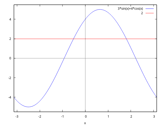
(%i1) load("trigtools")$ (%i2) eq:eq:3*sin(x)+4*cos(x)=2$(%i3) sol:trigsolve(eq,-%pi,%pi); 2 sqrt(21) 12 2 sqrt(21) 12 (%o3) {atan(---------- - --), %pi - atan(---------- + --)} 5 5 5 5(%i4) float(%), numer; (%o4) {- 0.5157783719341241, 1.8027805895206928}Answ. : \(x = \tan^{-1}\left({2\sqrt{21}\over 5} - {12\over 5}\right) + 2\pi k\) ; \(x = \pi - \tan^{-1}\left({2\sqrt{21}\over 5} + {12\over 5}\right) + 2\pi k,\) k – any integer.
-
(%i1) load("trigtools")$(%i2) eq:cos(3*x)-sin(x)=sqrt(3)*(cos(x)-sin(3*x)); (%o2) cos(3 x) - sin(x) = sqrt(3) (cos(x) - sin(3 x))
(%i3) plot2d([lhs(eq)-rhs(eq)], [x,0,2*%pi])$
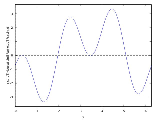
We have 6 solutions from [0, 2*pi].
(%i1) load("trigtools")$ (%i2) eq:cos(3*x)-sin(x)=sqrt(3)*(cos(x)-sin(3*x))$ (%i3) plot2d([lhs(eq)-rhs(eq)], [x,0.2,0.5])$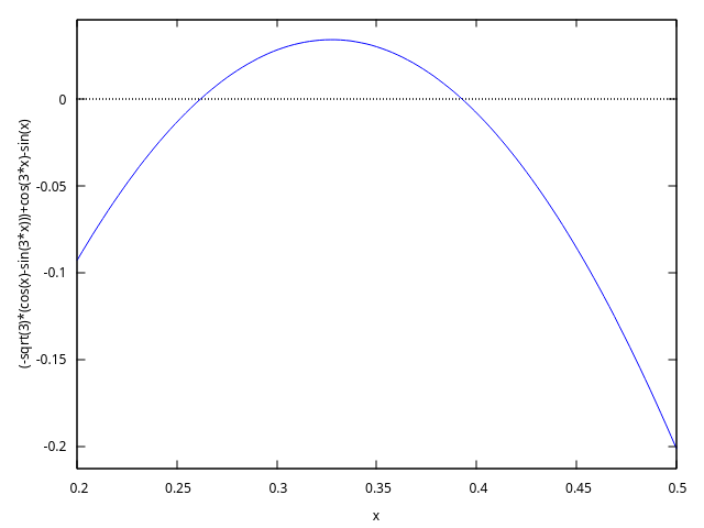
(%i1) load("trigtools")$ (%i2) load("trigtools")$ (%i3) eq:cos(3*x)-sin(x)=sqrt(3)*(cos(x)-sin(3*x))$ (%i4) plot2d([lhs(eq)-rhs(eq)], [x,3.3,3.6])$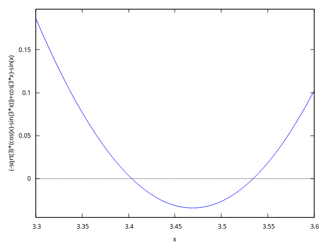
(%i1) load("trigtools")$ (%i2) eq:cos(3*x)-sin(x)=sqrt(3)*(cos(x)-sin(3*x))$(%i3) trigfactor(lhs(eq))=map(trigfactor,rhs(eq)); %pi %pi (%o3) - 2 sin(x + ---) sin(2 x - ---) = 4 4 %pi %pi 2 sqrt(3) sin(x - ---) sin(2 x - ---) 4 4(%i4) factor(lhs(%)-rhs(%)); 4 x + %pi 4 x - %pi (%o4) - 2 (sin(---------) + sqrt(3) sin(---------)) 4 4 8 x - %pi sin(---------) 4Equation is equivalent to
(%i1) load("trigtools")$ (%i2) eq:cos(3*x)-sin(x)=sqrt(3)*(cos(x)-sin(3*x))$(%i3) trigfactor(lhs(eq))=map(trigfactor,rhs(eq)); %pi %pi (%o3) - 2 sin(x + ---) sin(2 x - ---) = 4 4 %pi %pi 2 sqrt(3) sin(x - ---) sin(2 x - ---) 4 4(%i4) L:factor(rhs(%)-lhs(%)); 4 x + %pi 4 x - %pi 8 x - %pi (%o4) 2 (sin(---------) + sqrt(3) sin(---------)) sin(---------) 4 4 4(%i5) eq1:part(L,2)=0; 4 x + %pi 4 x - %pi (%o5) sin(---------) + sqrt(3) sin(---------) = 0 4 4(%i6) eq2:part(L,3)=0; 8 x - %pi (%o6) sin(---------) = 0 4(%i7) S1:trigsolve(eq1,0,2*%pi); %pi 13 %pi (%o7) {---, ------} 12 12(%i8) S2:trigsolve(eq2,0,2*%pi); %pi 5 %pi 9 %pi 13 %pi (%o8) {---, -----, -----, ------} 8 8 8 8(%i9) S:listify(union(S1,S2)); %pi %pi 5 %pi 13 %pi 9 %pi 13 %pi (%o9) [---, ---, -----, ------, -----, ------] 12 8 8 12 8 8(%i10) float(%), numer; (%o10) [0.2617993877991494, 0.39269908169872414, 1.9634954084936207, 3.4033920413889422, 3.5342917352885173, 5.105088062083414]
Answer: \(x = a + 2\pi k,\) where a any from S, k any integer.
-
(%i1) load("trigtools")$(%i2) eq:8*cos(x)*cos(4*x)*cos(5*x)-1=0; (%o2) 8 cos(x) cos(4 x) cos(5 x) - 1 = 0
(%i3) trigrat(%); (%o3) 2 cos(10 x) + 2 cos(8 x) + 2 cos(2 x) + 1 = 0
Left side is periodic with period \(T=\pi.\)
We have 10 solutions from [0, pi].
(%i1) load("trigtools")$ (%i2) eq:8*cos(x)*cos(4*x)*cos(5*x)-1=0$(%i3) plot2d([lhs(eq),rhs(eq)],[x,0,%pi]); (%o3) false
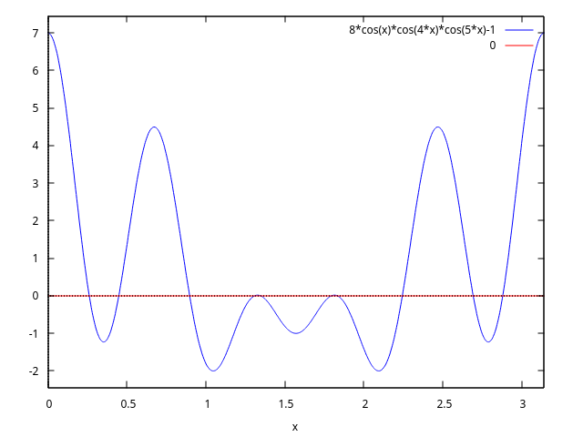
(%i1) load("trigtools")$ (%i2) eq:8*cos(x)*cos(4*x)*cos(5*x)-1=0$(%i3) x4:find_root(eq, x, 1.3, 1.32); (%o3) 1.3089969389957472
(%i4) x5:find_root(eq, x, 1.32, 1.35); (%o4) 1.3463968515384828
(%i5) plot2d([lhs(eq),0], [x,1.3,1.35], [gnuplot_preamble, "set grid;"]); (%o5) false
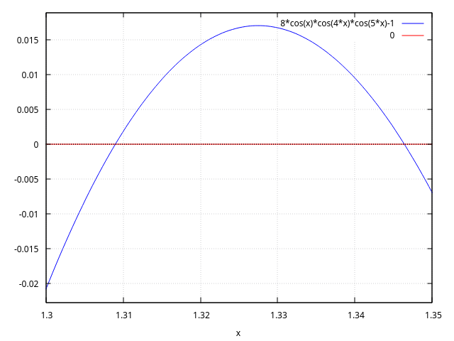
Equation we multiply by \(2\sin x\cos 2x:\)
(%i1) load("trigtools")$ (%i2) eq:8*cos(x)*cos(4*x)*cos(5*x)-1=0$(%i3) eq*2*sin(x)*cos(2*x); (%o3) 2 sin(x) cos(2 x) (8 cos(x) cos(4 x) cos(5 x) - 1) = 0
(%i4) eq1:trigreduce(%),expand; (%o4) sin(13 x) + sin(x) = 0
(%i5) trigfactor(lhs(eq1))=0; (%o5) 2 cos(6 x) sin(7 x) = 0
(%i6) S1:trigsolve(cos(6*x),0,%pi); %pi %pi 5 %pi 7 %pi 3 %pi 11 %pi (%o6) {---, ---, -----, -----, -----, ------} 12 4 12 12 4 12(%i7) S2:trigsolve(sin(7*x),0,%pi); %pi 2 %pi 3 %pi 4 %pi 5 %pi 6 %pi (%o7) {0, ---, -----, -----, -----, -----, -----} 7 7 7 7 7 7We remove solutions of \(\sin x = 0\) and \(\cos 2x = 0.\)
(%i1) load("trigtools")$ (%i2) S1:trigsolve(cos(6*x),0,%pi)$ (%i3) S2:trigsolve(sin(7*x),0,%pi)$(%i4) S3:trigsolve(sin(x),0,%pi); (%o4) {0}(%i5) S4:trigsolve(cos(2*x),0,%pi); %pi 3 %pi (%o5) {---, -----} 4 4We find 10 solutions from \([0, \pi]:\)
(%i1) load("trigtools")$ (%i2) S1:trigsolve(cos(6*x),0,%pi)$ (%i3) S2:trigsolve(sin(7*x),0,%pi)$ (%i4) S3:trigsolve(sin(x),0,%pi)$ (%i5) S4:trigsolve(cos(2*x),0,%pi)$(%i6) union(S1,S2)$ setdifference(%,S3)$ setdifference(%,S4); %pi %pi 2 %pi 5 %pi 3 %pi 4 %pi 7 %pi 5 %pi (%o8) {---, ---, -----, -----, -----, -----, -----, -----, 12 7 7 12 7 7 12 7 6 %pi 11 %pi -----, ------} 7 12(%i9) S:listify(%); %pi %pi 2 %pi 5 %pi 3 %pi 4 %pi 7 %pi 5 %pi (%o9) [---, ---, -----, -----, -----, -----, -----, -----, 12 7 7 12 7 7 12 7 6 %pi 11 %pi -----, ------] 7 12(%i10) length(S); (%o10) 10
(%i11) float(S), numer; (%o11) [0.2617993877991494, 0.4487989505128276, 0.8975979010256552, 1.3089969389957472, 1.3463968515384828, 1.7951958020513104, 1.8325957145940461, 2.243994752564138, 2.6927937030769655, 2.8797932657906435]
Answer: \(x = a + 2\pi k,\) where a any from S, k any integer.
Categories: Trigonometric functions · Package trigtools ·-
Next: Contract atan Functions, Previous: Solve Trigonometric Equations, Up: Functions and Variables for trigtools [Contents][Index]
99.2.6 Evaluation of Trigonometric Functions
- Function: trigvalue (x) 
The function trigvalue compute values of \(\sin {m\pi\over n},\) \(\cos {m\pi\over n},\) \(\tan {m\pi\over n},\) and \(\cot {m\pi\over n}\) in radicals.
trigvalueis essentially an internal function. Use functiontrigevalin preference.load("trigtools")loads this function.
- Function: trigeval (x) 
The function trigeval compute values of expressions with \(\sin {m\pi\over n},\) \(\cos {m\pi\over n},\) \(\tan {m\pi\over n},\) and \(\cot {m\pi\over n}\) in radicals.
load("trigtools") loads this function.
Examples:
- Values of trigonometric functions
(%i1) load("trigtools")$ (%i2) load(trigtools)$(%i3) trigvalue(sin(%pi/10)); sqrt(5) - 1 (%o3) ----------- 4(%i4) trigvalue(cos(%pi/10)); sqrt(sqrt(5) + 5) (%o4) ----------------- 3/2 2(%i5) trigvalue(tan(%pi/10)); sqrt(5 - 2 sqrt(5)) (%o5) ------------------- sqrt(5)(%i6) float(%), numer; (%o6) 0.3249196962329063
(%i7) float(tan(%pi/10)), numer; (%o7) 0.3249196962329063
(%i8) trigvalue(cot(%pi/10)); (%o8) sqrt(2 sqrt(5) + 5)
(%i9) float(%), numer; (%o9) 3.0776835371752536
(%i10) float(cot(%pi/10)), numer; (%o10) 3.077683537175254
(%i11) trigvalue(sin(%pi/32)); sqrt(2 - sqrt(sqrt(sqrt(2) + 2) + 2)) (%o11) ------------------------------------- 2(%i12) trigvalue(cos(%pi/32)); sqrt(sqrt(sqrt(sqrt(2) + 2) + 2) + 2) (%o12) ------------------------------------- 2(%i13) trigvalue(cos(%pi/256)); (%o13) sqrt(sqrt(sqrt(sqrt(sqrt(sqrt(sqrt(2) + 2) + 2) + 2) + 2) + 2) + 2)/2(%i14) trigvalue(cos(%pi/60)); (%o14) sqrt(sqrt(sqrt(2) sqrt(3) sqrt(sqrt(5) + 5) + sqrt(5) + 7) + 4) --------------------------------------------------------------- 3/2 2(%i15) trigvalue(sin(%pi/60)); (%o15) sqrt(4 - sqrt(sqrt(2) sqrt(3) sqrt(sqrt(5) + 5) + sqrt(5) + 7)) --------------------------------------------------------------- 3/2 2(%i16) trigvalue(sin(%pi/18)); %pi (%o16) sin(---) 18(%i17) trigvalue(sin(%pi/20)); sqrt(4 - sqrt(2) sqrt(sqrt(5) + 5)) (%o17) ----------------------------------- 3/2 2 - ode example
(%i1) load("trigtools")$ (%i2) load(odes)$(%i3) eq:'diff(y,x,5)+2*y=0; 5 d y (%o3) --- + 2 y = 0 5 dx(%i4) odeL(eq,y,x); 1/5 4 %pi - 2 cos(-----) x 5 1/5 4 %pi (%o4) y = %e C5 sin(2 sin(-----) x) 5 1/5 4 %pi - 2 cos(-----) x 5 1/5 4 %pi + %e C4 cos(2 sin(-----) x) 5 1/5 2 %pi - 2 cos(-----) x 5 1/5 2 %pi + %e C3 sin(2 sin(-----) x) 5 1/5 2 %pi - 2 cos(-----) x 5 1/5 2 %pi + %e C2 cos(2 sin(-----) x) 5 1/5 - 2 x + %e C1(%i5) sol:trigeval(%); (sqrt(5) - 1) x - --------------- 9/5 2 sqrt(sqrt(5) + 5) x (%o5) y = %e C3 sin(-------------------) 13/10 2 (sqrt(5) - 1) x - --------------- 9/5 2 sqrt(sqrt(5) + 5) x + %e C2 cos(-------------------) 13/10 2 (sqrt(5) + 1) x --------------- 9/5 2 sqrt(5 - sqrt(5)) x + %e C5 sin(-------------------) 13/10 2 (sqrt(5) + 1) x --------------- 9/5 1/5 2 sqrt(5 - sqrt(5)) x - 2 x + %e C4 cos(-------------------) + %e C1 13/10 2(%i6) subst(sol,eq)$ (%i7) ev(%, nouns)$
(%i8) radcan(%); (%o8) 0 = 0
- n-th root of complex number
Example. Find the 4-th roots of %i
(%i1) load("trigtools")$(%i2) solve(x^4=%i,x); 1/8 1/8 1/8 (%o2) [x = (- 1) %i, x = - (- 1) , x = - (- 1) %i, 1/8 x = (- 1) ](%i3) rectform(%); %pi %pi %pi %pi (%o3) [x = %i cos(---) - sin(---), x = - %i sin(---) - cos(---), 8 8 8 8 %pi %pi %pi %pi x = sin(---) - %i cos(---), x = %i sin(---) + cos(---)] 8 8 8 8(%i4) trigeval(%); sqrt(sqrt(2) + 2) %i sqrt(2 - sqrt(2)) (%o4) [x = -------------------- - -----------------, 2 2 sqrt(2 - sqrt(2)) %i sqrt(sqrt(2) + 2) x = - -------------------- - -----------------, 2 2 sqrt(2 - sqrt(2)) sqrt(sqrt(2) + 2) %i x = ----------------- - --------------------, 2 2 sqrt(2 - sqrt(2)) %i sqrt(sqrt(2) + 2) x = -------------------- + -----------------] 2 2
Previous: Evaluation of Trigonometric Functions, Up: Functions and Variables for trigtools [Contents][Index]
99.2.7 Contract atan Functions
- Function: atan_contract (r) 
The function atan_contract(r) contracts atan functions. We assume: \(|r| < {\pi\over 2}.\)
load("trigtools")loads this function.Examples:
-
(%i1) load("trigtools")$(%i2) atan_contract(atan(x)+atan(y)); (%o2) atan(y) + atan(x)
(%i3) assume(abs(atan(x)+atan(y))<%pi/2)$
(%i4) atan(x)+atan(y)=atan_contract(atan(x)+atan(y)); y + x (%o4) atan(y) + atan(x) = atan(-------) 1 - x y -
(%i1) load("trigtools")$(%i2) atan(1/3)+atan(1/5)+atan(1/7)+atan(1/8)$ %=atan_contract(%); 1 1 1 1 %pi (%o3) atan(-) + atan(-) + atan(-) + atan(-) = --- 3 5 7 8 4 - Machin’s formulae
(%i1) load("trigtools")$(%i2) 4*atan(1/5)-atan(1/239)=atan_contract(4*atan(1/5)-atan(1/239)); 1 1 %pi (%o2) 4 atan(-) - atan(---) = --- 5 239 4 - see https://en.wikipedia.org/wiki/Machin-like_formula
(%i1) load("trigtools")$ (%i2) 12*atan(1/49)+32*atan(1/57)-5*atan(1/239)+12*atan(1/110443)$(%i3) %=atan_contract(%); 1 1 1 (%o3) 12 atan(--) + 32 atan(--) - 5 atan(---) 49 57 239 1 %pi + 12 atan(------) = --- 110443 4
Categories: Trigonometric functions · Package trigtools ·-
Previous: Functions and Variables for trigtools, Up: Package trigtools [Contents][Index]
99.3 References
Next: Package wrstcse, Previous: Package trigtools [Contents][Index]
100 Package unit
Next: Functions and Variables for Units, Previous: Package unit, Up: Package unit [Contents][Index]
100.1 Introduction to Units
The unit package enables the user to convert between arbitrary units and work with dimensions in equations. The functioning of this package is radically different from the original Maxima units package - whereas the original was a basic list of definitions, this package uses rulesets to allow the user to chose, on a per dimension basis, what unit final answers should be rendered in. It will separate units instead of intermixing them in the display, allowing the user to readily identify the units associated with a particular answer. It will allow a user to simplify an expression to its fundamental Base Units, as well as providing fine control over simplifying to derived units. Dimensional analysis is possible, and a variety of tools are available to manage conversion and simplification options. In addition to customizable automatic conversion, units also provides a traditional manual conversion option.
Note - when unit conversions are inexact Maxima will make approximations resulting in fractions. This is a consequence of the techniques used to simplify units. The messages warning of this type of substitution are disabled by default in the case of units (normally they are on) since this situation occurs frequently and the warnings clutter the output. (The existing state of ratprint is restored after unit conversions, so user changes to that setting will be preserved otherwise.) If the user needs this information for units, they can set unitverbose:on to reactivate the printing of warnings from the unit conversion process.
unit is included in Maxima in the share/contrib/unit directory. It obeys normal Maxima package loading conventions:
(%i1) load("unit")$
*******************************************************************
* Units version 0.50 *
* Definitions based on the NIST Reference on *
* Constants, Units, and Uncertainty *
* Conversion factors from various sources including *
* NIST and the GNU units package *
*******************************************************************
Redefining necessary functions...
WARNING: DEFUN/DEFMACRO: redefining function TOPLEVEL-MACSYMA-EVAL ...
WARNING: DEFUN/DEFMACRO: redefining function MSETCHK ...
WARNING: DEFUN/DEFMACRO: redefining function KILL1 ...
WARNING: DEFUN/DEFMACRO: redefining function NFORMAT ...
Initializing unit arrays...
Done.
The WARNING messages are expected and not a cause for concern - they indicate the unit package is redefining functions already defined in Maxima proper. This is necessary in order to properly handle units. The user should be aware that if other changes have been made to these functions by other packages those changes will be overwritten by this loading process.
The unit.mac file also loads a lisp file unit-functions.lisp which contains the lisp functions needed for the package.
Clifford Yapp is the primary author. He has received valuable assistance from Barton Willis of the University of Nebraska at Kearney (UNK), Robert Dodier, and other intrepid folk of the Maxima mailing list.
There are probably lots of bugs. Let me know. float and numer
don’t do what is expected.
TODO : dimension functionality, handling of temperature, showabbr and friends. Show examples with addition of quantities containing units.
Previous: Introduction to Units, Up: Package unit [Contents][Index]
100.2 Functions and Variables for Units
- Function: setunits (list) 
By default, the unit package does not use any derived dimensions, but will convert all units to the seven fundamental dimensions using MKS units.
(%i2) N; kg m (%o2) ---- 2 s(%i3) dyn; 1 kg m (%o3) (------) (----) 100000 2 s(%i4) g; 1 (%o4) (----) (kg) 1000(%i5) centigram*inch/minutes^2; 127 kg m (%o5) (-------------) (----) 1800000000000 2 sIn some cases this is the desired behavior. If the user wishes to use other units, this is achieved with the
setunitscommand:(%i6) setunits([centigram,inch,minute]); (%o6) done
(%i7) N; 1800000000000 %in cg (%o7) (-------------) (------) 127 2 %min(%i8) dyn; 18000000 %in cg (%o8) (--------) (------) 127 2 %min(%i9) g; (%o9) (100) (cg)
(%i10) centigram*inch/minutes^2; %in cg (%o10) ------ 2 %minThe setting of units is quite flexible. For example, if we want to get back to kilograms, meters, and seconds as defaults for those dimensions we can do:
(%i11) setunits([kg,m,s]); (%o11) done
(%i12) centigram*inch/minutes^2; 127 kg m (%o12) (-------------) (----) 1800000000000 2 sDerived units are also handled by this command:
(%i17) setunits(N); (%o17) done
(%i18) N; (%o18) N
(%i19) dyn; 1 (%o19) (------) (N) 100000(%i20) kg*m/s^2; (%o20) N
(%i21) centigram*inch/minutes^2; 127 (%o21) (-------------) (N) 1800000000000Notice that the unit package recognized the non MKS combination of mass, length, and inverse time squared as a force, and converted it to Newtons. This is how Maxima works in general. If, for example, we prefer dyne to Newtons, we simply do the following:
(%i22) setunits(dyn); (%o22) done
(%i23) kg*m/s^2; (%o23) (100000) (dyn)
(%i24) centigram*inch/minutes^2; 127 (%o24) (--------) (dyn) 18000000To discontinue simplifying to any force, we use the uforget command:
(%i26) uforget(dyn); (%o26) false
(%i27) kg*m/s^2; kg m (%o27) ---- 2 s(%i28) centigram*inch/minutes^2; 127 kg m (%o28) (-------------) (----) 1800000000000 2 sThis would have worked equally well with
uforget(N)oruforget(%force).See also
uforget. To use this function write firstload("unit").Categories: Package unit ·
- Function: uforget (list) 
By default, the unit package converts all units to the seven fundamental dimensions using MKS units. This behavior can be changed with the
setunitscommand. After that, the user can restore the default behavior for a particular dimension by means of theuforgetcommand:(%i13) setunits([centigram,inch,minute]); (%o13) done
(%i14) centigram*inch/minutes^2; %in cg (%o14) ------ 2 %min(%i15) uforget([cg,%in,%min]); (%o15) [false, false, false]
(%i16) centigram*inch/minutes^2; 127 kg m (%o16) (-------------) (----) 1800000000000 2 suforgetoperates on dimensions, not units, so any unit of a particular dimension will work. The dimension itself is also a legal argument.See also
setunits. To use this function write firstload("unit").Categories: Package unit ·
- Function: convert (expr, list) 
When resetting the global environment is overkill, there is the
convertcommand, which allows one time conversions. It can accept either a single argument or a list of units to use in conversion. When a convert operation is done, the normal global evaluation system is bypassed, in order to avoid the desired result being converted again. As a consequence, for inexact calculations "rat" warnings will be visible if the global environment controlling this behavior (ratprint) is true. This is also useful for spot-checking the accuracy of a global conversion. Another feature isconvertwill allow a user to do Base Dimension conversions even if the global environment is set to simplify to a Derived Dimension.(%i2) kg*m/s^2; kg m (%o2) ---- 2 s(%i3) convert(kg*m/s^2,[g,km,s]); g km (%o3) ---- 2 s(%i4) convert(kg*m/s^2,[g,inch,minute]); `rat' replaced 39.37007874015748 by 5000/127 = 39.37007874015748 18000000000 %in g (%o4) (-----------) (-----) 127 2 %min(%i5) convert(kg*m/s^2,[N]); (%o5) N
(%i6) convert(kg*m^2/s^2,[N]); (%o6) m N
(%i7) setunits([N,J]); (%o7) done
(%i8) convert(kg*m^2/s^2,[N]); (%o8) m N
(%i9) convert(kg*m^2/s^2,[N,inch]); `rat' replaced 39.37007874015748 by 5000/127 = 39.37007874015748 5000 (%o9) (----) (%in N) 127(%i10) convert(kg*m^2/s^2,[J]); (%o10) J
(%i11) kg*m^2/s^2; (%o11) J
(%i12) setunits([g,inch,s]); (%o12) done
(%i13) kg*m/s^2; (%o13) N
(%i14) uforget(N); (%o14) false
(%i15) kg*m/s^2; 5000000 %in g (%o15) (-------) (-----) 127 2 s(%i16) convert(kg*m/s^2,[g,inch,s]); `rat' replaced 39.37007874015748 by 5000/127 = 39.37007874015748 5000000 %in g (%o16) (-------) (-----) 127 2 sSee also
setunitsanduforget. To use this function write firstload("unit").Categories: Package unit ·
- Optional variable: usersetunits 
Default value: none
If a user wishes to have a default unit behavior other than that described, they can make use of maxima-init.mac and the usersetunits variable. The unit package will check on startup to see if this variable has been assigned a list. If it has, it will use setunits on that list and take the units from that list to be defaults.
uforgetwill revert to the behavior defined by usersetunits over its own defaults. For example, if we have a maxima-init.mac file containing:usersetunits : [N,J];
we would see the following behavior:
(%i1) load("unit")$ ******************************************************************* * Units version 0.50 * * Definitions based on the NIST Reference on * * Constants, Units, and Uncertainty * * Conversion factors from various sources including * * NIST and the GNU units package * ******************************************************************* Redefining necessary functions... WARNING: DEFUN/DEFMACRO: redefining function TOPLEVEL-MACSYMA-EVAL ... WARNING: DEFUN/DEFMACRO: redefining function MSETCHK ... WARNING: DEFUN/DEFMACRO: redefining function KILL1 ... WARNING: DEFUN/DEFMACRO: redefining function NFORMAT ... Initializing unit arrays... Done. User defaults found... User defaults initialized.(%i2) kg*m/s^2; (%o2) N
(%i3) kg*m^2/s^2; (%o3) J
(%i4) kg*m^3/s^2; (%o4) J m
(%i5) kg*m*km/s^2; (%o5) (1000) (J)
(%i6) setunits([dyn,eV]); (%o6) done
(%i7) kg*m/s^2; (%o7) (100000) (dyn)
(%i8) kg*m^2/s^2; (%o8) (6241509596477042688) (eV)
(%i9) kg*m^3/s^2; (%o9) (6241509596477042688) (eV m)
(%i10) kg*m*km/s^2; (%o10) (6241509596477042688000) (eV)
(%i11) uforget([dyn,eV]); (%o11) [false, false]
(%i12) kg*m/s^2; (%o12) N
(%i13) kg*m^2/s^2; (%o13) J
(%i14) kg*m^3/s^2; (%o14) J m
(%i15) kg*m*km/s^2; (%o15) (1000) (J)
Without
usersetunits, the initial inputs would have been converted to MKS, and uforget would have resulted in a return to MKS rules. Instead, the user preferences are respected in both cases. Notice these can still be overridden if desired. To completely eliminate this simplification - i.e. to have the user defaults reset to factory defaults - thedontusedimensioncommand can be used.uforgetcan restore user settings again, but only ifusedimensionfrees it for use. Alternately,kill(usersetunits)will completely remove all knowledge of the user defaults from the session. Here are some examples of how these various options work.(%i2) kg*m/s^2; (%o2) N
(%i3) kg*m^2/s^2; (%o3) J
(%i4) setunits([dyn,eV]); (%o4) done
(%i5) kg*m/s^2; (%o5) (100000) (dyn)
(%i6) kg*m^2/s^2; (%o6) (6241509596477042688) (eV)
(%i7) uforget([dyn,eV]); (%o7) [false, false]
(%i8) kg*m/s^2; (%o8) N
(%i9) kg*m^2/s^2; (%o9) J
(%i10) dontusedimension(N); (%o10) [%force]
(%i11) dontusedimension(J); (%o11) [%energy, %force]
(%i12) kg*m/s^2; kg m (%o12) ---- 2 s(%i13) kg*m^2/s^2; 2 kg m (%o13) ----- 2 s(%i14) setunits([dyn,eV]); (%o14) done
(%i15) kg*m/s^2; kg m (%o15) ---- 2 s(%i16) kg*m^2/s^2; 2 kg m (%o16) ----- 2 s(%i17) uforget([dyn,eV]); (%o17) [false, false]
(%i18) kg*m/s^2; kg m (%o18) ---- 2 s(%i19) kg*m^2/s^2; 2 kg m (%o19) ----- 2 s(%i20) usedimension(N); Done. To have Maxima simplify to this dimension, use setunits([unit]) to select a unit. (%o20) true
(%i21) usedimension(J); Done. To have Maxima simplify to this dimension, use setunits([unit]) to select a unit. (%o21) true
(%i22) kg*m/s^2; kg m (%o22) ---- 2 s(%i23) kg*m^2/s^2; 2 kg m (%o23) ----- 2 s(%i24) setunits([dyn,eV]); (%o24) done
(%i25) kg*m/s^2; (%o25) (100000) (dyn)
(%i26) kg*m^2/s^2; (%o26) (6241509596477042688) (eV)
(%i27) uforget([dyn,eV]); (%o27) [false, false]
(%i28) kg*m/s^2; (%o28) N
(%i29) kg*m^2/s^2; (%o29) J
(%i30) kill(usersetunits); (%o30) done
(%i31) uforget([dyn,eV]); (%o31) [false, false]
(%i32) kg*m/s^2; kg m (%o32) ---- 2 s(%i33) kg*m^2/s^2; 2 kg m (%o33) ----- 2 sUnfortunately this wide variety of options is a little confusing at first, but once the user grows used to them they should find they have very full control over their working environment.
Categories: Package unit ·
- Function: metricexpandall (x) 
Rebuilds global unit lists automatically creating all desired metric units. x is a numerical argument which is used to specify how many metric prefixes the user wishes defined. The arguments are as follows, with each higher number defining all lower numbers’ units:
0 - none. Only base units 1 - kilo, centi, milli (default) 2 - giga, mega, kilo, hecto, deka, deci, centi, milli, micro, nano 3 - peta, tera, giga, mega, kilo, hecto, deka, deci, centi, milli, micro, nano, pico, femto 4 - allNormally, Maxima will not define the full expansion since this results in a very large number of units, but
metricexpandallcan be used to rebuild the list in a more or less complete fashion. The relevant variable in the unit.mac file is %unitexpand.Categories: Package unit ·
- Variable: %unitexpand 
Default value:
2This is the value supplied to
metricexpandallduring the initial loading of unit.Categories: Package unit ·
Next: Package zeilberger, Previous: Package unit [Contents][Index]
101 Package wrstcse
Next: Functions and Variables for wrstcse, Previous: Package wrstcse, Up: Package wrstcse [Contents][Index]
101.1 Introduction to wrstcse
wrstcse provides a few approaches to worst case calculations that are powerful enough
for most engineering problems, but avoid the problems that make a true interval arithmetic
unfeasible for non-trivial problems:
- Extreme worst case calculation by determining which combination of
extreme input values will yield the most extreme result
(
wc_mintypmax,wc_systematic). Its approach isn’t guaranteed to find local minima and maxima in the middle of the input parameter space. In most real-world problems, though, the derivation of the result to each parameter doesn’t change its sign in the tolerance space, which moves the extreme cases to the edges of the tolerance space making them accessible to this method. Viawc_ewc_simplifythis method can typically be reduced from a brute-force approach to being O(n)-complete. - The monte carlo approach that assigns each parameter random values in the tolerance space and, when repeated n times will yield a view of the distribution n samples might have. The view provided by this method is pessimistic, as most real-wprld items are more probabible to lie in the middle of the tolerance space than at its end.
- The root mean square approach that knowing an approximation of the
parameters of the gaussian distribution of the input values one can
determine how big the tolerances will realistically be if one requires
a given yield (see
wc_mintypmax_rss). Note that even rectangles tend to quickly add up to approximation of gauss curve, if affecting the same tolerance which makes this method applicable to most real-world problems.
Tolerances are applied to parameters by providing each tolerance-laden parameter with a tol[n] that wrstcase will vary between -1 and 1 looking for extreme results, while rol[n]=0 should yield the typical value of a parameter.. Using the same n for two parameters will make both parameters have coupled tolerances. Therefore two 1% resistors that both will change over the temperature range by another 2% in the same way can be defined as follows:
(%i1) load("wrstcse")$
(%i2) vals: [
R_1= 1000.0*(1+tol[1]*.01)*(1+tol[3]*.02),
R_2= 2000.0*(1+tol[2]*.01)*(1+tol[3]*.02)
];
(%o2) [R_1 = 1000.0 (0.01 tol + 1) (0.02 tol + 1),
1 3
R_2 = 2000.0 (0.01 tol + 1) (0.02 tol + 1)]
2 3
(%i3) R_1+R_2=wc_mintypmax(subst(vals,R_1+R_2));
(%o3) R_2 + R_1 = [min = 2910.6, typ = 3000.0,
max = 3090.6000000000004]
(%i4) R_1+R_2=wc_mintypmax_percent(subst(vals,R_1+R_2));
(%o4) R_2 + R_1 = [min = - 2.980000000000005 %, typ = 3000.0,
max = 3.0200000000000227 %]
(%i5) R_1/R_2=wc_mintypmax(subst(vals,R_1/R_2));
R_1
(%o5) --- = [min = 0.4900990099009901, typ = 0.5,
R_2
max = 0.5101010101010102]
(%i6) R_1/R_2=wc_mintypmax_percent(subst(vals,R_1/R_2));
R_1
(%o6) --- = [min = - 1.980198019801982 %, typ = 0.5,
R_2
max = 2.020202020202033 %]
load ("wrstcse") loads this package.
Previous: Introduction to wrstcse, Up: Package wrstcse [Contents][Index]
101.2 Functions and Variables for wrstcse
- Function: wc_typicalvalues (expression) 
-
Returns what happens if all tol[n] happen to be 0, which moves all parameter to the middle of their tolerance range.
Example:
(%i1) load("wrstcse")$(%i2) vals: [ R_1= 1000.0*(1+tol[1]*.01), R_2= 2000.0*(1+tol[2]*.01) ]; (%o2) [R_1 = 1000.0 (0.01 tol + 1), 1 R_2 = 2000.0 (0.01 tol + 1)] 2(%i3) divider:U_Out=U_In*R_1/(R_1+R_2); R_1 U_In (%o3) U_Out = --------- R_2 + R_1(%i4) wc_typicalvalues(vals); (%o4) [R_1 = 1000.0, R_2 = 2000.0]
(%i5) wc_typicalvalues(subst(vals,divider)); (%o5) U_Out = 0.3333333333333333 U_In
- Function: wc_inputvalueranges (expression, [show_tols]) 
-
Convenience function: Displays a list which parameter can vary between which values.
If show_tols is
truethen this function additionally displays which tol[n] each variable is affected by.See also
wc_mintypmax2tolandwc_inputvalueassumptions.Example:
(%i1) load("wrstcse")$(%i2) vals: [ R_1= 1000.0*(1+tol["R_1"]*.01+tol["Temp"]*.001), R_2= 2000.0*(1+tol["R_2"]*.01+tol["Temp"]*.001), R_3= 2000.0*(1+tol["R_3"]*.01) ]; (%o2) [R_1 = 1000.0 (0.001 tol + 0.01 tol + 1), Temp R_1 R_2 = 2000.0 (0.001 tol + 0.01 tol + 1), Temp R_2 R_3 = 2000.0 (0.01 tol + 1)] R_3(%i3) wc_inputvalueranges(vals); (%o3) [ R_1 min = 989.0 typ = 1000.0 max = 1010.9999999999999 ] [ ] [ R_2 min = 1978.0 typ = 2000.0 max = 2021.9999999999998 ] [ ] [ R_3 min = 1980.0 typ = 2000.0 max = 2020.0 ](%i4) wc_inputvalueranges(vals,true); [ R_1 ] [ min = 989.0 ] [ ] [ ] (%o4) Col 1 = [ R_2 ] Col 2 = [ min = 1978.0 ] [ ] [ ] [ R_3 ] [ min = 1980.0 ] [ typ = 1000.0 ] [ max = 1010.9999999999999 ] [ ] [ ] Col 3 = [ typ = 2000.0 ] Col 4 = [ max = 2021.9999999999998 ] [ ] [ ] [ typ = 2000.0 ] [ max = 2020.0 ] [ [tol , tol ] ] [ Temp R_1 ] [ ] Col 5 = [ [tol , tol ] ] [ Temp R_2 ] [ ] [ [tol ] ] [ R_3 ]
- Function: wc_systematic (expression, [num]) 
-
Systematically introduces num values per parameter into expression and returns a list of the result. If no num is given, num defaults to wc_defaultvaluespertol. Negative values for num make
wc_systematicuse the monte carlo method with num samples, instead.If an equation uses the following values with tolerances:
vals:[R_1=100+tol[1],R_2=100+tol[2]];num=2will cause the following combinations of tolerances to be tested: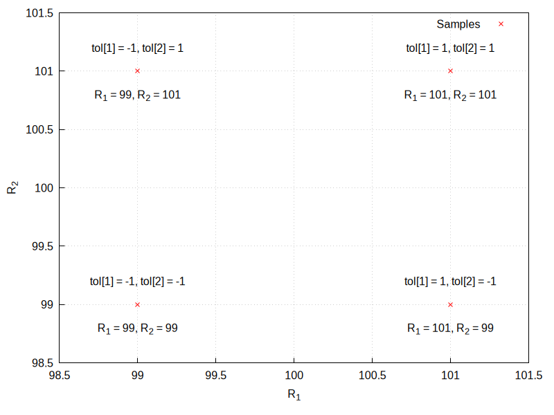
num=3will cause the following combinations of tolerances to be tested: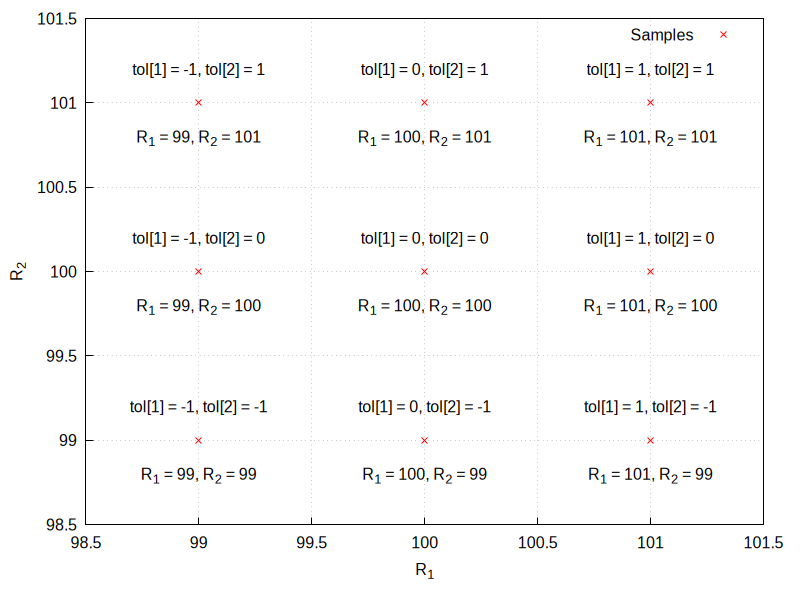
num=-500will cause the following combinations of tolerances to be tested, instead: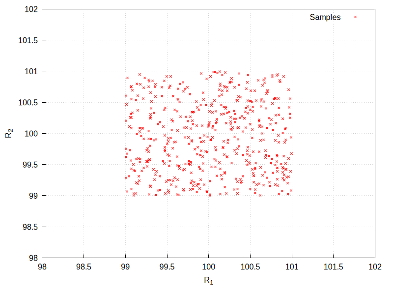
See also
wc_defaultvaluespertol,wc_mintypmax,wc_defaultvaluespertol,wc_ewc_simplifyandwc_montecarlo.Example:
(%i1) load("wrstcse")$(%i2) vals: [ R_1= 1000.0*(1+tol[1]*.01), R_2= 2000.0*(1+tol[2]*.01) ]; (%o2) [R_1 = 1000.0 (0.01 tol + 1), 1 R_2 = 2000.0 (0.01 tol + 1)] 2(%i3) divider: U_Out=U_In*(R_1)/(R_1+R_2); R_1 U_In (%o3) U_Out = --------- R_2 + R_1(%i4) wc_systematic(subst(vals,rhs(divider))); (%o4) [0.33333333333333337 U_In, 0.3311036789297659 U_In, 0.3289036544850498 U_In, 0.3355704697986577 U_In, 0.3333333333333333 U_In, 0.33112582781456956 U_In, 0.3377926421404682 U_In, 0.3355481727574751 U_In, 0.3333333333333333 U_In]
- Function: wc_ewc_simplify (expression, definitions...) 
-
Brute-forcing through all combinations of tol[n] in order to find the worst-case combination is O(m^n)-complete and therefore computationally intensive for high numbers of tol[n].
wc_ewc_simplifyuses the sign of the derivatives of expression to combine as manytol[n], as possible. The result is an expression that might run much faster throughwc_mintypmaxandwc_systematic, but that, if the derivate of expression doesn’t change sign in the tol[n] space, still yields the same results for the brute-force approaches to worst-case analysis.Note that changing the number of tol[n] will change the statistical distribution of the results over the tol[n] space and therefore will change the statistical distribution of the montecarlo method and the results of the root sum square functions.
See also
wc_mintypmaxandwc_montecarlo.definitions allows to temporarily asssign values to specific tol[n] during the optimizations (normally optimizagion is done with all tol[n] being zero) which has the side-effect of excempting these tol[n] from the optimization.
Example:
(%i1) load("wrstcse")$(%i2) vals: [ R_1= 1000.0*(1+tol[1]*.01), R_2= 2000.0*(1+tol[2]*.01) ]; (%o2) [R_1 = 1000.0 (0.01 tol + 1), 1 R_2 = 2000.0 (0.01 tol + 1)] 2(%i3) ratprint:false; (%o3) false
(%i4) assume(U_In>0); (%o4) [U_In > 0]
(%i5) divider: U_Out=U_In*(R_1)/(R_1+R_2); R_1 U_In (%o5) U_Out = --------- R_2 + R_1(%i6) divider_vals:subst(vals,divider); 1000.0 (0.01 tol + 1) U_In 1 (%o6) U_Out = ----------------------------------------------- 2000.0 (0.01 tol + 1) + 1000.0 (0.01 tol + 1) 2 1(%i7) divider_vals_simplified:lhs(divider_vals)=wc_ewc_simplify(rhs(divider_vals)); 1000.0 (1 - 0.01 tol ) U_In 2 (%o7) U_Out = ----------------------------------------------- 2000.0 (0.01 tol + 1) + 1000.0 (1 - 0.01 tol ) 2 2(%i8) wc_systematic(rhs(divider_vals)); (%o8) [0.33333333333333337 U_In, 0.3311036789297659 U_In, 0.3289036544850498 U_In, 0.3355704697986577 U_In, 0.3333333333333333 U_In, 0.33112582781456956 U_In, 0.3377926421404682 U_In, 0.3355481727574751 U_In, 0.3333333333333333 U_In]
(%i9) wc_systematic(rhs(divider_vals_simplified)); (%o9) [0.3377926421404682 U_In, 0.3333333333333333 U_In, 0.3289036544850498 U_In](%i10) lhs(divider_vals)=wc_mintypmax(rhs(divider_vals)); (%o10) U_Out = [min = 0.3289036544850498 U_In, typ = 0.3333333333333333 U_In, max = 0.3377926421404682 U_In](%i11) lhs(divider_vals_simplified)=wc_mintypmax(rhs(divider_vals_simplified)); (%o11) U_Out = [min = 0.3289036544850498 U_In, typ = 0.3333333333333333 U_In, max = 0.3377926421404682 U_In]Use case for adding definitions (tol["E_Gain"] cannot be optimized without knowing the sign of tol["U_In"]):
(%i1) load("wrstcse")$(%i2) vals: [ U_In=1.2*tol["U_In"], /* The input voltage range */ n_Bits=16, /* The ADC's number of bits */ U_Ref=1.2*(1+.01*tol["U_Ref"]), /* The Adc's reference */ E_Gain=1+1.2e-6*tol["E_Gain"], /* Gain error */ E_Offset=1.5e-6 /* Offset error */ ]; (%o2) [U_In = 1.2 tol , n_Bits = 16, U_In U_Ref = 1.2 (0.01 tol + 1), E_Gain = 1.2e-6 tol + 1, U_Ref E_Gain E_Offset = 1.5e-6](%i3) ratprint:false; (%o3) false
(%i4) wc_inputvalueranges(vals); (%o4) [ U_In min = - 1.2 typ = 0 max = 1.2 ] [ ] [ n_Bits min = 16 typ = 16 max = 16 ] [ ] [ U_Ref min = 1.188 typ = 1.2 max = 1.212 ] [ ] [ E_Gain min = 0.9999988 typ = 1 max = 1.0000012 ] [ ] [ E_Offset min = 1.5e-6 typ = 1.5e-6 max = 1.5e-6 ](%i5) ndsadc:n_DSADC=((U_In*E_Gain+E_Offset)/U_Ref+.5)*(2^(n_Bits)-1); n_Bits E_Gain U_In + E_Offset (%o5) n_DSADC = (2 - 1) (---------------------- + 0.5) U_Ref(%i6) lhs(ndsadc)=wc_ewc_simplify(subst(vals,rhs(ndsadc))); (%o6) n_DSADC = 65535 ((0.8333333333333334 (1.5e-6 - 1.2 (1.2e-6 tol + 1) tol )) E_Gain U_Ref /(0.01 tol + 1) + 0.5) U_Ref(%i7) lhs(ndsadc)=wc_ewc_simplify(subst(vals,rhs(ndsadc)),tol["U_In"]=1); (%o7) n_DSADC = 65535 ((0.8333333333333334 (1.2 tol (1 - 1.2e-6 tol ) + 1.5e-6)) U_In U_Ref /(0.01 tol + 1) + 0.5) U_Ref
- Function: wc_montecarlo (expression, num) 
-
Introduces num random values per parameter into expression and returns a list of the result.
See also
wc_systematic.Example:
(%i1) load("wrstcse")$(%i2) vals: [ R_1= 1000.0*(1+tol[1]*.01), R_2= 2000.0*(1+tol[2]*.01) ]; (%o2) [R_1 = 1000.0 (0.01 tol + 1), 1 R_2 = 2000.0 (0.01 tol + 1)] 2(%i3) divider: U_Out=U_In*(R_1)/(R_1+R_2); R_1 U_In (%o3) U_Out = --------- R_2 + R_1(%i4) wc_montecarlo(subst(vals,rhs(divider)),10); (%o4) [0.3301505377099377 U_In, 0.33276843198354916 U_In, 0.33406203454153227 U_In, 0.33434833585190965 U_In, 0.3341006856369802 U_In, 0.3359647531928058 U_In, 0.32911646313213117 U_In, 0.333158315034511 U_In, 0.3325173140803672 U_In, 0.3331108406798784 U_In]
- Function: wc_mintypmax (expr, [n]) 
-
Prints the minimum, maximum and typical value of expr. If n is positive, n values for each parameter will be tried systematically. If n is negative, -n random values are used instead. If no n is given, wc_defaultvaluespertol is assumed.
See also
wc_mintypmax_percent,wc_mintypmax_rss,wc_ewc_simplifyandwc_systematic.Example:
(%i1) load("wrstcse")$ (%i2) ratprint:false$(%i3) vals: [ R_1= 1000.0*(1+tol[1]*.01), R_2= 1000.0*(1+tol[2]*.01) ]; (%o3) [R_1 = 1000.0 (0.01 tol + 1), 1 R_2 = 1000.0 (0.01 tol + 1)] 2(%i4) assume(U_In>0); (%o4) [U_In > 0]
(%i5) divider:U_Out=U_In*R_1/(R_1+R_2); R_1 U_In (%o5) U_Out = --------- R_2 + R_1(%i6) lhs(divider)=wc_mintypmax(subst(vals,rhs(divider))); (%o6) U_Out = [min = 0.495 U_In, typ = 0.5 U_In, max = 0.505 U_In]
- Function: wc_mintypmax_percent (expr, sigmas) 
-
Like
wc_mintypmax, but outputs the tolerance range in percent.See
wc_mintypmax.Example:
(%i1) load("wrstcse")$ (%i2) ratprint:false$ (%i3) wc_defaultsigma:6$(%i4) vals: [ R_1= 1000.0*(1+tol[1]*.01), R_2= 1000.0*(1+tol[2]*.01) ]; (%o4) [R_1 = 1000.0 (0.01 tol + 1), 1 R_2 = 1000.0 (0.01 tol + 1)] 2(%i5) assume(U_In>0); (%o5) [U_In > 0]
(%i6) divider:U_Out=U_In*R_1/(R_1+R_2); R_1 U_In (%o6) U_Out = --------- R_2 + R_1(%i7) lhs(divider)=wc_mintypmax(subst(vals,rhs(divider))); (%o7) U_Out = [min = 0.495 U_In, typ = 0.5 U_In, max = 0.505 U_In](%i8) lhs(divider)=wc_mintypmax_percent(subst(vals,rhs(divider))); (%o8) U_Out = [min = - 1.0000000000000009 %, typ = 0.5 U_In, max = 1.0000000000000009 %]
- Function: wc_mintypmax_rss (expr, sigmas) 
-
Prints the minimum and maximum of expr, as well as how high the probability is that expr will lie out of that range based on a root sum square calculation and assuming all input ranges will be gauss-shaped.
wc_defaultsigma defines how many sigma of an input value’s tolerance distribution the range of tol[n]=[-1...1] corresponds to.
The RSS methods has a few advantages a brute-force worst-case calculation: It is fast even witput
wc_ewc_simplify. It prevents overengineering resulting from assuming all tolerances to add up in a catastrophical way if this only happens in a neglectible number of cases. But it will yield only the correct results if the gaussian distribution of the input data is known.Due to its nature this method doesn’t support tolerances that aren’t symmetrical. Therefore in that case the tolerances are extended in the direction that is less wide.
See also
wc_defaultsigmawc_mintypmax_rss_percent, andwc_mintypmax.Example:
(%i1) load("wrstcse")$ (%i2) ratprint:false$ (%i3) wc_defaultsigma:6$(%i4) vals: [ R_1= 1000.0*(1+tol[1]*.01), R_2= 1000.0*(1+tol[2]*.01) ]; (%o4) [R_1 = 1000.0 (0.01 tol + 1), 1 R_2 = 1000.0 (0.01 tol + 1)] 2(%i5) assume(U_In>0); (%o5) [U_In > 0]
(%i6) divider:U_Out=U_In*R_1/(R_1+R_2); R_1 U_In (%o6) U_Out = --------- R_2 + R_1(%i7) lhs(divider)=wc_mintypmax_rss(subst(vals,rhs(divider)),6); (%o7) U_Out = [min = 0.49646446609406725 U_In, typ = 0.5 U_In, max = 0.5035355339059328 U_In, Fail = 0.0019731752898266564 ppm]
- Function: wc_mintypmax_rss_percent (expr, sigmas) 
-
Like
wc_mintypmax_rss, but outputs the tolerance range in percent.See
wc_mintypmax_rss.Example:
(%i1) load("wrstcse")$ (%i2) ratprint:false$ (%i3) wc_defaultsigma:6$(%i4) vals: [ R_1= 1000.0*(1+tol[1]*.01), R_2= 1000.0*(1+tol[2]*.01) ]; (%o4) [R_1 = 1000.0 (0.01 tol + 1), 1 R_2 = 1000.0 (0.01 tol + 1)] 2(%i5) assume(U_In>0); (%o5) [U_In > 0]
(%i6) divider:U_Out=U_In*R_1/(R_1+R_2); R_1 U_In (%o6) U_Out = --------- R_2 + R_1(%i7) lhs(divider)=wc_mintypmax_rss(subst(vals,rhs(divider)),6); (%o7) U_Out = [min = 0.49646446609406725 U_In, typ = 0.5 U_In, max = 0.5035355339059328 U_In, Fail = 0.0019731752898266564 ppm]
(%i8) lhs(divider)=float(wc_mintypmax_rss_percent(subst(vals,rhs(divider)),6)); (%o8) U_Out = [min = - 0.7071067811865506 %, typ = 0.5 U_In, max = 0.7071067811865506 %, Fail = 0.0019731752898266564 ppm]
- Option variable: wc_defaultsigma 
Default value:
6Defines how many sigmas of the gauss distribution that represents the tolerances of a parameter correspond to a tol[n] value of -1...1.
See also
wc_mintypmax_rss.Example:
(%i1) load("wrstcse")$ (%i2) ratprint:false$(%i3) vals: [ R_1= 1000.0*(1+tol[1]*.01), R_2= 1000.0*(1+tol[2]*.01) ]; (%o3) [R_1 = 1000.0 (0.01 tol + 1), 1 R_2 = 1000.0 (0.01 tol + 1)] 2(%i4) assume(U_In>0); (%o4) [U_In > 0]
(%i5) divider:U_Out=U_In*R_1/(R_1+R_2); R_1 U_In (%o5) U_Out = --------- R_2 + R_1(%i6) wc_defaultsigma:1$
(%i7) lhs(divider)=wc_mintypmax_rss(subst(vals,rhs(divider)),6); (%o7) U_Out = [min = 0.4787867965644036 U_In, typ = 0.5 U_In, max = 0.5212132034355964 U_In, Fail = 0.0019731752898266564 ppm]
(%i8) wc_defaultsigma:3$
(%i9) lhs(divider)=wc_mintypmax_rss(subst(vals,rhs(divider)),6); (%o9) U_Out = [min = 0.49292893218813455 U_In, typ = 0.5 U_In, max = 0.5070710678118655 U_In, Fail = 0.0019731752898266564 ppm]
(%i10) wc_defaultsigma:6$
(%i11) lhs(divider)=wc_mintypmax_rss(subst(vals,rhs(divider)),6); (%o11) U_Out = [min = 0.49646446609406725 U_In, typ = 0.5 U_In, max = 0.5035355339059328 U_In, Fail = 0.0019731752898266564 ppm]
- Option variable: wc_defaultvaluespertol 
Default value:
3Defines how many samples per tol[n] the EWC method of
wc_systematicandwc_mintypmaxshall use by default.See also
wc_systematicandwc_mintypmax.Example:
(%i1) load("wrstcse")$ (%i2) ratprint:false$(%i3) vals: [ R_1= 100.0*(1+tol[1]*.01), R_2= 1000.0*(1+tol[2]*.01) ]; (%o3) [R_1 = 100.0 (0.01 tol + 1), R_2 = 1000.0 (0.01 tol + 1)] 1 2(%i4) wc_defaultvaluespertol:2$
(%i5) wc_systematic(vals); (%o5) [[R_1 = 99.0, R_2 = 990.0], [R_1 = 99.0, R_2 = 1010.0], [R_1 = 101.0, R_2 = 990.0], [R_1 = 101.0, R_2 = 1010.0]](%i6) wc_defaultvaluespertol:3$
(%i7) wc_systematic(vals); (%o7) [[R_1 = 99.0, R_2 = 990.0], [R_1 = 99.0, R_2 = 1000.0], [R_1 = 99.0, R_2 = 1010.0], [R_1 = 100.0, R_2 = 990.0], [R_1 = 100.0, R_2 = 1000.0], [R_1 = 100.0, R_2 = 1010.0], [R_1 = 101.0, R_2 = 990.0], [R_1 = 101.0, R_2 = 1000.0], [R_1 = 101.0, R_2 = 1010.0]]
(%i8) wc_defaultvaluespertol:5$
(%i9) wc_systematic(vals); (%o9) [[R_1 = 99.0, R_2 = 990.0], [R_1 = 99.0, R_2 = 995.0], [R_1 = 99.0, R_2 = 1000.0], [R_1 = 99.0, R_2 = 1004.9999999999999], [R_1 = 99.0, R_2 = 1010.0], [R_1 = 99.5, R_2 = 990.0], [R_1 = 99.5, R_2 = 995.0], [R_1 = 99.5, R_2 = 1000.0], [R_1 = 99.5, R_2 = 1004.9999999999999], [R_1 = 99.5, R_2 = 1010.0], [R_1 = 100.0, R_2 = 990.0], [R_1 = 100.0, R_2 = 995.0], [R_1 = 100.0, R_2 = 1000.0], [R_1 = 100.0, R_2 = 1004.9999999999999], [R_1 = 100.0, R_2 = 1010.0], [R_1 = 100.49999999999999, R_2 = 990.0], [R_1 = 100.49999999999999, R_2 = 995.0], [R_1 = 100.49999999999999, R_2 = 1000.0], [R_1 = 100.49999999999999, R_2 = 1004.9999999999999], [R_1 = 100.49999999999999, R_2 = 1010.0], [R_1 = 101.0, R_2 = 990.0], [R_1 = 101.0, R_2 = 995.0], [R_1 = 101.0, R_2 = 1000.0], [R_1 = 101.0, R_2 = 1004.9999999999999], [R_1 = 101.0, R_2 = 1010.0]]
- Function: wc_tolappend (list1, list2,...) 
-
Appends lists of parameters from independent sources making sure that tolerances of all elements in one list will stay independent from all elements in the others.
Works like append() in that it appends all values from all of its arguments to make one big list. But this command, if one list happens to contain a tol[n] with the same n as another list, changes one of these n to a new value that makes it independent from all tolerances from the other list.
See also
append.Example:
(%i1) load("wrstcse")$(%i2) val_a: [ R_1= 1000.0*(1+tol[1]*.01), R_2= 1000.0*(1+tol[2]*.01) ]; (%o2) [R_1 = 1000.0 (0.01 tol + 1), 1 R_2 = 1000.0 (0.01 tol + 1)] 2(%i3) val_b: [ R_3= 1000.0*(1+tol[1]*.01), R_4= 1000.0*(1+tol[4]*.01) ]; (%o3) [R_3 = 1000.0 (0.01 tol + 1), 1 R_4 = 1000.0 (0.01 tol + 1)] 4(%i4) append(val_a,val_b); (%o4) [R_1 = 1000.0 (0.01 tol + 1), 1 R_2 = 1000.0 (0.01 tol + 1), R_3 = 1000.0 (0.01 tol + 1), 2 1 R_4 = 1000.0 (0.01 tol + 1)] 4(%i5) wc_tolappend(val_a,val_b); used = 1 (%o5) [R_1 = 1000.0 (0.01 tol + 1), 1 R_2 = 1000.0 (0.01 tol + 1), R_3 = 1000.0 (0.01 tol + 1), 2 5 R_4 = 1000.0 (0.01 tol + 1)] 4
- Function: wc_mintypmax2tol (tolname, minval, typval, maxval) 
-
Generates a parameter that uses the tolerance tolname and tolerates between the given values.
Example:
(%i1) load("wrstcse")$(%i2) vals: [U_Diode=wc_mintypmax2tol(tol[1],.5,.75,.82), R=wc_mintypmax2tol(tol[2],1,1.1,1.3), U_In=wc_mintypmax2tol(tol[3],0,0,15)]; (%o2) [U_Diode = 0.034999999999999976 (|tol | + tol ) | 1| 1 + 0.125 (tol - |tol |) + 0.75, 1 | 1| R = 0.09999999999999998 (|tol | + tol ) | 2| 2 + 0.050000000000000044 (tol - |tol |) + 1.1, 2 | 2| 15 (|tol | + tol ) | 3| 3 U_In = ------------------] 2(%i3) wc_inputvalueranges(vals); [ U_Diode min = 0.5 typ = 0.75 max = 0.82 ] [ ] (%o3) [ R min = 1.0 typ = 1.1 max = 1.3 ] [ ] [ U_In min = 0 typ = 0 max = 15 ]
- Function: wc_inputvalueassumptions (expr) 
-
Often it is good practice to keep all numeric values with tolerances in a list and to introduce them into the equations only when needed.
wc_inputvalueassumptionsin this case can inform theassumedatabase about the range each variable in that list will be in.See also
wc_tolassumptions,wc_inputvaluerangesandassume.Example:
(%i1) load("wrstcse"); (%o1) /home/gunter/src/maxima-code/share/contrib/wrstcse.mac(%i2) vals:[ R_1=100*(1+1/100*tol["R1"])*(1+1/100*tol["Temp"]), R_2=200*(1+1/100*tol["R2"])*(1+1/100*tol["Temp"])]; tol tol R1 Temp (%o2) [R_1 = 100 (----- + 1) (------- + 1), 100 100 tol tol R2 Temp R_2 = 200 (----- + 1) (------- + 1)] 100 100(%i3) float(wc_inputvalueassumptions(%)); (%o3) [R_2 >= 196.02, R_2 <= 204.02, R_1 >= 98.01, R_1 <= 102.01]
(%i4) is(R_1>R_2); (%o4) false
(%i5) is(R_1>90); (%o5) true
(%i6) is(R_1>200); (%o6) false
(%i7) is(R_1<200); (%o7) true
(%i8) is(R_1>100); (%o8) unknown
- Function: wc_tolassumptions (expr) 
-
Adds the range of the tol[n] contained in expr to the assume database.
See also
wc_inputvalueassumptions,wc_inputvaluerangesandassume.Example:
(%i1) load("wrstcse"); (%o1) /home/gunter/src/maxima-code/share/contrib/wrstcse.mac(%i2) vals:[ R_1=100*(1+1/100*tol["R1"])*(1+1/100*tol["Temp"]), R_2=200*(1+1/100*tol["R2"])*(1+1/100*tol["Temp"])]; tol tol R1 Temp (%o2) [R_1 = 100 (----- + 1) (------- + 1), 100 100 tol tol R2 Temp R_2 = 200 (----- + 1) (------- + 1)] 100 100(%i3) float(wc_tolassumptions(%)); (%o3) [tol >= - 1.0, tol <= 1.0, tol >= - 1.0, R1 R1 Temp tol <= 1.0, tol >= - 1.0, tol <= 1.0] Temp R2 R2(%i4) is(tol[R_1]>tol[R_2]); (%o4) unknown
(%i5) is(tol[R_1]>1); (%o5) unknown
(%i6) is(tol[R_1]<-1); (%o6) unknown
(%i7) is(tol[R_1]<0); (%o7) unknown
(%i8) is(tol[R_2]>2); (%o8) unknown
Next: Error and warning messages, Previous: Package wrstcse [Contents][Index]
102 Package zeilberger
- Introduction to zeilberger
- Functions and Variables for zeilberger
- General global variables
- Variables related to the modular test
Next: Functions and Variables for zeilberger, Previous: Package zeilberger, Up: Package zeilberger [Contents][Index]
102.1 Introduction to zeilberger
zeilberger is an implementation of Zeilberger’s algorithm
for definite hypergeometric summation, and also
Gosper’s algorithm for indefinite hypergeometric
summation.
zeilberger makes use of the "filtering" optimization method developed by Axel Riese.
zeilberger was developed by Fabrizio Caruso.
load ("zeilberger") loads this package.
102.1.1 The indefinite summation problem
zeilberger implements Gosper’s algorithm for indefinite hypergeometric summation.
Given a hypergeometric term F_k in k we want to find its hypergeometric
anti-difference, that is, a hypergeometric term f_k such that
102.1.2 The definite summation problem
zeilberger implements Zeilberger’s algorithm for definite hypergeometric summation.
Given a proper hypergeometric term (in n and k)
\(F_{n,k}\)
and
a positive integer d we want to find a d-th order linear
recurrence with polynomial coefficients (in n) for
\(F_{n,k}\)
and
a rational function R in n and k such that
where \(\Delta_k\) is the k-forward difference operator, i.e., \(\Delta_k \left(t_k\right) \equiv t_{k+1} - t_k.\)
102.1.3 Verbosity levels
There are also verbose versions of the commands which are called by adding one of the following prefixes:
SummaryJust a summary at the end is shown
VerboseSome information in the intermediate steps
VeryVerboseMore information
ExtraEven more information including information on the linear system in Zeilberger’s algorithm
For example:
GosperVerbose, parGosperVeryVerbose,
ZeilbergerExtra, AntiDifferenceSummary.
Previous: Introduction to zeilberger, Up: Package zeilberger [Contents][Index]
102.2 Functions and Variables for zeilberger
- Function: AntiDifference (F_k, k) 
-
Returns the hypergeometric anti-difference of F_k, if it exists.
OtherwiseAntiDifferencereturnsno_hyp_antidifference.Categories: Package zeilberger ·
- Function: Gosper (F_k, k) 
Returns the rational certificate R(k) for F_k, that is, a rational function such that \(F_k = R\left(k+1\right) \, F_{k+1} - R\left(k\right) \, F_k,\) if it exists. Otherwise,
Gosperreturnsno_hyp_sol.Categories: Package zeilberger ·
- Function: GosperSum (F_k, k, a, b) 
-
Returns the summation of F_k from k = a to k = b if F_k has a hypergeometric anti-difference. Otherwise,
GosperSumreturnsnongosper_summable.Examples:
(%i1) load ("zeilberger")$(%i2) GosperSum ((-1)^k*k / (4*k^2 - 1), k, 1, n); n + 1 3 (- 1) (n + -) 2 1 (%o2) - ------------------ - - 2 4 2 (4 (n + 1) - 1)(%i3) GosperSum (1 / (4*k^2 - 1), k, 1, n); 3 - n - - 2 1 (%o3) -------------- + - 2 2 4 (n + 1) - 1(%i4) GosperSum (x^k, k, 1, n); n + 1 x x (%o4) ------ - ----- x - 1 x - 1(%i5) GosperSum ((-1)^k*a! / (k!*(a - k)!), k, 1, n); n + 1 (- 1) a! (n + 1) a! (%o5) - ------------------------- - ---------- a (- n + a - 1)! (n + 1)! (a - 1)! a(%i6) GosperSum (k*k!, k, 1, n); (%o6) (n + 1)! - 1
(%i7) GosperSum ((k + 1)*k! / (k + 1)!, k, 1, n); (n + 1) (n + 2) (n + 1)! (%o7) ------------------------ - 1 (n + 2)!(%i8) GosperSum (1 / ((a - k)!*k!), k, 1, n); (%o8) NON_GOSPER_SUMMABLE
Categories: Package zeilberger ·
- Function: parGosper (F_(n,k), k, n, d) 
-
Attempts to find a d-th order recurrence for F_(n,k).
The algorithm yields a sequence [s_1, s_2, ..., s_m] of solutions. Each solution has the form
[R(n, k), [a_0, a_1, ..., a_d]].
parGosperreturns[]if it fails to find a recurrence.Categories: Package zeilberger ·
- Function: Zeilberger (F_(n,k), k, n) 
-
Attempts to compute the indefinite hypergeometric summation of F_(n,k).
Zeilbergerfirst invokesGosper, and if that fails to find a solution, then invokesparGosperwith order 1, 2, 3, ..., up toMAX_ORD. If Zeilberger finds a solution before reachingMAX_ORD, it stops and returns the solution.The algorithms yields a sequence [s_1, s_2, ..., s_m] of solutions. Each solution has the form
[R(n,k), [a_0, a_1, ..., a_d]].
Zeilbergerreturns[]if it fails to find a solution.ZeilbergerinvokesGosperonly ifGosper_in_Zeilbergeristrue.Categories: Package zeilberger ·
Next: Variables related to the modular test, Previous: Functions and Variables for zeilberger [Contents][Index]
102.3 General global variables
- Global variable: MAX_ORD 
Default value: 5
MAX_ORDis the maximum recurrence order attempted byZeilberger.Categories: Package zeilberger ·
- Global variable: simplified_output 
Default value:
falseWhen
simplified_outputistrue, functions in thezeilbergerpackage attempt further simplification of the solution.Categories: Package zeilberger ·
- Global variable: linear_solver 
Default value:
linsolvelinear_solvernames the solver which is used to solve the system of equations in Zeilberger’s algorithm.Categories: Package zeilberger ·
- Global variable: warnings 
Default value:
trueWhen
warningsistrue, functions in thezeilbergerpackage print warning messages during execution.Categories: Package zeilberger ·
- Global variable: Gosper_in_Zeilberger 
Default value:
trueWhen
Gosper_in_Zeilbergeristrue, theZeilbergerfunction callsGosperbefore callingparGosper. Otherwise,Zeilbergergoes immediately toparGosper.Categories: Package zeilberger ·
- Global variable: trivial_solutions 
Default value:
trueWhen
trivial_solutionsistrue,Zeilbergerreturns solutions which have certificate equal to zero, or all coefficients equal to zero.Categories: Package zeilberger ·
Previous: Error and warning messages [Contents][Index]
Appendix A Function and Variable Index
| Jump to: | !
#
$
%
'
*
+
-
.
/
:
;
<
=
>
?
@
[
]
^
_
`
|
~
A B C D E F G H I J K L M N O P Q R S T U V W X Y Z |
|---|
| Jump to: | !
#
$
%
'
*
+
-
.
/
:
;
<
=
>
?
@
[
]
^
_
`
|
~
A B C D E F G H I J K L M N O P Q R S T U V W X Y Z |
|---|
Previous: Function and Variable Index [Contents][Index]
Appendix B Documentation Categories
Category: Airy functions
Introduction to Special Functions · airy_ai · airy_dai · airy_bi · airy_dbi
%rnum · %rnum_list · algepsilon · algexact · algsys · backsubst · breakup · dispflag · funcsolve · multiplicities · programmode · realonly · solve · solvedecomposes · solveexplicit · solvefactors · solvenullwarn · solveradcan · solvetrigwarn · find_root · bf_find_root · find_root_error · find_root_abs · find_root_rel · newton · eliminate
array · arrayapply · arrayinfo · arraymake · arrays · arraysetapply · fillarray · listarray · make_array · rearray · remarray · subvar · use_fast_arrays · translate_fast_arrays
Introduction to Special Functions · bessel_j · bessel_y · bessel_i · bessel_k · hankel_1 · hankel_2 · besselexpand · scaled_bessel_i · scaled_bessel_i0 · scaled_bessel_i1 · %s · slommel · %f · bessel_simplify · spherical_bessel_j · spherical_bessel_y · spherical_hankel1 · spherical_hankel2
bit_not · bit_and · bit_or · bit_xor · bit_lsh · bit_rsh · bit_length · bit_onep
Category: Complex variables
Introduction to Numbers · residue · cabs · carg · conjugate · imagpart · polarform · realpart · rectform · plog · polartorect · recttopolar · demoivre · exponentialize · cbffac
_ · % · %th · ? · ?? · kill · labels · labels · linenum · myoptions · optionset · playback · prompt · quit · read · readonly · to_lisp · ibase · obase · refcheck · setcheck · setcheckbreak · setval · Documentation · demo · describe · example · appendfile · closefile · printfile · writefile · entermatrix · ratprint · Interrupts
%catalan · %e · %i · false · %gamma · ind · inf · infinity · least_negative_float · least_negative_normalized_float · least_positive_float · least_positive_normalized_float · minf · most_negative_float · most_positive_float · %phi · %pi · true · und · zeroa · zerob · constant · constantp
bug_report · build_info · run_testsuite · testsuite_files · share_testsuite_files · showtime · eval_string_lisp · Source Level Debugging · Keyword Commands · debugmode · timer · timer_reset · untimer · timer_devalue · timer_info · trace · trace_options · trace_break_arg · untrace · break · backtrace · error_size · error_syms · room · time
infolists · numerval · alphabetic · constant · declare · decreasing · increasing · even · odd · featurep · features · get · integer · noninteger · integervalued · nonscalar · posfun · printprops · properties · props · propvars · put · qput · rational · irrational · real · imaginary · complex · rem · remove · scalar · activate · activecontexts · askequal · askinteger · asksign · assume · assumescalar · assume_pos · assume_pos_pred · context · contexts · csign · deactivate · facts · forget · is · killcontext · maybe · newcontext · sign · supcontext · compare · atvalue · dependencies · depends · gradef · gradefs · alias · aliases · mainvar · askexp · infix · matchdeclare · additive · antisymmetric · commutative · lassociative · linear · multiplicative · outative · rassociative · symmetric
atomgrad · del · depends · derivabbrev · derivdegree · derivlist · derivsubst · diff · express · gradef · gradefs · vect_cross · implicit_derivative · hessian · jacobian · wronskian
bc2 · desolve · ic1 · ic2 · ode2 · method · %c · %k1 · %k2 · yp · at · atvalue · laplace · Introduction to numerical solution of differential equations · plotdf · ploteq · rk · Introduction to colnew · colnew_expert · colnew_appsln · Introduction to contrib_ode · Introduction to drawdf · Lindstedt
inchar · labels · linechar · linenum · outchar · showtime · %edispflag · absboxchar · declare_index_properties · postsubscript · postsuperscript · presuperscript · presubscript · get_index_properties · remove_index_properties · display_index_separator · display2d · display_format_internal · display2d_unicode · exptdispflag · grind · leftjust · linel · lispdisp · negsumdispflag · obase · pfeformat · powerdisp · sqrtdispflag · stardisp · ttyoff · fpprintprec · stringdisp · dispflag · display_box_double_lines · noundisp · display_determinant_bars · lmxchar · display_matrix_brackets · display_matrix_padding_horizontal · display_matrix_padding_vertical · rmxchar · error_size · error_syms · psexpand
labels · playback · disp · display · with_default_2d_display · dispterms · grind · ldisp · ldisplay · print · printprops · reveal · dispfun · dispcon · showratvars · disprule · printpois · engineering_format_floats · engineering_format_min · engineering_format_max
Introduction to Elliptic Functions and Integrals · jacobi_sn · jacobi_cn · jacobi_dn · jacobi_ns · jacobi_sc · jacobi_sd · jacobi_nc · jacobi_cs · jacobi_cd · jacobi_nd · jacobi_ds · jacobi_dc · jacobi_am · inverse_jacobi_dn · inverse_jacobi_ns · inverse_jacobi_sc · inverse_jacobi_sd · inverse_jacobi_nc · inverse_jacobi_cs · inverse_jacobi_cd · inverse_jacobi_nd · inverse_jacobi_ds · inverse_jacobi_dc
elliptic_f · elliptic_e · elliptic_eu · elliptic_pi · elliptic_kc · elliptic_ec · carlson_rc · carlson_rd · carlson_rf · carlson_rj
No such list element · argument must be a non-atomic expression · cannot assign to function · 0 to a negative exponent · Comma is not a prefix operator · Illegal use of delimiter · loadfile failed to load · makelist second argument must evaluate to a number · Only symbols can be bound · Operators of arguments must all be the same · out of memory · part fell off the end · undefined variable during plotting · VTK is not installed · undefined variable during translation
float · numer · eval · evflag · evfun · infeval · noeval · nouns · pred · %enumer · detout · simp
kill · eval_string_lisp · values · refcheck · at · derivlist · ’ · ” · ev · Nouns and Verbs · remvalue · : · ::
expintegral_e1 · expintegral_ei · expintegral_li · expintegral_e · expintegral_si · expintegral_ci · expintegral_shi · expintegral_chi · expintrep · expintexpand · expintegral_e_simplify
%edispflag · exptsubst · polarform · %e_to_numlog · %emode · %enumer · exp · li · log · logabs · logarc · logarc · logconcoeffp · logcontract · logexpand · lognegint · logsimp · plog · taylor_logexpand
arrayapply · arraymake · arraysetapply · subvar · exptdispflag · m1pbranch · concat · sconcat · nonarray · derivdegree · derivsubst · lhs · rhs · rootsconmode · args · atom · display_box_double_lines · box · boxchar · collapse · copy · disolate · dispform · dpart · exptisolate · exptsubst · freeof · inflag · inpart · isolate · isolate_wrt_times · listconstvars · listdummyvars · listofvars · lfreeof · lpart · mainvar · nterms · op · opsubst · optimize · optimprefix · ordergreat · orderless · ordergreatp · orderlessp · part · partition · partswitch · pickapart · piece · psubst · rembox · reveal · sqrtdenest · sublis · sublis_apply_lambda · subnumsimp · subst · substinpart · substpart · unorder · block · fullmap · fullmapl · funmake · append · assoc · cons · delete · eighth · endcons · fifth · first · firstn · fourth · last · lastn · length · member · ninth · pop · push · rest · reverse · second · seventh · sixth · tenth · third · dontfactor · rncombine · denom · factorout · factorsum · gfactorsum · hipow · lopow · num · intosum · combine · distrib · expand · expandwrt · expandwrt_denom · expandwrt_factored · expon · expop · maxnegex · maxposex · multiplicative · multthru · xthru · numfactor · opsubst · Package facexp · facsum · nextlayerfactor · facsum_combine · factorfacsum · collectterms · rempart · rational · nonzeroandfreeof · linear · Package rducon · reduce_consts · Package scifac · gcfac
demo · batch · batchload · batch_answers_from_file · filename_merge · file_search · file_search_cache · file_search_maxima · file_search_lisp · file_search_demo · file_search_usage · file_search_tests · file_type · load · load_pathname · loadfile · loadprint · directory · pathname_directory · pathname_name · pathname_type · printfile · setup_autoload · Introduction to numericalio · read_matrix · read_array · read_hashed_array · read_nested_list · read_list · openr_binary · read_binary_matrix · read_binary_array · read_binary_list · close · flength · fposition · openr · readbyte · readchar · readline
appendfile · closefile · file_output_append · filename_merge · save · stringout · with_stdout · writefile · tex · draw · draw2d · draw3d · draw_file · multiplot_mode · Introduction to numericalio · write_data · openw_binary · opena_binary · write_binary_data · close · flength · flush_output · fposition · freshline · newline · opena · openw · printf · writebyte
Introduction to fast Fourier transform · Introduction to Fourier series
macroexpand · macroexpand1 · apply · fullmap · fullmapl · funmake · macroexpansion · map · maperror · mapprint · maplist · scanmap · outermap · maxapplydepth · maxapplyheight
Function · buildq · macros · splice · define · dispfun · functions · fundef · lambda · local · remfunction · setup_autoload · ::= · :=
!! · factcomb · factorial · ! · factlim · factorial_expand · genfact · sumsplitfact · bffac · bfpsi · bfpsi0 · cbffac · gamma · log_gamma · gamma_incomplete_lower · gamma_incomplete · gamma_incomplete_regularized · gamma_incomplete_generalized · gamma_expand · gammalim · makegamma · beta · beta_incomplete · beta_incomplete_regularized · beta_incomplete_generalized · beta_expand · beta_args_sum_to_integer · psi · maxpsiposint · maxpsinegint · maxpsifracnum · maxpsifracdenom · makefact · pochhammer · pochhammer_max_index · stirling
use_fast_arrays · nolabels · optionset · m1pbranch · debugmode · refcheck · setcheck · setcheckbreak · timer_devalue · derivabbrev · macroexpansion · batch_answers_from_file · file_output_append · loadprint · listarith · logabs · ratvarswitch · engineering_format_floats · engineering_format_min · engineering_format_max
arrays · adim · aform · asymbol · testsuite_files · share_testsuite_files · __ · _ · % · %% · infolists · myoptions · prompt · values · props · setval · dependencies · aliases · macros · functions · output_format_for_help · browser · url_base · manual_demo · file_search_maxima · file_search_lisp · file_search_demo · file_search_usage · file_search_tests · maxima_tempdir · maxima_userdir · opproperties · structures · f90_output_line_length_max · newline · space · tab · us_ascii_only
? · ?? · apropos · demo · describe · output_format_for_help · browser · url_base · example · manual_demo
acosh · acoth · acsch · asech · asinh · atanh · cosh · coth · csch · sech · sinh · tanh · %iargs · demoivre · exponentialize · c2sin · c2cos · c2hyp
gcfactor · intfaclim · modulus · divisors · integer_partitions · moebius · multinomial_coeff · num_distinct_partitions · num_partitions · stirling1 · stirling2
antid · antidiff · changevar · dblint · defint · erfflag · intanalysis · integrate · integration_constant · integration_constant_counter · integrate_use_rootsof · ldefint · residue · risch · tldefint · Introduction to QUADPACK · logabs · absint
lhospitallim · limit · limsubst · tlimit · tlimswitch · gruntz
globalsolve · linsolve · linsolvewarn · linsolve_params · augcoefmatrix · coefmatrix · echelon · triangularize · dgesv
[ · ] · append · assoc · cons · copylist · create_list · delete · eighth · endcons · fifth · first · firstn · fourth · join · last · lastn · length · listarith · listp · lreduce · makelist · member · ninth · pop · push · rest · reverse · rreduce · second · seventh · sixth · sort · sublist · sublist_indices · tenth · third · tree_reduce · xreduce · lmax · lmin · permut · flatten · fullsetify · permutations · random_permutation · setify · some
sqrtdispflag · charfun · delta · abs · ceiling · entier · floor · fix · hstep · lmax · lmin · max · min · round · signum · truncate · sqrt · isqrt · mod · unit_step · gaussprob · gd · agd · vers · covers · exsec · hav · combination · permutation
nonscalar · nonscalarp · scalarp · eigen · addcol · addrow · adjoint · augcoefmatrix · cauchy_matrix · charpoly · coefmatrix · col · columnvector · covect · copymatrix · determinant · display_determinant_bars · detout · diagmatrix · doallmxops · domxexpt · domxmxops · domxnctimes · doscmxops · doscmxplus · echelon · ematrix · entermatrix · genmatrix · ident · invert · list_matrix_entries · lmxchar · display_matrix_brackets · display_matrix_padding_horizontal · display_matrix_padding_vertical · matrix · matrixexp · matrixmap · matrixp · matrix_element_add · matrix_element_mult · matrix_element_transpose · mattrace · minor · ncharpoly · newdet · permanent · rank · ratmx · row · scalarmatrixp · setelmx · sparse · submatrix · transpose · triangularize · zeromatrix · diag · tracematrix
binomial · minfactorial · bern · bernpoly · bfzeta · bfhzeta · burn · solve_congruences · divsum · euler · factors_only · fib · fibtophi · ifactors · igcdex · inrt · inv_mod · jacobi · lcm · lucas · next_prime · power_mod · primep · primep_number_of_tests · primes · prev_prime · qunit · totient · zerobern · zeta · zeta%pi · zn_add_table · zn_characteristic_factors · zn_carmichael_lambda · zn_determinant · zn_factor_generators · zn_invert_by_lu · zn_log · zn_mult_table · zn_nth_root · zn_order · zn_power_table · zn_primroot · zn_primroot_limit · zn_primroot_p · zn_primroot_pretest · zn_primroot_verbose · bit_not · bit_and · bit_or · bit_xor · bit_lsh · bit_rsh · bit_length · bit_onep
bfloat · bfloatp · bftorat · bftrunc · bigfloat_bits · bigfloat_eps · decode_float · float · float2bf · float_bits · float_eps · float_precision · float_infinity_p · float_nan_p · floatnump · fpprec · fpprintprec · integer_decode_float · numer · numer_pbranch · numerval · ratepsilon · rationalize · unit_in_last_place · bfzeta · bfhzeta · keepfloat · ratprint · bffac · bfpsi · bfpsi0 · cbffac · stats_numer
allroots · bfallroots · nroots · polyfactor · realroots · rootsepsilon · Introduction to QUADPACK · quad_qag · quad_qags · quad_qagi · quad_qawc · quad_qawf · quad_qawo · quad_qaws · quad_qagp · quad_control · random · Introduction to fast Fourier transform · horner · find_root · bf_find_root · find_root_error · find_root_abs · find_root_rel · newton · Introduction to numerical solution of differential equations · plotdf · ploteq · rk · augmented_lagrangian_method · Introduction to cobyla · Introduction to colnew · colnew_expert · colnew_appsln · Introduction to hompack · Introduction to interpol · Introduction to lapack · Introduction to lbfgs · levin_u_sum · bflevin_u_sum · levin_options · lsquares_estimates · lsquares_estimates_approximate · plsquares · Introduction to minpack · Introduction to mnewton · Introduction to ODEPACK · romberg · Introduction to simplex · linear_program · maximize_lp · minimize_lp
posfun · equal · notequal · express · ’ · ” · op · operatorp · ~ · | · [ · ] · !! · factorial · ! · Introduction to operators · + · - · * · / · ^ · ** · ^^ · . · < · <= · >= · > · and · not · or · # · = · : · :: · ::= · := · infix · matchfix · nary · nofix · postfix · prefix · additive · antisymmetric · commutative · lassociative · linear · opproperties · define_opproperty · outative · rassociative · symmetric · @
augmented_lagrangian_method · Introduction to cobyla · Introduction to lbfgs · Introduction to minpack · Introduction to simplex
Introduction to Affine · fast_linsolve · grobner_basis · set_up_dot_simplifications · declare_weights · nc_degree · dotsimp · fast_central_elements · check_overlaps · mono · monomial_dimensions · extract_linear_equations · list_nc_monomials · all_dotsimp_denoms
alt_display_output_type · define_alt_display · info_display · mathml_display · tex_display · multi_display_for_texinfo · reset_displays · set_alt_display · set_prompt
Introduction to atensor · init_atensor · atensimp · alg_type · adim · aform · asymbol · sf · af · av · abasep
bit_not · bit_and · bit_or · bit_xor · bit_lsh · bit_rsh · bit_length · bit_onep
Introduction to combinatorics · apply_cycles · cyclep · perm_cycles · perm_decomp · perm_inverse · perm_length · perm_lex_next · perm_lex_rank · perm_lex_unrank · perm_next · perm_parity · perm_rank · perm_undecomp · perm_unrank · permp · perms · perms_lex · permult · permute · random_perm
method · %c · %k1 · %k2 · Introduction to contrib_ode · contrib_ode · odelin · ode_check · gauss_a · gauss_b · dgauss_a · dgauss_b · kummer_m · kummer_u · dkummer_m · dkummer_u · bessel_simplify · expintegral_e_simplify
Introduction to ctensor · csetup · cmetric · ct_coordsys · init_ctensor · christof · ricci · uricci · scurvature · einstein · leinstein · riemann · lriemann · uriemann · rinvariant · weyl · ctaylor · frame_bracket · nptetrad · psi · petrov · contortion · nonmetricity · ctransform · findde · cograd · contragrad · dscalar · checkdiv · cgeodesic · bdvac · invariant1 · invariant2 · bimetric · diagmatrixp · symmetricp · ntermst · cdisplay · deleten · dim · diagmetric · ctrgsimp · cframe_flag · ctorsion_flag · cnonmet_flag · ctayswitch · ctayvar · ctaypov · ctaypt · gdet · ratchristof · rateinstein · ratriemann · ratweyl · lfg · ufg · riem · lriem · uriem · ric · uric · lg · ug · weyl · fb · kinvariant · np · npi · tr · kt · nm · nmc · tensorkill · ct_coords · ic_convert
Introduction to descriptive · build_sample · continuous_freq · discrete_freq · standardize · subsample · transform_sample · mean · var · var1 · std · std1 · noncentral_moment · central_moment · cv · smin · smax · range · quantile · median · qrange · mean_deviation · median_deviation · harmonic_mean · geometric_mean · kurtosis · skewness · pearson_skewness · quartile_skewness · km · cdf_empirical · cov · cov1 · global_variances · cor · list_correlations · principal_components · barsplot · barsplot_description · boxplot · boxplot_description · histogram · histogram_description · histogram_skyline · piechart · piechart_description · scatterplot · scatterplot_description · starplot · starplot_description · stemplot
diag · JF · jordan · dispJordan · minimalPoly · ModeMatrix · mat_function
Introduction to distrib · pdf_normal · cdf_normal · quantile_normal · mean_normal · var_normal · std_normal · skewness_normal · kurtosis_normal · random_normal · pdf_student_t · cdf_student_t · quantile_student_t · mean_student_t · var_student_t · std_student_t · skewness_student_t · kurtosis_student_t · random_student_t · pdf_noncentral_student_t · cdf_noncentral_student_t · quantile_noncentral_student_t · mean_noncentral_student_t · var_noncentral_student_t · std_noncentral_student_t · skewness_noncentral_student_t · kurtosis_noncentral_student_t · random_noncentral_student_t · pdf_chi2 · cdf_chi2 · quantile_chi2 · mean_chi2 · var_chi2 · std_chi2 · skewness_chi2 · kurtosis_chi2 · random_chi2 · pdf_noncentral_chi2 · cdf_noncentral_chi2 · quantile_noncentral_chi2 · mean_noncentral_chi2 · var_noncentral_chi2 · std_noncentral_chi2 · skewness_noncentral_chi2 · kurtosis_noncentral_chi2 · random_noncentral_chi2 · pdf_f · cdf_f · quantile_f · mean_f · var_f · std_f · skewness_f · kurtosis_f · random_f · pdf_exp · cdf_exp · quantile_exp · mean_exp · var_exp · std_exp · skewness_exp · kurtosis_exp · random_exp · pdf_lognormal · cdf_lognormal · quantile_lognormal · mean_lognormal · var_lognormal · std_lognormal · skewness_lognormal · kurtosis_lognormal · random_lognormal · pdf_gamma · cdf_gamma · quantile_gamma · mean_gamma · var_gamma · std_gamma · skewness_gamma · kurtosis_gamma · random_gamma · pdf_beta · cdf_beta · quantile_beta · mean_beta · var_beta · std_beta · skewness_beta · kurtosis_beta · random_beta · pdf_continuous_uniform · cdf_continuous_uniform · quantile_continuous_uniform · mean_continuous_uniform · var_continuous_uniform · std_continuous_uniform · skewness_continuous_uniform · kurtosis_continuous_uniform · random_continuous_uniform · pdf_logistic · cdf_logistic · quantile_logistic · mean_logistic · var_logistic · std_logistic · skewness_logistic · kurtosis_logistic · random_logistic · pdf_pareto · cdf_pareto · quantile_pareto · mean_pareto · var_pareto · std_pareto · skewness_pareto · kurtosis_pareto · random_pareto · pdf_weibull · cdf_weibull · quantile_weibull · mean_weibull · var_weibull · std_weibull · skewness_weibull · kurtosis_weibull · random_weibull · pdf_rayleigh · cdf_rayleigh · quantile_rayleigh · mean_rayleigh · var_rayleigh · std_rayleigh · skewness_rayleigh · kurtosis_rayleigh · random_rayleigh · pdf_laplace · cdf_laplace · quantile_laplace · mean_laplace · var_laplace · std_laplace · skewness_laplace · kurtosis_laplace · random_laplace · pdf_cauchy · cdf_cauchy · quantile_cauchy · random_cauchy · pdf_gumbel · cdf_gumbel · quantile_gumbel · mean_gumbel · var_gumbel · std_gumbel · skewness_gumbel · kurtosis_gumbel · kurtosis_gumbel · random_gumbel · pdf_general_finite_discrete · cdf_general_finite_discrete · quantile_general_finite_discrete · mean_general_finite_discrete · var_general_finite_discrete · std_general_finite_discrete · skewness_general_finite_discrete · kurtosis_general_finite_discrete · random_general_finite_discrete · pdf_binomial · cdf_binomial · quantile_binomial · mean_binomial · var_binomial · std_binomial · skewness_binomial · kurtosis_binomial · random_binomial · pdf_poisson · cdf_poisson · quantile_poisson · mean_poisson · var_poisson · std_poisson · skewness_poisson · kurtosis_poisson · random_poisson · pdf_bernoulli · cdf_bernoulli · quantile_bernoulli · mean_bernoulli · var_bernoulli · std_bernoulli · skewness_bernoulli · kurtosis_bernoulli · random_bernoulli · pdf_geometric · cdf_geometric · quantile_geometric · mean_geometric · var_geometric · std_geometric · skewness_geometric · kurtosis_geometric · random_geometric · pdf_discrete_uniform · cdf_discrete_uniform · quantile_discrete_uniform · mean_discrete_uniform · var_discrete_uniform · std_discrete_uniform · skewness_discrete_uniform · kurtosis_discrete_uniform · random_discrete_uniform · pdf_hypergeometric · cdf_hypergeometric · quantile_hypergeometric · mean_hypergeometric · var_hypergeometric · std_hypergeometric · skewness_hypergeometric · kurtosis_hypergeometric · random_hypergeometric · pdf_negative_binomial · cdf_negative_binomial · quantile_negative_binomial · mean_negative_binomial · var_negative_binomial · std_negative_binomial · skewness_negative_binomial · kurtosis_negative_binomial · random_negative_binomial
Introduction to draw · gr2d · gr3d · draw · draw2d · draw3d · draw_file · multiplot_mode · set_draw_defaults · adapt_depth · allocation · axis_3d · axis_bottom · axis_left · axis_right · axis_top · background_color · border · capping · cbrange · cbtics · color · colorbox · columns · contour · contour_levels · data_file_name · delay · dimensions · draw_realpart · enhanced3d · file_name · fill_color · filled_func · font · font_size · gnuplot_file_name · grid · head_angle · head_both · head_length · head_type · interpolate_color · ip_grid · ip_grid_in · key · key_pos · label_alignment · label_orientation · line_type · line_width · logcb · logx · logx_secondary · logy · logy_secondary · logz · nticks · palette · point_size · point_type · points_joined · proportional_axes · surface_hide · terminal · title · transform · transparent · unit_vectors · user_preamble · view · wired_surface · x_voxel · xaxis · xaxis_color · xaxis_secondary · xaxis_type · xaxis_width · xlabel · xlabel_secondary · xrange · xrange_secondary · xtics · xtics_axis · xtics_rotate · xtics_rotate_secondary · xtics_secondary · xtics_secondary_axis · xu_grid · xy_file · xyplane · y_voxel · yaxis · yaxis_color · yaxis_secondary · yaxis_type · yaxis_width · ylabel · ylabel_secondary · yrange · yrange_secondary · ytics · ytics_axis · ytics_rotate · ytics_rotate_secondary · ytics_secondary · ytics_secondary_axis · yv_grid · z_voxel · zaxis · zaxis_color · zaxis_type · zaxis_width · zlabel · zlabel_rotate · zrange · ztics · ztics_axis · ztics_rotate · bars · cylindrical · elevation_grid · ellipse · errors · explicit · image · implicit · label · mesh · parametric · parametric_surface · points · polar · polygon · quadrilateral · rectangle · spherical · triangle · tube · vector · draw_renderer · get_pixel · make_level_picture · make_rgb_picture · negative_picture · picture_equalp · picturep · read_xpm · rgb2level · take_channel · boundaries_array · numbered_boundaries · make_poly_continent · make_poly_country · make_polygon · region_boundaries · region_boundaries_plus · geomap · Introduction to drawdf
julia · mandelbrot · The dynamics package · chaosgame · evolution · evolution2d · ifs · orbits · staircase · scene · azimuth · background · elevation · height · restart · tstep · width · windowname · windowtitle · cone · cube · cylinder · sphere · animation · capping · center · color · endphi · endtheta · height · linewidth · opacity · orientation · origin · phiresolution · points · pointsize · position · radius · resolution · scale · startphi · starttheta · surface · thetaresolution · track · xlength · ylength · zlength · wireframe
eigen · eigenvalues · eivals · eigenvectors · eivects · gramschmidt · innerproduct · inprod · similaritytransform · simtran · uniteigenvectors · ueivects · unitvector · uvect
Introduction to ezunits · ‘ · ‘‘ · constvalue · declare_constvalue · remove_constvalue · units · declare_units · qty · declare_qty · unitp · declare_unit_conversion · declare_dimensions · remove_dimensions · declare_fundamental_dimensions · remove_fundamental_dimensions · fundamental_dimensions · declare_fundamental_units · remove_fundamental_units · dimensions · dimensions_as_list · fundamental_units · dimensionless · natural_unit
Package facexp · facsum · nextlayerfactor · facsum_combine · factorfacsum · collectterms
Introduction to fast Fourier transform · polartorect · recttopolar · inverse_fft · fft · real_fft · inverse_real_fft · bf_inverse_fft · bf_fft · bf_real_fft · bf_inverse_real_fft
fftpack5_fft · fftpack5_inverse_fft · fftpack5_real_fft · fftpack5_inverse_real_fft
days360 · fv · pv · graph_flow · annuity_pv · annuity_fv · geo_annuity_pv · geo_annuity_fv · amortization · arit_amortization · geo_amortization · saving · npv · irr · benefit_cost
Introduction to Fourier series · equalp · remfun · funp · absint · fourier · foursimp · sinnpiflag · cosnpiflag · fourexpand · fourcos · foursin · totalfourier · fourint · fourintcos · fourintsin
sierpinskiale · treefale · fernfale · mandelbrot_set · julia_set · julia_parameter · julia_sin · snowmap · hilbertmap · sierpinskimap
Package functs · rempart · wronskian · tracematrix · rational · nonzeroandfreeof · gcdivide · arithmetic · geometric · harmonic · arithsum · geosum · gaussprob · gd · agd · vers · covers · exsec · hav · combination · permutation
GGFINFINITY · GGFCFMAX · ggf
copy_graph · circulant_graph · clebsch_graph · complement_graph · complete_bipartite_graph · complete_graph · cycle_digraph · cycle_graph · cuboctahedron_graph · cube_graph · dodecahedron_graph · empty_graph · flower_snark · from_adjacency_matrix · frucht_graph · graph_product · graph_union · grid_graph · great_rhombicosidodecahedron_graph · great_rhombicuboctahedron_graph · grotzch_graph · heawood_graph · icosahedron_graph · icosidodecahedron_graph · induced_subgraph · line_graph · make_graph · mycielski_graph · new_graph · path_digraph · path_graph · petersen_graph · random_bipartite_graph · random_digraph · random_regular_graph · random_graph · random_graph1 · random_network · random_tournament · random_tree · small_rhombicosidodecahedron_graph · small_rhombicuboctahedron_graph · snub_cube_graph · snub_dodecahedron_graph · truncated_cube_graph · truncated_dodecahedron_graph · truncated_icosahedron_graph · truncated_tetrahedron_graph · tutte_graph · underlying_graph · wheel_graph
draw_graph_program · show_id · show_label · label_alignment · show_weight · vertex_type · vertex_size · vertex_color · show_vertices · show_vertex_type · show_vertex_size · show_vertex_color · vertex_partition · vertex_coloring · edge_color · edge_width · edge_type · show_edges · show_edge_color · show_edge_width · show_edge_type · edge_partition · edge_coloring · redraw · head_angle · head_length · spring_embedding_depth · terminal · file_name · program · fixed_vertices
dimacs_export · dimacs_import · graph6_decode · graph6_encode · graph6_export · graph6_import · sparse6_decode · sparse6_encode · sparse6_export · sparse6_import
add_edge · add_edges · add_vertex · add_vertices · connect_vertices · contract_edge · remove_edge
adjacency_matrix · average_degree · biconnected_components · bipartition · chromatic_index · chromatic_number · clear_edge_weight · clear_vertex_label · connected_components · diameter · edge_coloring · degree_sequence · edge_connectivity · edges · get_edge_weight · get_vertex_label · get_unique_vertex_by_label · get_all_vertices_by_label · graph_charpoly · graph_center · graph_eigenvalues · graph_periphery · graph_size · graph_order · girth · hamilton_cycle · hamilton_path · isomorphism · in_neighbors · is_biconnected · is_bipartite · is_connected · is_digraph · is_edge_in_graph · is_graph · is_graph_or_digraph · is_isomorphic · is_planar · is_sconnected · is_vertex_in_graph · is_tree · laplacian_matrix · max_clique · max_degree · max_flow · max_independent_set · max_matching · min_degree · min_edge_cut · min_vertex_cover · min_vertex_cut · minimum_spanning_tree · neighbors · odd_girth · out_neighbors · planar_embedding · radius · set_edge_weight · set_vertex_label · shortest_path · shortest_weighted_path · strong_components · topological_sort · vertex_connectivity · vertex_degree · vertex_distance · vertex_eccentricity · vertex_in_degree · vertex_out_degree · vertices · vertex_coloring · wiener_index
Introduction to graphs · create_graph · copy_graph · circulant_graph · clebsch_graph · complement_graph · complete_bipartite_graph · complete_graph · cycle_digraph · cycle_graph · cuboctahedron_graph · cube_graph · dodecahedron_graph · empty_graph · flower_snark · from_adjacency_matrix · frucht_graph · graph_product · graph_union · grid_graph · great_rhombicosidodecahedron_graph · great_rhombicuboctahedron_graph · grotzch_graph · heawood_graph · icosahedron_graph · icosidodecahedron_graph · induced_subgraph · line_graph · make_graph · mycielski_graph · new_graph · path_digraph · path_graph · petersen_graph · random_bipartite_graph · random_digraph · random_regular_graph · random_graph · random_graph1 · random_network · random_tournament · random_tree · small_rhombicosidodecahedron_graph · small_rhombicuboctahedron_graph · snub_cube_graph · snub_dodecahedron_graph · truncated_cube_graph · truncated_dodecahedron_graph · truncated_icosahedron_graph · truncated_tetrahedron_graph · tutte_graph · underlying_graph · wheel_graph · adjacency_matrix · average_degree · biconnected_components · bipartition · chromatic_index · chromatic_number · clear_edge_weight · clear_vertex_label · connected_components · diameter · edge_coloring · degree_sequence · edge_connectivity · edges · get_edge_weight · get_vertex_label · get_unique_vertex_by_label · get_all_vertices_by_label · graph_charpoly · graph_center · graph_eigenvalues · graph_periphery · graph_size · graph_order · girth · hamilton_cycle · hamilton_path · isomorphism · in_neighbors · is_biconnected · is_bipartite · is_connected · is_digraph · is_edge_in_graph · is_graph · is_graph_or_digraph · is_isomorphic · is_planar · is_sconnected · is_vertex_in_graph · is_tree · laplacian_matrix · max_clique · max_degree · max_flow · max_independent_set · max_matching · min_degree · min_edge_cut · min_vertex_cover · min_vertex_cut · minimum_spanning_tree · neighbors · odd_girth · out_neighbors · planar_embedding · print_graph · radius · set_edge_weight · set_vertex_label · shortest_path · shortest_weighted_path · strong_components · topological_sort · vertex_connectivity · vertex_degree · vertex_distance · vertex_eccentricity · vertex_in_degree · vertex_out_degree · vertices · vertex_coloring · wiener_index · add_edge · add_edges · add_vertex · add_vertices · connect_vertices · contract_edge · remove_edge · remove_vertex · dimacs_export · dimacs_import · graph6_decode · graph6_encode · graph6_export · graph6_import · sparse6_decode · sparse6_encode · sparse6_export · sparse6_import · draw_graph · draw_graph_program · show_id · show_label · label_alignment · show_weight · vertex_type · vertex_size · vertex_color · show_vertices · show_vertex_type · show_vertex_size · show_vertex_color · vertex_partition · vertex_coloring · edge_color · edge_width · edge_type · show_edges · show_edge_color · show_edge_width · show_edge_type · edge_partition · edge_coloring · redraw · head_angle · head_length · spring_embedding_depth · terminal · file_name · program · fixed_vertices · vertices_to_path · vertices_to_cycle
Introduction to grobner · poly_monomial_order · poly_coefficient_ring · poly_primary_elimination_order · poly_secondary_elimination_order · poly_elimination_order · poly_return_term_list · poly_grobner_debug · poly_grobner_algorithm · poly_top_reduction_only · poly_add · poly_subtract · poly_multiply · poly_s_polynomial · poly_primitive_part · poly_normalize · poly_expand · poly_expt · poly_content · poly_pseudo_divide · poly_exact_divide · poly_normal_form · poly_buchberger_criterion · poly_buchberger · poly_reduction · poly_minimization · poly_normalize_list · poly_grobner · poly_reduced_grobner · poly_depends_p · poly_elimination_ideal · poly_colon_ideal · poly_ideal_intersection · poly_lcm · poly_gcd · poly_grobner_equal · poly_grobner_subsetp · poly_grobner_member · poly_ideal_saturation1 · poly_ideal_saturation · poly_ideal_polysaturation1 · poly_ideal_polysaturation · poly_saturation_extension · poly_polysaturation_extension
Introduction to interpol · lagrange · charfun2 · linearinterpol · cspline · ratinterpol
Introduction to itensor · entertensor · changename · listoftens · ishow · indices · rename · flipflag · defcon · remcon · contract · indexed_tensor · components · remcomps · showcomps · idummy · idummyx · icounter · kdelta · kdels · levi_civita · lc2kdt · lc_l · lc_u · canten · concan · allsym · decsym · remsym · dispsym · canform · diff · idiff · liediff · rediff · undiff · evundiff · flush · flushd · flushnd · coord · remcoord · makebox · conmetderiv · simpmetderiv · flush1deriv · imetric · idim · ichr1 · ichr2 · icurvature · covdiff · lorentz_gauge · igeodesic_coords · iframes · ifb · icc1 · icc2 · ifc1 · ifc2 · ifr · ifri · ifg · ifgi · iframe_bracket_form · inm · inmc1 · inmc2 · ikt1 · ikt2 · itr · ~ · | · extdiff · hodge · igeowedge_flag · tentex · ic_convert
Introduction to lapack · dgeev · dgeqrf · dgesv · dgesvd · dlange · zlange · dgemm · zgeev · zheev
Introduction to lbfgs · lbfgs · lbfgs_nfeval_max · lbfgs_ncorrections
Introduction to levin · levin_u_sum · bflevin_u_sum · levin_options
Introduction to linearalgebra · addmatrices · blockmatrixp · columnop · columnswap · columnspace · cholesky · ctranspose · diag_matrix · dotproduct · eigens_by_jacobi · get_lu_factors · hankel · hessian · hilbert_matrix · identfor · invert_by_lu · jacobian · kronecker_product · locate_matrix_entry · lu_backsub · lu_factor · mat_cond · mat_norm · matrixp · matrix_size · mat_fullunblocker · mat_trace · mat_unblocker · nullspace · nullity · orthogonal_complement · polytocompanion · ptriangularize · rowop · linalg_rank · rowswap · toeplitz · vandermonde_matrix · zerofor · zeromatrixp
Introduction to lsquares · lsquares_estimates · lsquares_estimates_exact · lsquares_estimates_approximate · lsquares_mse · lsquares_residuals · lsquares_residual_mse · plsquares
Introduction to mnewton · newtonepsilon · newtonmaxiter · newtondebug · mnewton
Introduction to numericalio · read_matrix · read_array · read_hashed_array · read_nested_list · read_list · write_data · assume_external_byte_order · openr_binary · openw_binary · opena_binary · read_binary_matrix · read_binary_array · read_binary_list · write_binary_data
Introduction to orthogonal polynomials · assoc_legendre_p · assoc_legendre_q · chebyshev_t · chebyshev_u · gen_laguerre · hermite · intervalp · jacobi_p · laguerre · legendre_p · legendre_q · orthopoly_recur · orthopoly_returns_intervals · orthopoly_weight · pochhammer · pochhammer_max_index · spherical_bessel_j · spherical_bessel_y · spherical_hankel1 · spherical_hankel2 · spherical_harmonic · unit_step · ultraspherical
Introduction to QUADPACK · quad_qag · quad_qags · quad_qagi · quad_qawc · quad_qawf · quad_qawo · quad_qaws · quad_qagp · quad_control
Introduction to quantum_computing · binlist · binlist2dec · CNOT · controlled · gate · gate_matrix · linsert · lreplace · normalize · qdisplay · qmatrix · qmeasure · qubits · qswap · Rx · Ry · Rz · tprod · toffoli
romberg · rombergabs · rombergit · rombergmin · rombergtol
Introduction to simplex · epsilon_lp · linear_program · maximize_lp · minimize_lp · nonnegative_lp · nonegative_lp · scale_lp · pivot_count_sx · pivot_max_sx
Introduction to solve_rec · reduce_order · simplify_products · simplify_sum · solve_rec · solve_rec_rat · product_use_gamma · summand_to_rec
Introduction to stats · inference_result · inferencep · items_inference · take_inference · stats_numer · test_mean · test_means_difference · test_variance · test_variance_ratio · test_proportion · test_proportions_difference · test_sign · test_signed_rank · test_rank_sum · test_normality · linear_regression · pdf_signed_rank · cdf_signed_rank · pdf_rank_sum · cdf_rank_sum
Introduction to String Processing · close · flength · flush_output · fposition · freshline · get_output_stream_string · make_string_input_stream · make_string_output_stream · newline · opena · openr · openw · printf · readbyte · readchar · readline · sprint · writebyte · adjust_external_format · alphacharp · alphanumericp · ascii · cequal · cequalignore · cgreaterp · cgreaterpignore · charp · cint · clessp · clesspignore · constituent · digitcharp · lowercasep · newline · space · tab · unicode · unicode_to_utf8 · uppercasep · us_ascii_only · utf8_to_unicode · charat · charlist · eval_string · parse_string · scopy · sdowncase · sequal · sequalignore · sexplode · simplode · sinsert · sinvertcase · slength · smake · smismatch · split · sposition · sremove · sremovefirst · sreverse · ssearch · ssort · ssubst · ssubstfirst · strim · striml · strimr · stringp · substring · supcase · tokens · base64 · base64_decode · crc24sum · md5sum · mgf1_sha1 · number_to_octets · octets_to_number · octets_to_oid · octets_to_string · oid_to_octets · sha1sum · sha256sum · string_to_octets · regex_match_pos · regex_match · regex_split · regex_subst_first · regex_subst · string_to_regex
Introduction to Symmetries · comp2pui · ele2pui · ele2comp · elem · mon2schur · multi_elem · multi_pui · pui · pui2comp · pui2ele · puireduc · schur2comp · cont2part · contract · explose · part2cont · partpol · tcontract · tpartpol · direct · multi_orbit · multsym · orbit · pui_direct · kostka · lgtreillis · ltreillis · treillis · treinat · ele2polynome · polynome2ele · prodrac · pui2polynome · somrac · resolvante · resolvante_alternee1 · resolvante_bipartite · resolvante_diedrale · resolvante_klein · resolvante_klein3 · resolvante_produit_sym · resolvante_unitaire · resolvante_vierer · multinomial · permut
Introduction to trigtools · c2sin · c2cos · c2trig · c2hyp · trigfactor · trigsolve · trigeval · atan_contract
Introduction to Units · setunits · uforget · convert · usersetunits · metricexpandall · %unitexpand
Vectors · scalefactors · vectorpotential · vectorsimp · vect_cross
Introduction to zeilberger · AntiDifference · Gosper · GosperSum · parGosper · Zeilberger · MAX_ORD · simplified_output · linear_solver · warnings · Gosper_in_Zeilberger · trivial_solutions · mod_test · modular_linear_solver · ev_point · mod_big_prime · mod_threshold
Introduction to ezunits · Introduction to physical_constants · Introduction to Units
Introduction to numerical solution of differential equations · plotdf · ploteq · Introduction to Plotting · Plotting Formats · geomview_command · gnuplot_command · gnuplot_file_args · gnuplot_view_args · julia · make_transform · mandelbrot · polar_to_xy · plot2d · plot3d · plot_options · remove_plot_option · reset_plot_options · set_plot_option · spherical_to_xyz · xmaxima_plot_command · adapt_depth · axes · azimuth · box · color · color_bar · color_bar_tics · elevation · gnuplot · gnuplot_pipes · grid · grid2d · iterations · label · legend · levels · logx · logy · mesh_lines_color · nticks · palette · plotepsilon · plot_format · plot_realpart · point_type · pdf_file · png_file · ps_file · run_viewer · same_xy · same_xyz · sample · style · svg_file · t · title · transform_xy · window · x · xlabel · xmaxima · xtics · xy_scale · y · ylabel · ytics · yx_ratio · z · zlabel · zmin · ztics · gnuplot_term · gnuplot_out_file · gnuplot_script_file · gnuplot_pm3d · gnuplot_preamble · gnuplot_postamble · gnuplot_default_term_command · gnuplot_dumb_term_command · gnuplot_pdf_term_command · gnuplot_png_term_command · gnuplot_ps_term_command · gnuplot_strings · gnuplot_svg_background · gnuplot_svg_term_command · gnuplot_curve_titles · gnuplot_curve_styles · gnuplot_start · gnuplot_close · gnuplot_send · gnuplot_restart · gnuplot_replot · gnuplot_reset · bode_gain · bode_phase · barsplot · barsplot_description · boxplot · boxplot_description · histogram · histogram_description · histogram_skyline · piechart · piechart_description · scatterplot · scatterplot_description · starplot · starplot_description · stemplot · Introduction to draw · Introduction to drawdf · chaosgame · evolution · evolution2d · ifs · orbits · staircase · scene · azimuth · background · elevation · height · restart · tstep · width · windowname · windowtitle · cone · cube · cylinder · sphere · animation · capping · center · color · endphi · endtheta · height · linewidth · opacity · orientation · origin · phiresolution · points · pointsize · position · radius · resolution · scale · startphi · starttheta · surface · thetaresolution · track · xlength · ylength · zlength · wireframe · Introduction to orthogonal polynomials
intopois · outofpois · poisdiff · poisexpt · poisint · poislim · poismap · poisplus · poissimp · poisson · poissubst · poistimes · poistrim · printpois
Introduction to Affine · allroots · bfallroots · multiplicities · nroots · nthroot · polyfactor · programmode · realroots · rootsepsilon · Introduction to Polynomials · berlefact · bezout · bothcoef · coeff · content · divide · eliminate · ezgcd · facexpand · factor · factor_max_degree · factor_max_degree_print_warning · factorflag · fasttimes · fullratsubstflag · gcd · gcdex · gfactor · lratsubst · lrats_max_iter · polydecomp · polymod · polynomialp · quotient · ratcoef · remainder · resultant · resultant · savefactors · sqfr · tellrat · untellrat · Introduction to Symmetries · makeOrders · gcdivide
deftaylor · maxtayorder · pade · powerseries · revert · revert2 · taylor · taylordepth · taylorinfo · taylorp · taylor_logexpand · taylor_order_coefficients · taylor_simplifier · taylor_truncate_polynomials · taytorat · trunc · verbose
subvarp · abasep · diagmatrixp · symmetricp · bfloatp · evenp · float_infinity_p · float_nan_p · floatnump · integerp · is_power_of_two · nonnegintegerp · numberp · oddp · ratnump · constantp · featurep · nonscalarp · scalarp · is · maybe · unknown · zeroequiv · atom · operatorp · ordergreatp · orderlessp · symbolp · listp · member · matrixp · primep · zn_primroot_p · polynomialp · ratp · if · mapatom · prederror · taylorp · picture_equalp · picturep · poly_depends_p · poly_grobner_subsetp · blockmatrixp · matrixp · zeromatrixp · disjointp · elementp · emptyp · setequalp · setp · subsetp · intervalp · alphacharp · alphanumericp · cequal · cequalignore · cgreaterp · cgreaterpignore · charp · clessp · clesspignore · constituent · digitcharp · lowercasep · uppercasep · sequal · sequalignore · stringp
Function · block · catch · local · Lisp and Maxima · garbage_collect · do · while · unless · for · from · thru · step · next · in · errcatch · error · warning · errormsg · errormsg · go · if · prederror · return · throw · sstatus · status
make_random_state · set_random_state · random · random_normal · random_student_t · random_noncentral_student_t · random_chi2 · random_noncentral_chi2 · random_f · random_exp · random_lognormal · random_gamma · random_beta · random_continuous_uniform · random_logistic · random_pareto · random_weibull · random_rayleigh · random_laplace · random_cauchy · random_gumbel · random_general_finite_discrete · random_binomial · random_poisson · random_bernoulli · random_geometric · random_discrete_uniform · random_hypergeometric · random_negative_binomial
ratepsilon · ratnump · ratmx · Introduction to Polynomials · fullratsimp · fullratsubst · fullratsubstflag · gcd · gcdex · lratsubst · lrats_max_iter · rat · ratcoef · ratdenom · ratdenomdivide · ratdiff · ratdisrep · ratexpand · ratfac · ratnumer · ratp · ratprint · ratsimp · ratsimpexpons · ratsubst · ratvars · ratvarswitch · ratweight · ratweights · ratwtlvl · showratvars · tellrat · totaldisrep · untellrat · taytorat · ratp_hipow · ratp_lopow · ratp_coeffs · ratp_dense_coeffs
Introduction to Rules and Patterns · apply1 · apply2 · applyb1 · current_let_rule_package · default_let_rule_package · defmatch · defrule · disprule · let · letrat · letrules · letsimp · let_rule_packages · matchdeclare · remlet · remrule · tellsimp · tellsimpafter · clear_rules · Package absimp · Package ineq
kill · myoptions · nolabels · optionset · reset · batch · batchload · load · loadfile · save · stringout · Introduction for Runtime Environment
tree_reduce · xreduce · lmax · lmin · Introduction to Sets · adjoin · belln · cardinality · cartesian_product · cartesian_product_list · disjoin · disjointp · elementp · emptyp · equiv_classes · every · extremal_subset · flatten · full_listify · intersect · intersection · listify · makeset · partition_set · permutations · powerset · random_permutation · setdifference · setequalp · setp · set_partitions · some · subset · subsetp · symmdifference · union
Introduction to Affine · Introduction to atensor · Introduction to ctensor · dimension · Introduction to QUADPACK · Introduction to itensor · Vectors · eigen · Introduction to fast Fourier transform · Introduction to Fourier series · Introduction to Symmetries · augmented_lagrangian_method · Introduction to cartan · Introduction to cobyla · Introduction to colnew · Introduction to combinatorics · Introduction to contrib_ode · Introduction to descriptive · diag · Introduction to distrib · Introduction to draw · Introduction to drawdf · The dynamics package · engineering_format_floats · engineering_format_min · engineering_format_max · Introduction to ezunits · Introduction to physical_constants · Functions for f90 · ggf · Introduction to graphs · Introduction to grobner · Introduction to hompack · implicit_derivative · Introduction to interpol · Introduction to lapack · Introduction to lbfgs · Introduction to levin · Lindstedt · Introduction to linearalgebra · Introduction to lsquares · makeOrders · Introduction to minpack · Introduction to mnewton · Introduction to numericalio · Introduction to ODEPACK · opsubst · Introduction to orthogonal polynomials · Introduction to quantum_computing · Introduction to simplex · Package absimp · Package facexp · Package functs · Package ineq · Package rducon · Package scifac · Introduction to solve_rec · Introduction to stats · stirling · Introduction to String Processing · Introduction to Units · Introduction to wrstcse · Introduction to zeilberger
ctrgsimp · rootsconmode · evflag · sumsplitfact · %e_to_numlog · %emode · logarc · logarc · logconcoeffp · logexpand · lognegint · logsimp · %piargs · %iargs · halfangles · trigsign · trigexpandplus · trigexpandtimes · triginverses · dot0nscsimp · dot0simp · dot1simp · dotassoc · dotconstrules · dotdistrib · dotexptsimp · dotident · dotscrules · scalarmatrixp · algebraic · ratalgdenom · ratdenomdivide · ratsimpexpons · radsubstflag · simpproduct · simpsum · sumexpand · distribute_over · domain · negdistrib · radexpand · besselexpand · gamma_expand · gammalim · beta_expand · beta_args_sum_to_integer
atensimp · unknown · rootscontract · logarc · logarc · trigexpand · trigreduce · trigsimp · trigrat · vectorsimp · fullratsimp · ratsimp · foursimp · radcan · resimplify · scsimp · hypergeometric_simp · Package absimp · Package ineq · simplify_sum
Introduction to Rules and Patterns · lassociative · linear · multiplicative · opproperties · define_opproperty
prefer_d · Introduction to Special Functions · bessel_j · bessel_y · bessel_i · bessel_k · hankel_1 · hankel_2 · besselexpand · scaled_bessel_i0 · scaled_bessel_i1 · %s · slommel · airy_ai · airy_dai · airy_bi · airy_dbi · gamma · log_gamma · gamma_incomplete_lower · gamma_incomplete · gamma_incomplete_regularized · gamma_incomplete_generalized · expintegral_e1 · expintegral_ei · expintegral_li · expintegral_e · expintegral_si · expintegral_ci · expintegral_shi · expintegral_chi · erf · erfc · erfi · erf_generalized · fresnel_c · fresnel_s · struve_h · struve_l · %m · %w · %f · hypergeometric_simp · parabolic_cylinder_d · lambert_w · generalized_lambert_w · kbateman · nzeta · nzetar · nzetai · bessel_simplify · expintegral_e_simplify
concat · sconcat · string · Introduction to String Processing
structures · defstruct · new · @
genindex · gensumnum · bashindices · lsum · simpproduct · product · simpsum · sum · sumcontract · sumexpand · cauchysum · niceindices · niceindicespref · nusum · unsum · Introduction to levin · levin_u_sum · bflevin_u_sum · levin_options · arithmetic · geometric · harmonic · arithsum · geosum · simplify_sum · Introduction to zeilberger
Introduction to Strings · Identifiers · Comments · Introduction to operators · infix · matchfix · nary · nofix · postfix · prefix
tex · texput · get_tex_environment · set_tex_environment · get_tex_environment_default · set_tex_environment_default · tentex
Introduction to atensor · Introduction to ctensor · Introduction to itensor
timedate · parse_timedate · encode_time · decode_time · absolute_real_time · elapsed_real_time · elapsed_run_time
compfile · compile · define_variable · mode_declare · modedeclare · mode_identity · translate · translate_file · tr_warnings_get · compile_file · declare_translated · fortindent · fortran · fortspaces · f90_output_line_length_max · f90
translate_fast_arrays · mode_checkp · mode_check_errorp · mode_check_warnp · savedef · transrun · tr_array_as_ref · tr_bound_function_applyp · tr_file_tty_messagesp · tr_float_can_branch_complex · tr_function_call_default · tr_numer · tr_optimize_max_loop · tr_state_vars · tr_warn_bad_function_calls · tr_warn_fexpr · tr_warn_meval · tr_warn_mode · tr_warn_undeclared · tr_warn_undefined_variable · packagefile
Introduction to Trigonometric · acos · acot · acsc · asec · asin · atan · atan2 · cos · cot · csc · sec · sin · tan · %piargs · %iargs · halfangles · trigsign · trigexpand · trigexpandplus · trigexpandtimes · triginverses · trigreduce · trigsimp · trigrat · atrig1 · ntrig · foursimp · demoivre · exponentialize · Introduction to trigtools · c2sin · c2cos · c2trig · c2hyp · trigfactor · trigsolve · trigeval · atan_contract